Causal Diagnosability Optimization Design for UAVs Based on Maximum Mean Covariance Difference and the Gray Wolf Optimization Algorithm

Abstract

Given the growing complexity and variability of application scenarios, coupled with increasing operational demands, unmanned aerial vehicles (UAVs) are prone to faults. To enhance diagnosability and reliability in this context, this study proposes a causal diagnosability optimization strategy based on the Maximum Mean and Covariance Discrepancy (MMCD) metric and the Grey Wolf Optimization (GWO) algorithm. First, a qualitative assessment method for causal diagnosability is introduced, leveraging structural analysis to evaluate the detectability and isolability of faults. Next, residuals are generated using Minimal Structurally Overdetermined (MSO) sets, and a quantitative diagnosability assessment framework is developed based on the MMCD metric. This framework measures the complexity of diagnosability through the analysis of residual deviations under fault conditions. Finally, a diagnosability optimization technique utilizing the GWO algorithm is proposed. This approach minimizes diagnostic system design costs while maximizing its performance. Simulation results for a UAV structural model demonstrate that the proposed strategy achieves a 100% fault detection rate and fault isolation rate while reducing design costs by 70.59%.

1. Introduction

With the continuous development of flight control technology, battery technology, intelligent learning, camera technology, sensor technology, communication technology, power technology, polymer material technology, cloud computing technology, and navigation technology, UAVs have been widely used in the fields of logistics and transportation [1], agricultural plant protection [2], communication relay [3], and military combat. Due to the escalating intensity and difficulty of missions, the requirements for UAVs have intensified in terms of their fulfillment, safety, and reliability. Influenced by factors such as materials, operation, environment, and software, UAVs can suffer from faults, which may lead to their failure [4]. Therefore, it is essential to improve the reliability and diagnosability of UAVs to ensure the fulfillment of their missions.

At present, improving the efficiency of diagnosis systems or the dependability of essential components represents the primary method to increase reliability. On one hand, enhancing the dependability of crucial parts raises the cost of design and does not wholly eliminate faults. Furthermore, the performance of diagnostic systems is often constrained by the limited or imprecise fault information they provide. Even the most precise fault diagnostic techniques are not helpful if the fault information is lacking or inadequate. Therefore, ensuring sufficient fault information is essential for increasing reliability. Diagnosability—like reliability—is a fundamental system design characteristic that reflects the effectiveness of fault diagnosis. Diagnosability not only involves fault information, but also ensures that fault diagnostic duties are completed as efficiently and cheaply as possible [5]. There are two types of diagnosability studies: diagnosability design and diagnosability assessment. Diagnosability assessment studies predominantly assess the advantages and disadvantages of the diagnosis system, while diagnosability design studies primarily refer to a series of optimization designs that improve the performance of the diagnosis system. Diagnosability assessment is a crucial method for evaluating the fault diagnosis ability, as it reflects the content and quality of fault information. It can generally be classified into two categories: qualitative and quantitative. Quantitative assessment largely gauges the complexity of diagnosing faults, whereas qualitative assessment primarily establishes whether a fault can be diagnosed.

Existing research on diagnosability in UAVs has mainly focused on the optimal design of fault diagnosis strategies. The fault diagnosis strategies for UAVs are divided into those relating to hardware and software redundancy [6]. Fault diagnosis based on hardware redundancy mainly ensures the detectability of the equipment by increasing hardware detection equipment. However, the system’s economic cost and structural complexity will increase, and the reliability of the system will be affected. Fault diagnosis methods based on software redundancy can be categorized into analytical model-based, signal processing-based, and knowledge-based methods [7]. However, given recent research progress, the fault diagnosis strategy of UAVs is mainly based on machine learning, artificial intelligence, or fusion algorithms. Iannace [8] proposed an artificial neural network-based fault diagnosis strategy for UAVs. By analyzing the acoustic characteristics of the UAV propellers, he successfully realized three states of the classification diagnosis, including balanced blades, single-tape imbalance, and double-tape imbalance, with 97.63% accuracy. Liang [9] proposed a data-driven fault diagnosis method for fixed-wing UAVs considering multiple operating conditions that significantly improved the fault detection rate and reduced the false alarm rate by incorporating an improved dynamic kernel principal component analysis and a sliding window denoising algorithm. Zhang [10] addressed the problem of fault-constrained flight data for fixed-wing UAVs and proposed a fault diagnosis strategy based on adaptive sharing and knowledge complementation, greatly improving the fault detection rate under small sample constraints. Hua [11] proposed a quadrotor UAV sensor fault diagnosis and fault-tolerant control method based on an improved genetic algorithm and BP neural network. Experiments comparing the three types of algorithms show that the proposed improved strategy has the highest detection rate in noisy environments. It can quickly and accurately identify the faults of sensor jamming and gain abnormality as well as other faults, significantly improving the safety and stability of the UAV system. Overall, existing research on UAV diagnosability has mainly focused on specific faults, complex environments, and algorithm performance improvement. First, all of the above studies have neglected a key issue: the content of fault information provided by the system. If the fault information provided by the system is insufficient or untrue, this leads to the fact that the fault itself cannot be detected and isolated. Thus, even the most accurate fault diagnosis strategy is not useful. Second, all of the above studies have been conducted to diagnose a single fault or a certain class of faults, and lack UAV-wide fault analyses. Therefore, in this paper, from the perspective of quantitative evaluation for the UAV system-wide faults and taking into account the causal constraints through the analysis and optimization of the system structural characteristics, to ensure that the system provides sufficient fault information, which in turn improves the fault diagnosis performance as well as the reliability of the UAV.

Extracting fault data from the system structure is the aim of the model-based fault detection technique known as structural analysis [12]. Through creating a structural model and utilizing the appropriate tools based on graph theory, the structural analysis method significantly lowers the computational cost of fault diagnosis in contrast to other model-based fault diagnosis techniques that necessitate the creation of an accurate mathematical model. This provides a significant benefit for the diagnosability of large-scale and complex control systems. Chen [13] proposed a hybrid structural analysis and convolutional neural network-based diagnosis system that compensates for the problem of fewer training samples for data-driven fault diagnosis methods through combining model-based and data-driven fault diagnosis methods. Cheng [14] proposed a structural analysis-based diagnosis scheme that is applicable to complex systems for short-circuit and sensor faults in the lithium battery system of a hybrid aircraft. Li [15] proposed a structure-based modeling method for real-time fault diagnosis of the pulse rectifier of the traction system. First, a structural analysis model of the traction system is established to examine structural isolation and detectability aspects. Second, the structural model is analyzed and optimized using the resolved redundancy relations under each fault condition, and the optimized model is used to obtain the minimal structurally overdetermined sets (MSOs) for isolating the faults. Finally, using the MSOs, sequence residuals are generated, and diagnostic decisions can be made using the cumulative sum algorithm. Due to its structural characteristics, the structural analysis method can assess diagnosability only from a qualitative perspective. In this study, the direct and sensitive relationship linking MSO to faults is transformed into an indirect connection that utilizes residuals as an intermediary step for fault detection, thereby addressing the limitations of the original approach. This quantitative assessment is achieved by measuring the difference in residuals between faulty and normal operating conditions. Standard measures of the difference between probability distributions include the energy distance [16], modified distance [17], Kullback–Leibler (K-L) scatter [18], Hausdroff distance [19], Ma’s distance [20], Jensen Shannon (JS) scatter [21], Bachmann’s distance [22], Fisher’s information distance [23], and Bayesian error rate [24]. These probability distribution measures generally use the parity space method to design the residuals and, thus, are susceptible to the influence of the window length and the selection of the left null space. As a novel probability distribution measure, MMCD not only compensates for the traditional maximum mean discrepancy (MMD) by incorporating the maximum covariance discrepancy (MCD) when measuring the sample covariance discrepancy, but also ensures the symmetry of the distance metric. Zhang [25] proposed a cross-domain distributional discrepancy assessment method based on MMCD and proved the effectiveness of MMCD in domain adaptation using image classification experiments. Yang [26] proposed an MMCD-based migration joint matching strategy in order to compensate for the MMD loss of statistical information in the migration learning strategy. Therefore, this work provides a quantitative assessment method based on MMCD to measure the ease of fault diagnosis.

The causal relationship embedded in MSO has an impact on residual design. Different redundancy equations are selected, or different perfect matching relationships are embedded in the MSO. When designing residuals, the causal relationship between dynamic variables also changes [27]. The causal relationship also affects the capability of fault diagnosis, to some extent. In residual design, if only the integral operation of dynamic variables occurs, the residual is considered to be integrally causal. Modeling bias, noise interference, beginning value uncertainty, and other issues all impact integral causal residuals, although these effects can be somewhat mitigated. In residual design, if only differential operations on dynamic variables are involved, the residual is considered to be differentially causal. Differential causal residuals are easily affected by system noise, and the higher the order of differentiation is, the greater the degree of influence of noise on the system. Therefore, differential causality should be avoided as much as possible. In residual design, if there are both differential and integral operations, the residual is considered to reflect mixed causality. Mixed causality can take advantage of both integral and differential causality. Thus, this research suggests a quantitative assessment technique for causality diagnosability, which depends on MMCD to quantify the impact of causality on residuals.

The number of MSOs increases exponentially with the structural redundancy of the system. Therefore, not all MSOs should be involved in diagnostic system design due to cost constraints. To balance the causal diagnosability requirement as well as the diagnostic system design cost, the MSOs with the best overall performance must be identified, essentially representing a combinatorial optimization problem. Intelligent algorithms are advantageous in solving optimization problems. At present, the widely used optimization algorithms include the genetic algorithm [28], simulated annealing algorithm [29], ant colony algorithm [30], particle swarm algorithm [31], and artificial bee colony algorithm [32]. The GWO algorithm—a novel intelligent optimization algorithm inspired by the social hierarchy and hunting behavior of gray wolves—performs optimization through processes such as tracking, chasing, encircling, harassing, and attacking the prey of wolves. These behaviors help to guide the algorithm’s search for the optimal solution [33]. To date, GWO algorithms have been developed for feature selection [34], parameter identification [35], reinforcement learning [36], and reliability optimization [37]. Therefore, this study introduces a strategy for optimizing diagnosability using a design approach grounded in the GWO algorithm. In summary, the key contributions of this study are as follows: first, a method for causal diagnosability analysis rooted in structural analysis is introduced; second, a quantitative evaluation strategy for causal diagnosability utilizing MMCD is presented; and, finally, an optimization design strategy for causal diagnosability based on the GWO algorithm is proposed.

To enhance the adaptability and reliability of UAVs performing missions in complex working environments, this study proposes a causal diagnosability optimization design strategy based on the MMCD and GWO algorithms. This strategy effectively guarantees the success rate of UAV execution under various mission requirements through enhancing the system’s fault diagnosis capability. The remainder of this paper is organized as follows. In Section 2, the optimization design strategy for UAV causal diagnosability based on the MMCD and GWO algorithms proposed in this paper is described in detail. First, based on structural analysis, a system structure model is established. Its structural characteristics are analyzed, and causal diagnosability evaluation indices are established. Second, residuals are designed based on MSO, and a quantitative diagnosability evaluation strategy based on the MMCD is proposed. Finally, to take into account the demand for diagnosability as well as the cost of diagnostic system design, a causal diagnosability optimization design model is established, and a diagnosability optimization design strategy based on the GWO algorithm is proposed. In Section 3, based on the UAV structural model, the causal diagnosability is analyzed and optimized from the perspective of quantitative evaluation to verify the reasonableness and effectiveness of the strategy proposed in this paper. Section 4 summarizes the main work of this paper.

2. Proposed Methodology

To improve the reliability as well as causal diagnosability of UAVs, this study proposes a diagnosability optimization design strategy based on the MMCD and GWO algorithms. The logic of the proposed approach is shown in Figure 1. First, based on structural analysis, the relevant graph theory tools of Dulmage–Mendelsohn (DM) decomposition and matching are used to analyze the structural characteristics of the system based on its structural characteristics and establish the evaluation index of causal diagnosability. Second, based on MSO-designed system residuals, the problem of quantitatively evaluating diagnosability is transformed into analyzing the probability distribution differences of residuals, and a quantitative diagnosability assessment strategy based on MMCD is proposed. Finally, a diagnosability optimization design strategy based on the GWO algorithm is proposed to reduce the cost of the diagnostic system.

2.1. Causal Diagnosability Based on Structural Analysis

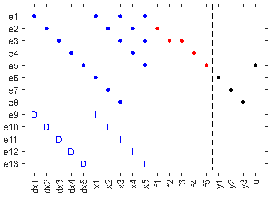
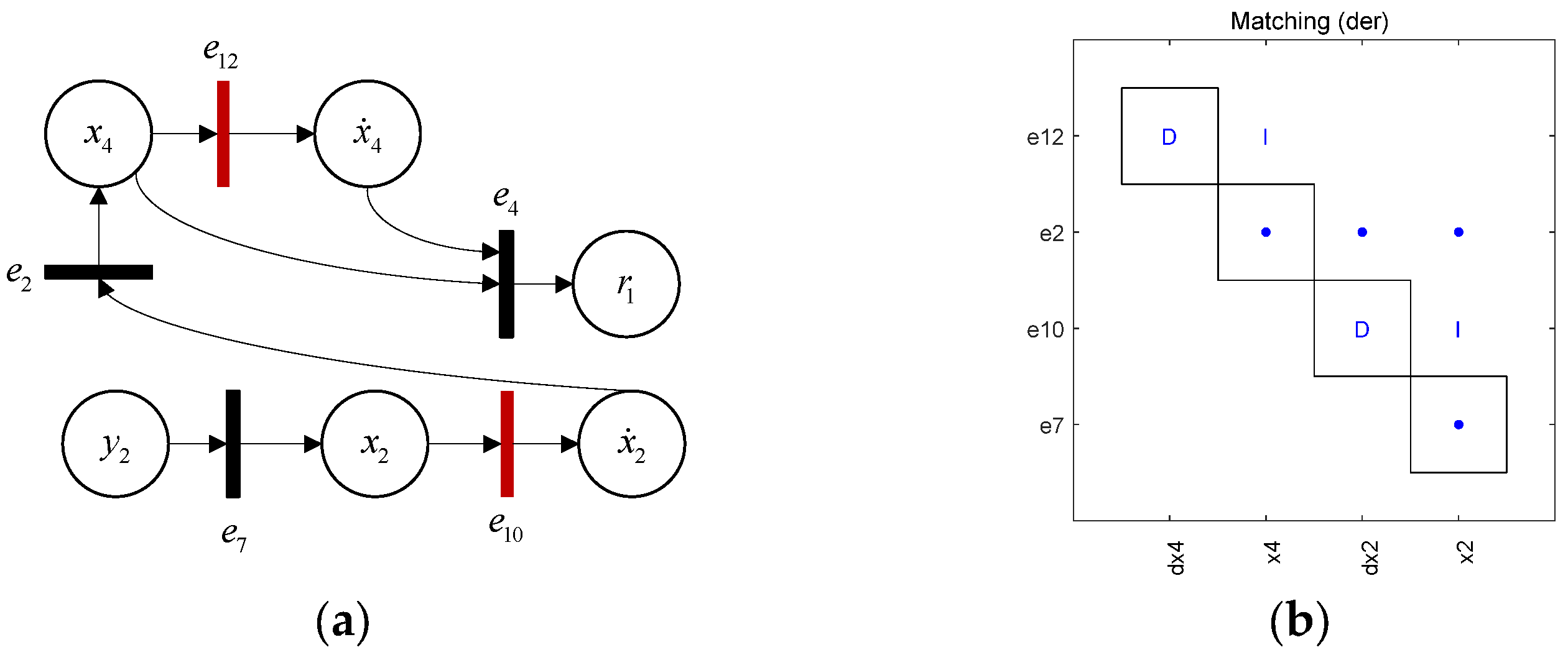
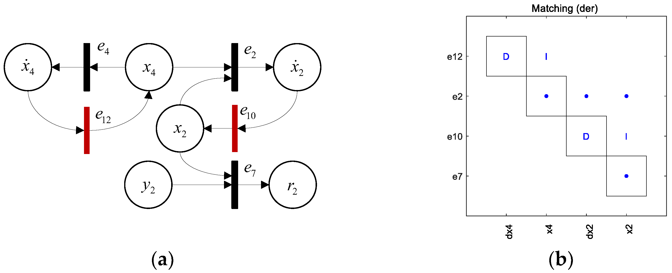
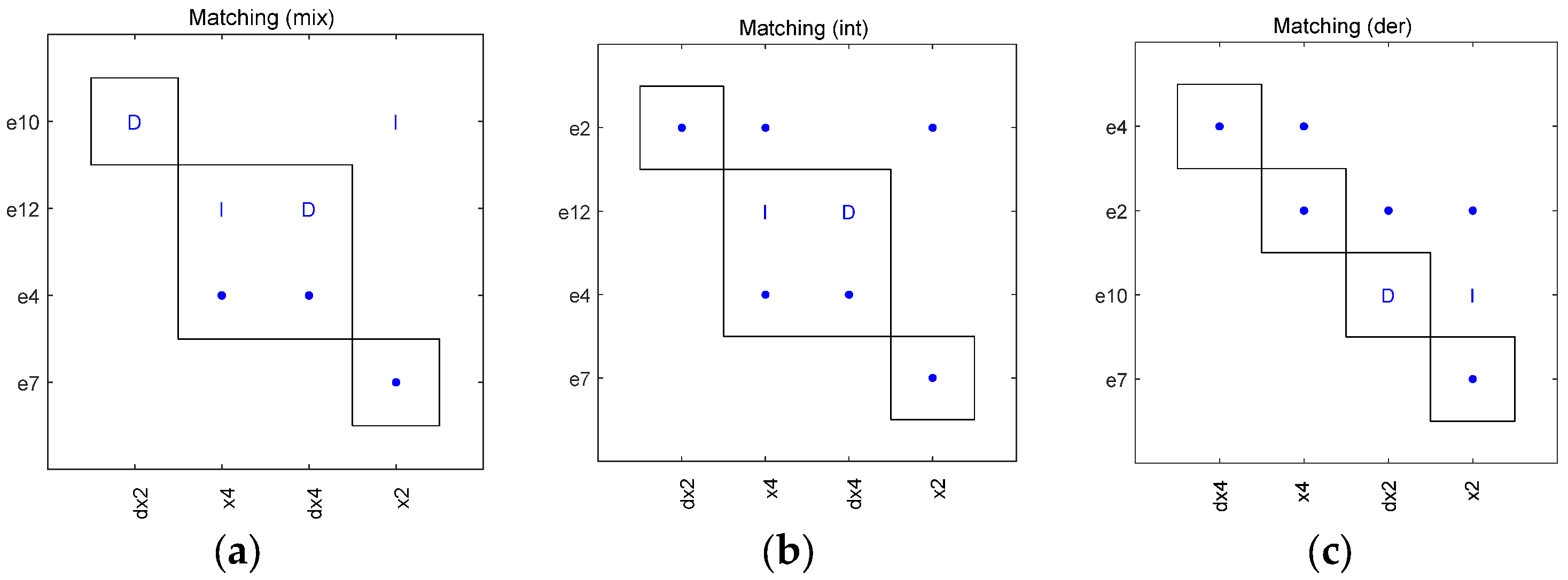
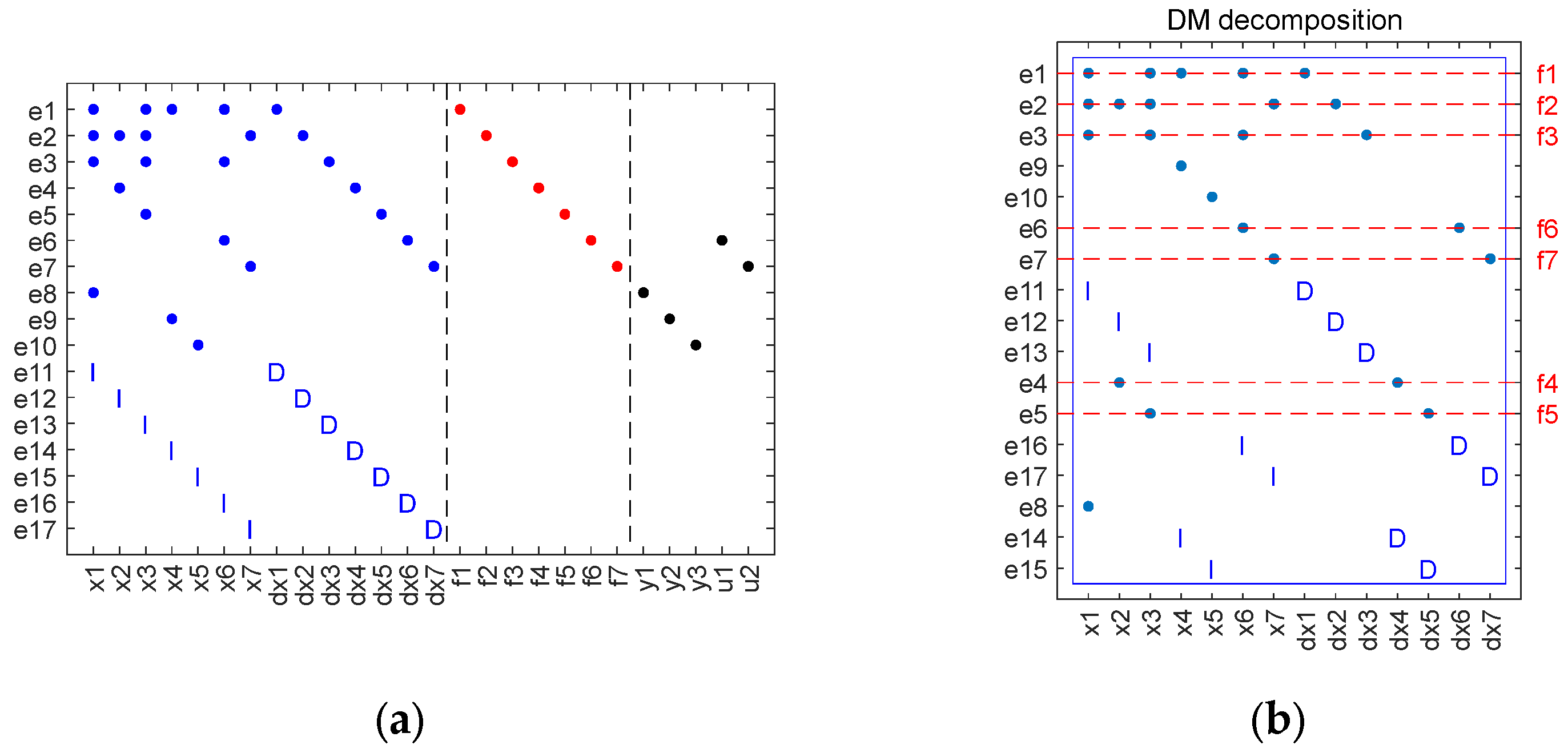
2.1.1. Structural Model

With its collection of variables $V$, set of constraint equations $E$, and edges $\overline{A}$, the structure of a system $M$ may be expressed as a graph $G\left(E,V,\overline{A}\right)$. If variable $v_j$ appears in equation $e_i$, it means that an edge $\left(e_i,v_j\right)$ exists between node $e_i$ and node $v_j$ of $G\left(E,V,\overline{A}\right)$. The set of edges can be denoted as $\overline{A}=\left\{\left(e_i,v_j\right)|e_i\in E,v_j\in V,v_j is in{e}_i\right\}$. For ease of presentation, $G\left(E,V,\overline{A}\right)$ can also be represented by its correlation matrix $A$, where $A\left(i,j\right)=1$ if an edge $\left(e_i,v_j\right)$ exists between nodes $e_i$ and $v_j$, and $A\left(i,j\right)=0$ otherwise.

The mathematical model of the system $M_1$ is expressed as:

$$\begin{array}{ll}{e}_1:{\dot{x}}_1=-2x_1+x_3+x_5\hfill & e_5:{\dot{x}}_5=-5x_5+u+f_5\hfill \\ e_2:{\dot{x}}_2=-3x_2+x_4+f_1\hfill & e_6:y_1=x_1\hfill \\ e_3:{\dot{x}}_3=-x_3+x_5+f_2+f_3\hfill & e_7:y_2=x_2\hfill \\ e_4:{\dot{x}}_4=-4x_4+f_4\hfill & e_8:y_3=x_3\hfill \end{array}$$

(1)

where ${\mathit{X}}_1=\left\{x_i,{\dot{x}}_i\right\}$ are the unknown state variables, $F_1=\left\{f_1,f_2,f_3,f_4\right\}$ are the system faults, and ${\mathit{Z}}_1=\left\{u,y_1,y_2,y_3\right\}$ are the known variables. To distinguish between ${\dot{x}}_i$ and $x_i$ in the structural model of $M_1$, the constraint equations are added here:

$$e_j:{\dot{x}}_i={\displaystyle \frac{d}{dt}}{x}_i,i=1,2,\dots ,5;j=9,10,\dots ,13$$

(2)

$G\left(E,V,\overline{A}\right)$ of $M_1$ is shown in Figure 2. In Figure 2, the variables are represented by the columns of the association matrix of $M_1$, and the rows indicate the equations. Among them, ‘•’ represents standard edges, ‘D’ represents edges related to ${\dot{x}}_i$ in the added constraint equations, and ‘I’ represents edges related to $x_i$ in the added constraint equations. The structural analysis exclusively focuses on the structure associated with the unknown variable $\mathit{X}$, i.e., the blue part in Figure 1. For ease of description, the structural model associated with $X$ is defined here as $G\left(E,X,\overline{A}\right)$.

2.1.2. Causal Diagnosability

The DM decomposition method [38] is frequently employed for structural analysis. The association matrix $A$ is divided into an upper triangular form by the DM decomposition, as shown in Figure 3a. The shaded elements in Figure 3a contain ‘0’ and ‘1’, and the blanks contain only ‘0’. The light-colored dashed line in the figure represents the maximum matching [27]. Matching refers to a set of edge sets that are not in the same row and column in the structural model. $M$ is divided into three parts after DM decomposition: the structurally underdetermined part $M^{-}=\left(E^{-},X^{-}\right)$, where $\left|E^{-}\right|<\left|X^{-}\right|$; the structurally exactly determined part $M^0=\left(E^0,X^0\right)$, where $\left|E^0\right|=\left|X^0\right|$; and the structurally overdetermined part $M^{+}=\left(E^{+},X^{+}\right)$, where $\left|E^{+}\right|>\left|X^{+}\right|$. A set of Hall components $\left\{G_i\right\}$ exist in $M^0$. Due to the resolved redundancy relations embedded in it [12], $M^{+}$ is the key to the structural analysis and the diagnostic focus. The DM decomposition of $M_1$ is shown schematically in Figure 3b, demonstrating that $M_1={\left(M_1\right)}^{+}$. Here, ${\left(\cdot \right)}^{+}$ and ${\left(\cdot \right)}^0$ are defined as the operators that obtain the structurally overdetermined and structurally exactly determined subsystems, respectively.

$E$ is said to be properly structurally overdetermined (SO) if $\left|E\right|>\left|Q_X\left(E\right)\right|$, where $Q_X\left(E\right)$ represents the unknown variables embedded in $E$. If $E$ is SO, this implies that a structurally overdetermined portion is present in the DM decomposition. Further, if $E=E^{+}$, it implies that $E$ is properly structurally overdetermined (PSO). If $E=E^{+}$, for $\forall e\in E$, $\exists E\backslash \left\{e\right\}$, $s.t.\left(E\backslash \left\{e\right\}\right)={\left(E\backslash \left\{e\right\}\right)}^{+}$. This states that a subset of the proper structurally overdetermined set $E$, PSO, exists. Furthermore, $E$ is said to be an MSO if $E$ is SO and there is no $\exists E^{\prime }\subseteq E$, such that $E^{\prime }$ is SO. The structural redundancy of MSO is 1, which is a minimal unit for diagnosability. Using the MSO method shown in the literature [39], the MSOs of $M_1$ can be obtained as $MS{O}_1=\left\{e_3,e_5,e_8,e_{11},e_{13}\right\}$, $MS{O}_2=\left\{e_2,e_4,e_7,e_{10},e_{12}\right\}$, $MS{O}_3=\left\{e_1,e_5,e_6,e_8,e_9,e_{13}\right\}$, $MS{O}_4=\left\{e_1,e_3,e_6,e_8,e_9,e_{11}\right\}$, $MS{O}_5=\left\{e_1,e_3,e_5,e_6,\right.\left.e_9,e_{11},e_{13}\right\}$.

Based on the MSO, the residuals are designed using the sequential residual method to analyze diagnosis. Taking $MS{O}_2$ as an example, residuals $r_1$ and $r_2$ are designed using $e_4$ and $e_7$ as redundant equations, respectively. Figure 4a and Figure 5a show the computation flow of $r_1$ and $r_2$, where the circles represent variables, the bars represent constraint equations, the red bars represent dynamic equations, and the arrows represent the computation flow. As shown in Figure 4a, the calculation process of $r_1$ is as follows: first, use $e_7$ to solve for the unknown variable $x_2$; then use $e_{10}$ to solve for ${\dot{x}}_2$; then use $e_2$ to solve for $x_4$; then use $e_{12}$ to solve for ${\dot{x}}_4$; and finally use $e_4$ to obtain $r_1$.

$$r_1:={\ddot{y}}_2+7{\dot{y}}_2+12y_2-{\dot{f}}_1-4f_1-f_4$$

(3)

Figure 4b shows the structural model of $MS{O}_2\backslash \left\{e_4\right\}$, and it can be seen that $MS{O}_2\backslash \left\{e_4\right\}=$${\left(MS{O}_2\backslash \left\{e_4\right\}\right)}^0$. The Hall component in the black border in Figure 4b is its maximum matching, i.e., $\left\{\left(e_7,x_2\right),\left(e_{10},{\dot{x}}_2\right),\left(e_2,x_4\right),\left(e_{12},{\dot{x}}_4\right)\right\}$. Comparing the two panels in Figure 4, it is observed that the process of solving for the unknown variables in Figure 4a is consistent with the matching process shown in Figure 4b. The matching variables are the solution variables of the matching equations. Because the matching contains only the differential edge ‘D’, $r_1$ is differentially causal. Causality here refers to integral and differential operations between dynamic variables. When no fault occurs, $r_1=0$. As $f_1$ appears in $e_2$ and $f_4$ appears in $e_4$, $r_1\ne 0$ when either $f_1$ or $f_4$ occurs. For ease of description, let ‘int’ denote integral causality, ‘der’ denote differential causality, and ‘mix’ denote mixed causality.

In the computational flow of $r_2$ shown in Figure 5a, two differential loops appear. One is the differential loop $\left(e_4,e_{12}\right)$ consisting of $e_4$ and $e_{12}$, and the other is the differential loop $\left(e_2,e_{10}\right)$ consisting of $e_2$ and $e_{10}$. Integral operations can break the differential loop. First, based on the differential loop $\left(e_4,e_{12}\right)$, one obtains $x_4={\displaystyle \frac{f_4}{4}}\left(1-e^{-4x_4}\right)+C{e}^{-4x_4}$ such that $x_4=h\left(f_4\right)$. Second, based on the differential loop $\left(e_2,e_{10}\right)$, one obtains $x_2={\displaystyle \frac{f_1+h\left(f_4\right)}{3}}\left(1-e^{-3x_2}\right)+C_1{e}^{-3x_2}$ such that $x_2=h\left(f_1,f_4\right)$. Finally, based on the redundant equation $e_7$, one obtains $r_2$, which is expressed as follows:

$$r_2=h\left(f_1,f_4\right)-y_2$$

(4)

Figure 5b shows the corresponding structural model of $MS{O}_2\backslash \left\{e_7\right\}$, which is structurally exactly determined. The Hall components of $MS{O}_2\backslash \left\{e_7\right\}$ are $G_1=\left\{\left(e_{12},x_4\right),\left(e_{12},d{x}_4\right),\right.\left.\left(e_4,x_4\right),\left(e_4,d{x}_4\right)\right\}$ and $G_2=\left\{\left(e_{10},x_2\right),\left(e_{10},d{x}_2\right),\left(e_2,x_2\right),\left(e_2,d{x}_2\right)\right\}$. Because $\left|G_1\right|>1$ and $\left|G_2\right|>1$, differential loops exist for $G_1$ and $G_2$. Since differential loops can only be broken by integral operations, $r_2$ is integrally causal. Because $r_2$ and $r_1$ involve the same constraint equations, the sensitivity of $r_2$ to faults is the same as that of $r_1$.

For $MS{O}_2$, when $e_2$, $e_{10}$, and $e_{12}$ are sequentially selected as the redundant equations, the causal matching relationship is shown in Figure 6. As shown in the figure, when $e_2$ is a redundant equation, $MS{O}_2$ is mixed causal. When $e_{10}$ is a redundant equation, $MS{O}_2$ is integrally causal. When $e_{12}$ is a redundant equation, $MS{O}_2$ is differentially causal. Therefore, the causality of MSO is related to its maximum matching. In addition to the matching edge ‘•’, if its maximal matching exists only in the differential edge ‘D’, it is differentially causal. If its maximal matching exists only in the integral edge ‘I’, it is integrally causal. If its maximal matching contains both integral and differential edges or only the standard edge ‘•’, then it is mixed causal. Equations (3) and (4) demonstrate that the duplicate MSO has the same sensitivity relation to faults, although its causal relations are different.

Therefore, the fault $f$ is said to be structurally detectable if and only if

$$\exists MSO, s.t. e_f\in MSO$$

(5)

where $e_f$ is the equation affected by $f$. For example, for $M_1$, $e_{f_1}=e_2$ and $e_{f_2}=e_{f_3}=e_3$. Further, the faults $f_i$ and $f_j$ are said to be structurally isolable if and only if

$$\exists MSO, s.t. e_{f_i}\in MSO\wedge e_{f_j}\notin MSO$$

(6)

The $MSOs=\left\{MS{O}_1,MS{O}_2,\dots ,MS{O}_s\right\}$ is known, and the set of faults is $F=\left\{f_1,f_2,\dots ,f_g\right\}$. The fault signature matrix (FSM) $FSM={\left[f{m}_{ij}\right]}_{g\times s}$ is built based on Equation (5) as follows:

$$f{m}_{ij}=\left\{\begin{array}{l}1, if e_{f_i}\in MC{R}_j\hfill \\ 0, otherwise\hfill \end{array}\right.$$

(7)

The fault isolation matrix (FIM) $FIM={\left[f_{ij}\right]}_{g\times g}$ is built based on Equation (6) as follows:

$$f_{ij}=\left\{\begin{array}{l}0, if \exists MC{R}_k, s.t. e_{f_i}\in MC{R}_k\wedge e_{f_j}\notin MC{R}_k\hfill \\ 1, otherwise\hfill \end{array}\right.$$

(8)

Based on the FSM, the fault detection rate (FDR) can be obtained as follows:

$$FDR={\displaystyle \frac{{\displaystyle \sum _{i=1}^{g}or\left(f{m}_{i\cdot }\right)}}{g}}$$

(9)

where $or\left(f{m}_{i\cdot }\right)$ refers to the logical or operation between the i-th row of data in the FSM. Based on FIM, the fault isolation rate (FIR) can be obtained as follows:

$$FIR=1-{\displaystyle \frac{{\displaystyle \sum _{i=1}^g{\displaystyle \sum _{j=1.i\ne j}^g{f}_{ij}}}}{g\left(g-1\right)}}$$

(10)

Taking $M_1$ as an example, the MSOs in which integral causality is implied are $\left\{MS{O}_1,MS{O}_2,MS{O}_3,MS{O}_5\right\}$, and their FSM and FIM are shown in Figure 7a and Figure 8a. Based on Equations (9) and (10), the FDR of $M_1$ under the integral causality condition is $FD{R}_1=100\%$, and the FIR is $FI{R}_1=70\%$. The MSOs of $M_1$, which imply differential causality, are $\left\{MS{O}_1,MS{O}_2,MS{O}_3,MS{O}_4\right\}$, and their FSM and FIM are shown in Figure 7b and Figure 8b. Based on Equations (9) and (10), it can be seen that the FDR under differential causality condition is $FD{R}_2=100\%$ and $FI{R}_2=80\%$. The MSOs in $M_1$ that imply mixed causality are $\left\{MS{O}_1,MS{O}_2,MS{O}_3,MS{O}_4,MS{O}_5\right\}$, and the FSM under mixed causality is shown in Figure 7c, in which $FD{R}_3=100\%$. The FIM under mixed causality is shown in 8c, where $FI{R}_3=80\%$. Here, the FDR is consistent under any causal constraints. The diagnosability results of mixed causality and differential causality are consistent, but the number of MSOs under different causal constraints is inconsistent.

2.2. Quantitative Assessment of Diagnosability Based on MMCD

The structural analysis method can only qualitatively analyze the diagnosability. Thus, this paper proposes a quantitative assessment method based on MMCD by fusing the advantages of MMD and MCD. MMCD not only compensates for the defects of MMD in measuring the covariance differences but also ensures the symmetry of the distance metric.

2.2.1. MMCD

MMD and MCD are both metrics formulated within a reproducible Hilbert space $\mathscr{H}$. MMD quantitatively describes the distance between probability distributions by calculating the mean difference in Hilbert space.

Definition 1 (MMD).

It is known that random variables $x$ and $y$ on the inner volume space $X$ obey probability distributions $p$ and $q$, respectively. Thus, the MMD between $x$ and $y$ is expressed as follows:

$$\begin{array}{cc}MMD\left[p,q,\mathscr{H}\right]& =\underset{h\in H}{\sup }\left|E_x\left[h\left(x\right)\right]-E_y\left[h\left(y\right)\right]\right|\\ & ={‖\mu \left[p\right]-\mu \left[q\right]‖}_{\mathscr{H}}\\ & =\sqrt{tr\left(KM\right)}\end{array}$$

(11)

where

$$K=\left[\begin{array}{cc}{K}_{XX}& K_{XY}\\ K_{YX}& K_{YY}\end{array}\right]$$

(12)

$$M_{ij}=\left\{\begin{array}{l}{\displaystyle \frac{1}{n^2}},\hspace{1em}{x}_i,x_j\in X\hfill \\ {\displaystyle \frac{1}{m^2}},\hspace{1em}{x}_i,x_j\in Y\hfill \\ -{\displaystyle \frac{1}{mn}},\hspace{1em}otherise\hfill \end{array}\right.$$

(13)

In addition, $E_x$ and $E_y$ denote the expectations of $x$ and $y$ , respectively; $H$ is the fundamental function $h:X\mapsto ℝ$ of $\mathscr{H}$; $\mu \left[p\right]$ and $\mu \left[q\right]$ represent the mean map of $p$ and $q$ on $\mathscr{H}$, respectively; ${\left(K_{XX}\right)}_{ij}=k\left(x_i,x_j\right)$, ${\left(K_{XY}\right)}_{ij}=k\left(x_i,y_j\right)$, ${\left(K_{YY}\right)}_{ij}=k\left(y_i,y_j\right)$ , and $k\left(x,y\right)$ are regenerated kernels of $\mathscr{H}$.

Through calculating the maximum covariance difference in Hilbert space, MCD provides a quantitative representation of the separation between probability distributions.

Definition 2 (MCD).

It is known that random variables $x$ and $y$ on the inner volume space $X$ obey probability distributions $p$ and $q$ , respectively. Thus, the MCD between $x$ and $y$ is expressed as follows:

$$\begin{array}{cc}MCD\left[p,q,\mathscr{H}\right]& =\underset{‖a‖\le 1}{\sup }{\displaystyle \sum _{i,j\in I}{a}_{ij}\left(\mathrm{cov}\left[e_i\left(x\right),e_j\left(x\right)\right]\right)-\mathrm{cov}\left[e_i\left(y\right),e_j\left(y\right)\right]}\\ & ={‖C\left[p\right]-C\left[q\right]‖}_{HS}\\ & =\sqrt{tr\left(KZKZ\right)}\end{array}$$

(14)

where

$$\mathrm{cov}\left[e_i\left(x\right),e_j\left(x\right)\right]=E_x\left[e_i\left(x\right),e_j\left(x\right)\right]-E_x\left[e_i\left(x\right)\right]E_x\left[e_j\left(x\right)\right]$$

(15)

$$Z_{ij}=\left\{\begin{array}{l}{\displaystyle \frac{1}{n}}-{\displaystyle \frac{1}{n^2}},\hspace{1em}i=j,x_i\in X\hfill \\ -{\displaystyle \frac{1}{n^2}},\hspace{1em}i\ne j,x_i\in X,x_j\in X\hfill \\ {\displaystyle \frac{1}{m^2}}-{\displaystyle \frac{1}{m}},\hspace{1em}i=j,x_i\in Y\hfill \\ \begin{array}{l}{\displaystyle \frac{1}{m^2}},\hspace{1em}\hspace{1em}i\ne j,x_i\in Y,x_j\in Y\hfill \\ 0,\hspace{1em}otherwise\hfill \end{array}\hfill \end{array}\right.$$

(16)

In addition, $‖a‖={\left({\displaystyle {\sum }_{i,j\in I}{a}_{ij}^2}\right)}^{1/2}$; $e_i$ is the orthonormal basis of $\mathscr{H}$; $C\left[p\right]$ is the covariance operator on $\mathscr{H}$; ${‖\cdot ‖}_{HS}$ is the Hilbert–Schmidt (HS) paradigm; and $\mathit{X}=\left\{x_1,\dots ,x_n\right\}$ and $\mathit{Y}=\left\{y_1,\dots ,y_m\right\}$ are the finite number of observations sampled sequentially from distributions $p$ and $q$ , respectively.

Through combining the differences between MCD and MMD in Hilbert space, MMCD provides a quantitative description of the distance between probability distributions.

Definition 3 (MMCD).

It is known that random variables  $x$ and $y$ on the inner volume space $\mathit{X}$ obey probability distributions $p$ and $q$ , respectively. Thus, the MMCD between $x$ and $y$ is expressed as follows:

$$\begin{array}{c}MMCD\left[p,q,\mathscr{H}\right]={\left({‖\mu \left[p\right]-\mu \left[q\right]‖}_{\mathscr{H}}^2+\beta {‖C\left[p\right]-C\left[q\right]‖}_{HS}^2\right)}^{1/2}\\ =\sqrt{tr\left(KM\right)+\beta tr\left(KZKZ\right)}\end{array}$$

(17)

where $\beta \in \left[0,1\right]$.

Comparison of Equations (11), (14), and (17) shows that MMCD can take into account the mean difference and covariance difference of the probability distribution. Analyzing numerically, we find that $MMCD\left[p,q,\mathscr{H}\right]>MMD\left[p,q,\mathscr{H}\right]$ and $MMCD\left[p,q,\mathscr{H}\right]>MCD\left[p,q,\mathscr{H}\right]$. Therefore, the MMCD can measure the probability distribution differences more fully. As $MMCD\left[p,q,\mathscr{H}\right]=MMCD\left[q,p,\mathscr{H}\right]$, the MMCD also satisfies the symmetry constraint.

2.2.2. Quantitative Assessment

The sensitivity that exists between MSO and faults may be transformed into a leapfrog connection between residuals and faults using MSO design residuals. When there is no fault, the noise affects $r$, and the probability distribution of $r$ and the noise are identical. When a fault occurs, $r$ is affected by the fault, and the distribution of $r$ is different. Subject to causality constraints, the distribution of $r$ is also different for causal relationships. Here, a quantitative assessment technique based on MMCD is suggested to gauge how sensitive residuals are to faults. Based on $MSOs=\left\{MS{O}_1,MS{O}_2,\dots ,MS{O}_s\right\}$, the residuals $R=\left\{r_1,r_2,\dots ,r_s\right\}$ are designed. The faults are known to be $F=\left\{f_1,f_2,\dots ,f_g\right\}$, such that $NF$ represents the no-fault mode. Assume that the probability distribution of $R$ is $p_{NF}$ when no fault occurs, which is denoted as $R\sim p_{NF}$, and the probability distribution of $R$ is $p_{f_i}$ when the fault $f_i$ occurs, which is denoted as $R\sim p_{f_i}$. Relying on MMCD, the detection complexity $D\left(f_i,NF\right)$ of $f_i$ is expressed as follows:

$$D\left(f_i,NF\right)=MMCD\left(p_{f_i},p_{NF},\mathscr{H}\right)$$

(18)

The isolation complexity $D\left(f_i,f_j\right)$ for $f_i$ and $f_j$ is expressed as follows:

$$D\left(f_i,f_j\right)=MMCD\left(p_{f_i},p_{f_j},\mathscr{H}\right)$$

(19)

Due to uncertainties such as noise and interference, $D\left(f_i,NF\right)>0$ cannot be used to determine whether $f_i$ occurs, and $D\left(f_i,f_j\right)>0$ cannot determine whether $f_i$ and $f_j$ can be isolated. Thus, it is essential to establish the detectability limit ${\sigma }_D$ and isolability limit ${\sigma }_I$ to judge the diagnosability. In NF, the residual $R_1$ and $R_2$ of multiple repeated experiments are taken, and their probability distributions are $p_{NF}$ and $q_{NF}$, respectively. The diagnosability limit is expressed as follows:

$${\sigma }_D=\underset{i}{\max }\left\{MMCD\left(p_{NF},0,\mathscr{H}\right)\right\}$$

(20)

$${\sigma }_I=\underset{i}{\max }\left\{MMCD\left(p_{NF},q_{NF},\mathscr{H}\right)\right\}$$

(21)

where $\underset{i}{\max }$ indicates the maximum value taken from several experiments. Therefore, if $D\left(f_i,NF\right)>{\sigma }_D$, it means that $f_i$ can be detected, and the larger $\left|D\left(f_i,NF\right)-{\sigma }_D\right|$ is, the more straightforward it is to detect $f_i$. If $D\left(f_i,f_j\right)>{\sigma }_I$, it means that the $f_i$ can be isolated from $f_j$, and the larger $\left|D\left(f_i,f_j\right)-{\sigma }_I\right|$ is, the lower the isolation difficulty of $f_i$ and $f_j$.

Based on Equation (19), a quantitative assessment matrix $D$ is established:

$$D=\left[\begin{array}{ccccc}D\left(f_1,NF\right)& D\left(f_1,f_1\right)& D\left(f_1,f_2\right)& \dots & D\left(f_1,f_g\right)\\ D\left(f_2,NF\right)& D\left(f_2,f_1\right)& D\left(f_2,f_2\right)& \dots & D\left(f_2,f_g\right)\\ ⋮& ⋮& ⋮& \ddots & ⋮\\ D\left(f_g,NF\right)& D\left(f_g,f_1\right)& D\left(f_g,f_2\right)& \dots & D\left(f_g,f_g\right)\end{array}\right]$$

(22)

where $D\left(f_i,NF\right)$ indicates the detection complexity of the diagnostic system $R$ for $f_i$, and $D\left(f_i,f_j\right)$ indicates the isolation complexity of $R$ for $f_i$ and $f_j$, $i,j=1,2,\dots ,g$. Given that MMCD has symmetry, $D\left(f_i,f_j\right)=D\left(f_j,f_i\right)$. As a single fault itself does not need to be considered for isolation, $D\left(f_i,f_i\right)=0$. Based on Equations (20)~(22), the fault diagnosis matrix $D_d={\left[d_{ij}\right]}_{g\times \left(g+1\right)}$ is established.

$$d_{ij}=\left\{\begin{array}{l}1, if D\left(f_i,NF\right)>{\sigma }_D\wedge j=1\hfill \\ 1, if D\left(f_i,f_j\right)\le {\sigma }_I\vee D\left(f_i,f_i\right)=0\hfill \\ 0, otherwise\hfill \end{array}\right.$$

(23)

Based on $D_d$, the FDR is expressed as follows:

$$FDR={\displaystyle \frac{{\displaystyle \sum _{i=1}^g{d}_{i1}}}{g}}$$

(24)

The FIR is expressed as follows:

$$FIR=1-{\displaystyle \frac{{\displaystyle \sum _{i=1}^g{\displaystyle \sum _{j=2,i\ne j}^{g+1}{d}_{ij}}}}{g\left(g-1\right)}}$$

(25)

2.3. Diagnosability Optimization Design Using GWO Algorithm

2.3.1. Optimization Design Model

The number of MSOs grows exponentially with increasing redundancy in the system structure. Thus, to save design costs while designing the diagnostic system, it is necessary to optimize the optimal MSO from MSOs for diagnostic system design. Taking the causality constraints and diagnostic requirements into account, the steps of the diagnostic optimal design model are as follows:

• Step 1: Build the system structure model $G\left(E,X,\overline{A}\right)$;
• Step 2: Using the causal MSO algorithm from the literature [27], obtain the $MSOs=\left\{MS{O}_1,MS{O}_2,\dots ,MS{O}_s\right\}$ under different causal conditions;
• Step 3: Design the residual set $R_{con}=\left\{r_1,r_2,\dots ,r_w\right\}$ that satisfies the diagnosability requirement;
• Step 4: Construct the vector $\mathit{c}={\left[c_i\right]}_{1\times w}$;

$$c_i=\left\{\begin{array}{l}1, if r_i is selected\hfill \\ 0, otherwise\hfill \end{array}\right.$$

(26)

Then, the optimized diagnostic system is $R:=R_{con}.\ast c$. Based on MMCD, a quantitative assessment matrix $D$ is established for $R$.

• Step 5: Assume that the design cost of $R_{con}$ is $\gamma ={\left[{\gamma }_i\right]}_{1\times w}$. Then, the design cost of $R$ is expressed as follows:

$$cost={\displaystyle \sum _{i=1}^w{\gamma }_i{c}_i}$$

(27)

In summary, the diagnostic optimization model can be expressed as follows:

$$min cost={\displaystyle \sum _{i=1}^b{\gamma }_i{c}_i}$$

(28)

$$s.t. D\ge D^{req}$$

(29)

where $D^{req}$ represents the quantitative demand matrix, typically the diagnosability limit $\sigma$.

2.3.2. Diagnosability Optimization Design Strategy Based on the GWO Algorithm

The GWO algorithm is a new type of pack intelligence optimization algorithm that mimics the hunting behavior and social hierarchy of gray wolf packs. Individual wolves are generally divided into four classes; namely, $\alpha$, $\beta$, $\delta$, and $\omega$ wolves. Among them, the $\alpha$ wolf is the leader, representing the optimal solution in the population, and is the supreme ruler and manager of the wolf pack. The $\beta$ and $\delta$ wolves represent the second- and third-best solutions in the population, and the remaining solutions are regarded as $\omega$ wolves.

The optimization process of the GWO algorithm is divided into three steps: first, searching and tracking the prey; second, hunting and encircling the prey until the prey stops moving; and finally, attacking the prey. The position update formula for the wolves searching and surrounding prey is expressed as follows:

$$\mathit{X}\left(t+1\right)={\mathit{X}}_p\left(t\right)-\mathit{A}\cdot \mathit{D}$$

(30)

where

$$\mathit{D}=\left|\mathit{C}\cdot {\mathit{X}}_p\left(t\right)-\mathit{X}\left(t\right)\right|$$

(31)

In the above equation, $t$ is the current iteration number, ${\mathit{X}}_p$ is the prey position, $\mathit{X}$ is the gray wolf position, and $\mathit{A}$ and $\mathit{C}$ are the coefficient vectors of the algorithm.

$$\mathit{A}=2\mathit{a}\cdot \mathit{r}\mathit{a}\mathit{n}{\mathit{d}}_1-\mathit{a}$$

(32)

$$\mathit{C}=2\mathit{r}\mathit{a}\mathit{n}{\mathit{d}}_2$$

(33)

Here, $\mathit{r}\mathit{a}\mathit{n}{\mathit{d}}_1$ and $\mathit{r}\mathit{a}\mathit{n}{\mathit{d}}_2$ are random vectors between $\left[0,1\right]$, and $\mathit{a}$ is the tuning parameter, which is expressed as follows:

$$a=2\left(1-{\displaystyle \frac{t}{t_{\max }}}\right)$$

(34)

where $t_{\max }$ is the maximum number of iterations and $\mathit{A}\in \left[-2\mathit{a},2\mathit{a}\right]$, $\mathit{C}\in \left[0,2\right]$.

The position of the $\omega$ wolf is based on the positions of $\alpha$ wolf, $\beta$ wolf, and $\delta$ wolf. Therefore, once the positions of $\alpha$ wolf, $\beta$ wolf, and $\delta$ wolf have been determined, the location of the prey can be determined based on the distance between them.

$$\left\{\begin{array}{l}{\mathit{X}}_{\alpha }\left(t+1\right)={\mathit{X}}_{\alpha }\left(t\right)-{\mathit{A}}_1\cdot \left|{\mathit{C}}_1\cdot {\mathit{X}}_{\alpha }\left(t\right)-\mathit{X}\left(t\right)\right|\hfill \\ {\mathit{X}}_{\beta }\left(t+1\right)={\mathit{X}}_{\beta }\left(t\right)-{\mathit{A}}_2\cdot \left|{\mathit{C}}_2\cdot {\mathit{X}}_{\beta }\left(t\right)-\mathit{X}\left(t\right)\right|\hfill \\ {\mathit{X}}_{\delta }\left(t+1\right)={\mathit{X}}_{\delta }\left(t\right)-{\mathit{A}}_3\cdot \left|{\mathit{C}}_3\cdot {\mathit{X}}_{\delta }\left(t\right)-\mathit{X}\left(t\right)\right|\hfill \\ {\mathit{X}}_{\omega }\left(t+1\right)={\displaystyle \sum _{j=\alpha ,\beta ,\delta }{w}_j{\mathit{X}}_j\left(t+1\right)}\hfill \end{array}\right.$$

(35)

Here, $w_j$ is the weighting factor for $\alpha$, $\beta$, and $\delta$ wolves.

$$w_j={\displaystyle \frac{f\left({\mathit{X}}_j\left(t\right)\right)}{f\left({\mathit{X}}_{\alpha }\left(t\right)\right)+f\left({\mathit{X}}_{\beta }\left(t\right)\right)+f\left({\mathit{X}}_{\delta }\left(t\right)\right)}}$$

(36)

In the above equation, $f\left({\mathit{X}}_j\left(t\right)\right)$ denotes the acclimatization value of the j-th gray wolf individual in the t-th generation.

The optimal design strategy for causal diagnosability based on the GWO algorithm is outlined below.

• Step 1: For parameter initialization, set the gray wolf population as $N=50$, maximum iteration number $t_{\max }=20$, and parameters $\mathit{a}$, $\mathit{A}$, and $\mathit{C}$. The parameters of MMCD are selected from the optimal parameter settings verified in the literature [40];
• Step 2: Based on Equation (26), initialize the position of the gray wolf population $\mathit{X}$;
• Step 3: If the constraints shown in Equation (29) are satisfied, calculate its fitness value based on Equation (28); otherwise, its fitness value is infinity. Second, determine the $\alpha$ wolf, $\beta$ wolf, and $\delta$ wolf according to the merit of fitness;
• Step 4: Update the location of the gray wolf population based on Equation (35);
• Step 5: Update the parameters $\mathit{a}$, $\mathit{A}$, and $\mathit{C}$;
• Step 6: Judge whether the maximum number of iterations has been reached. If so, stop the algorithm and return as the optimal solution ${\mathit{X}}_{\alpha }$; otherwise, return to step 3.

3. Results and Analysis

In this section, causal diagnosability is optimally designed based on the fixed-wing UAV structural model. Section 3.1 establishes the UAV structural model and analyzes its structural characteristics and its causal diagnosability. In Section 3.2, based on the MSO, the system residuals are designed, and the influencing factors of diagnosability are studied in a simulation scenario. In Section 3.3, based on the MMCD, the probability distribution difference of fault residuals is measured to evaluate quantitatively the system’s diagnosability. In Section 3.4, to minimize the cost of the diagnostic system design under the premise of maximizing the system’s diagnosability requirements, the optimal diagnostic system is optimized based on the GWO algorithm for the diagnosability of the UAV.

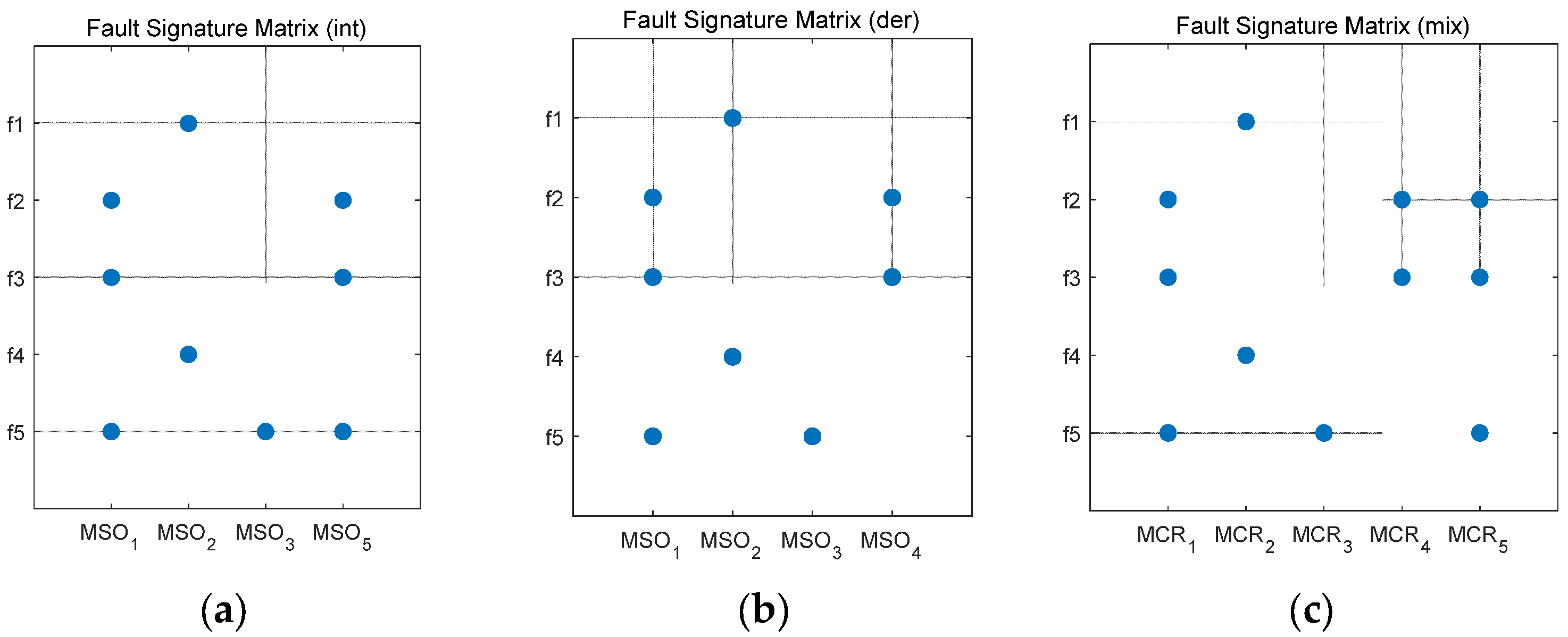
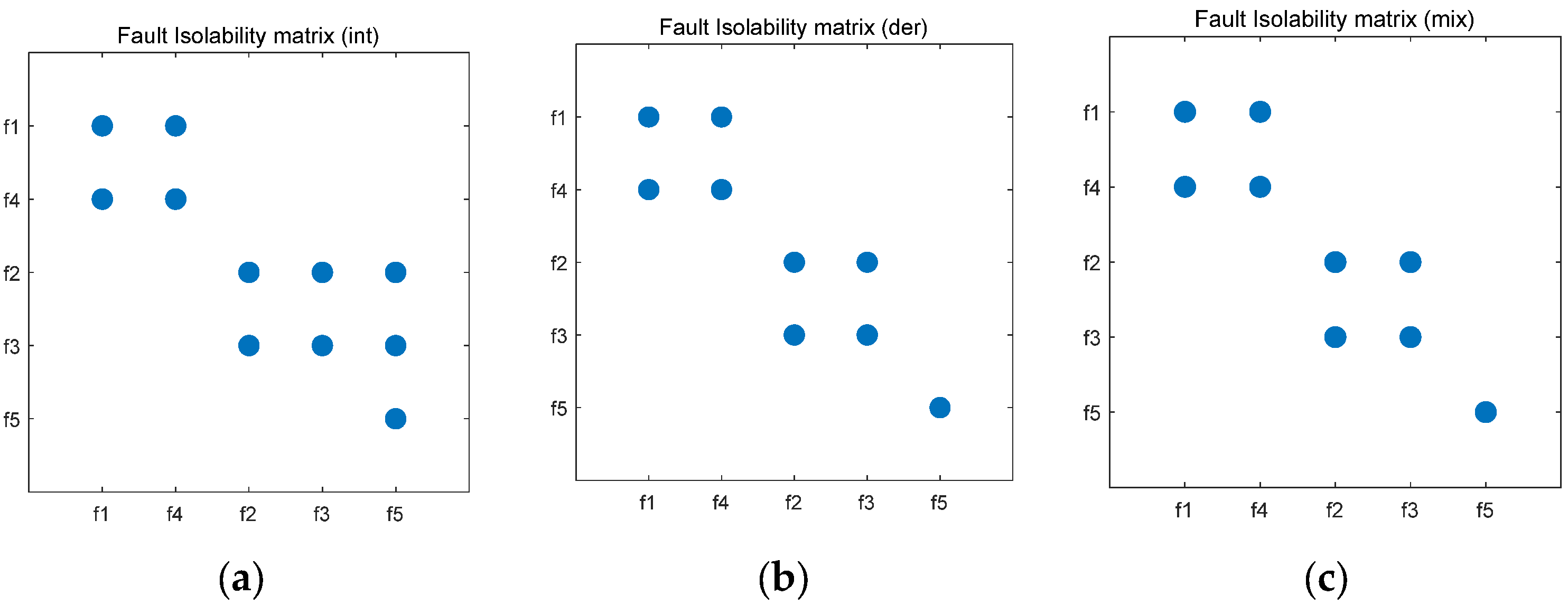
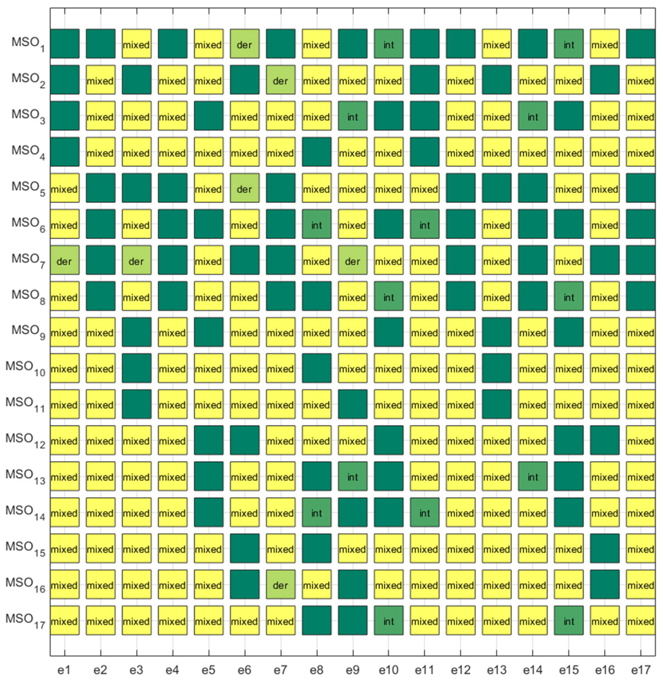
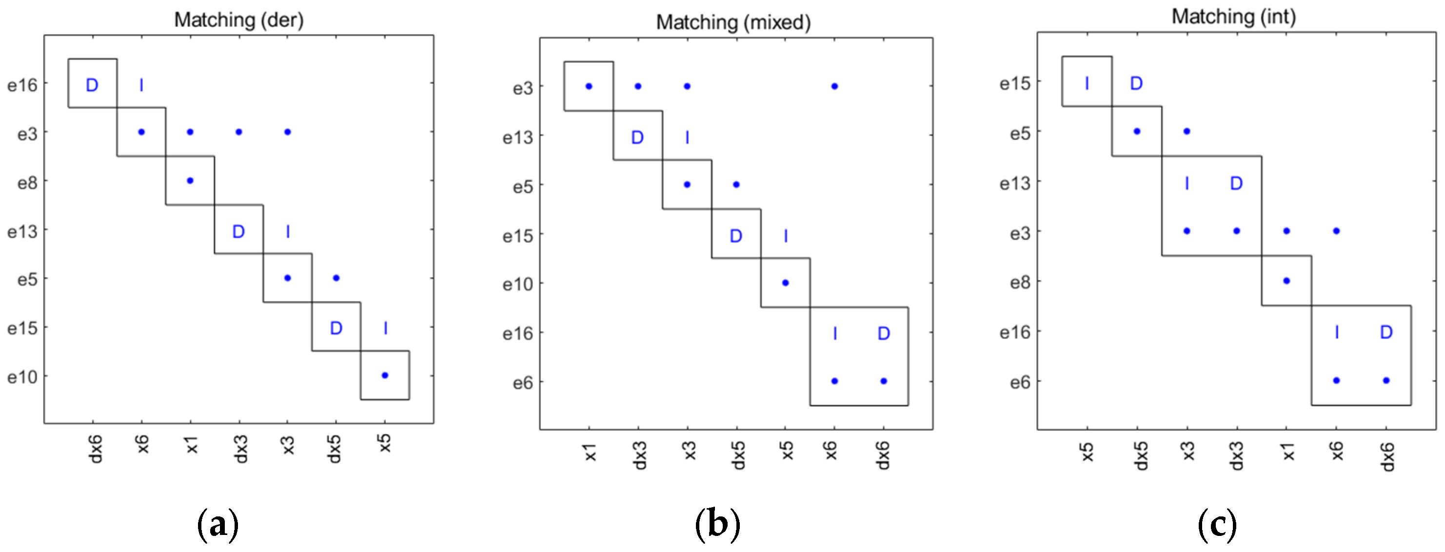
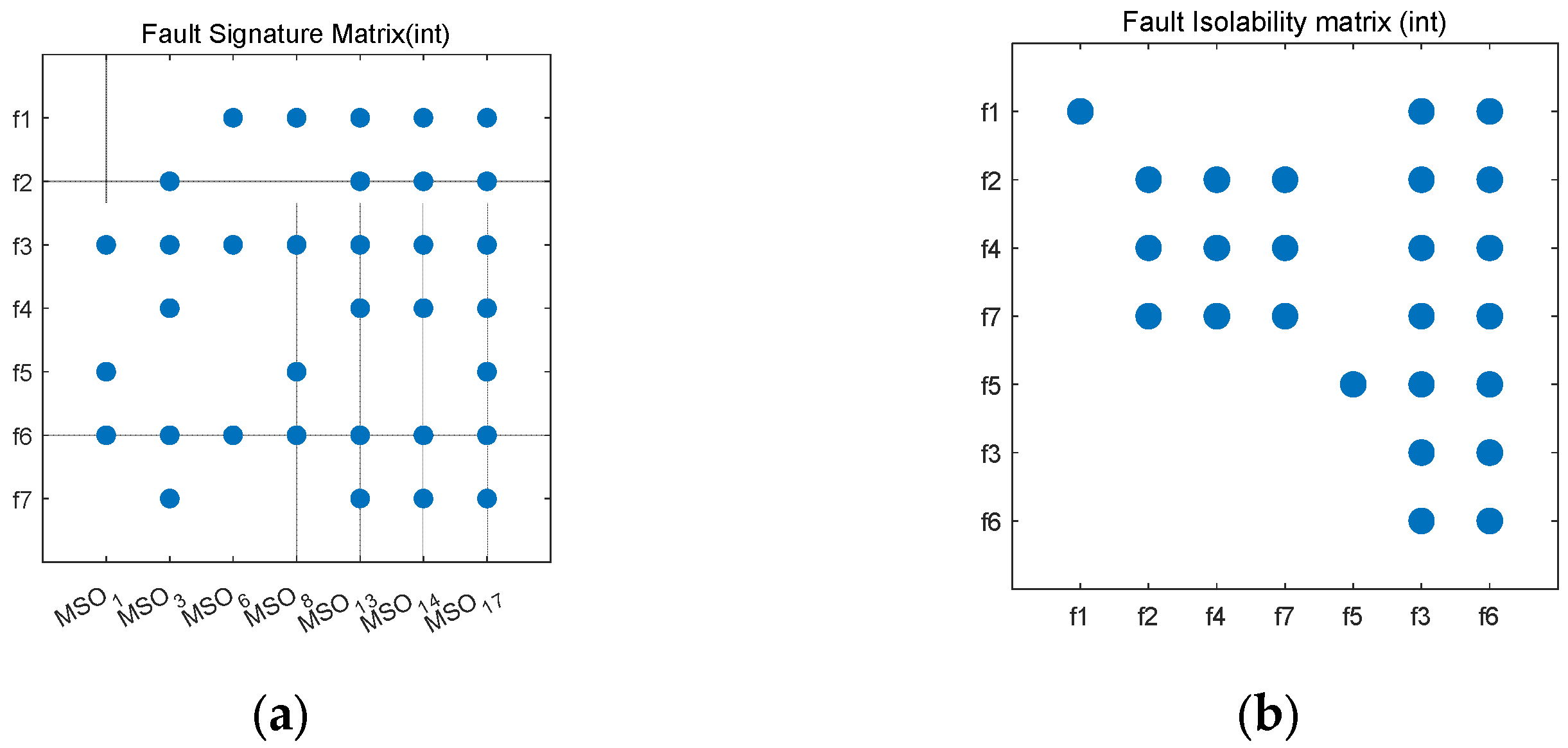
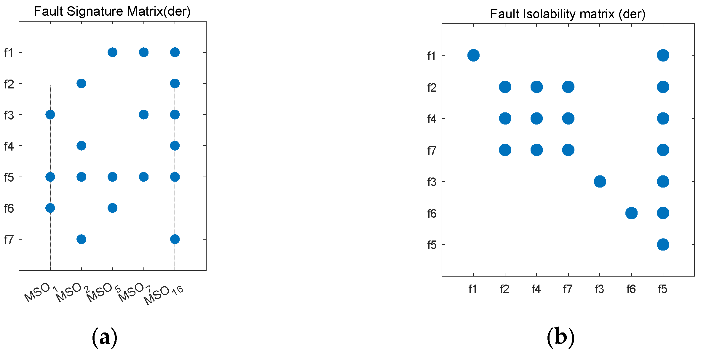
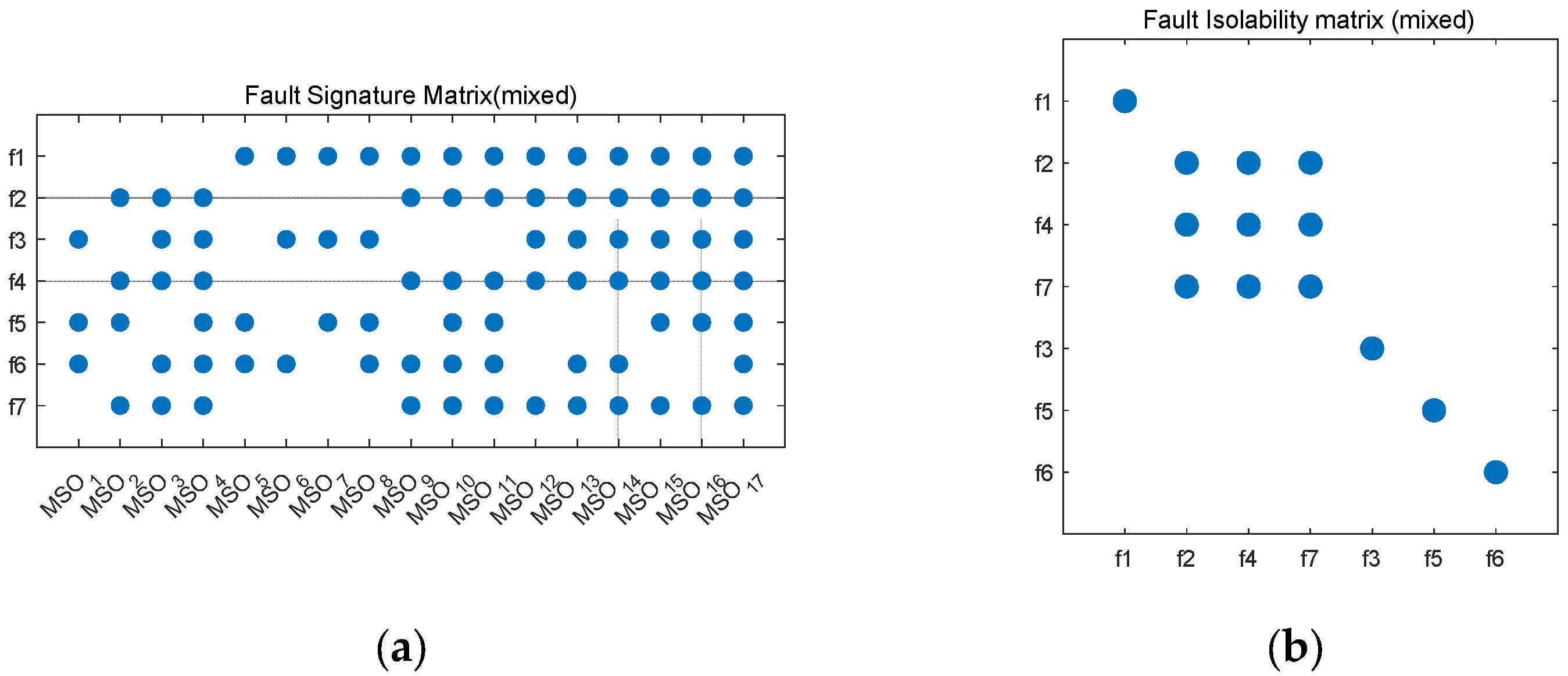
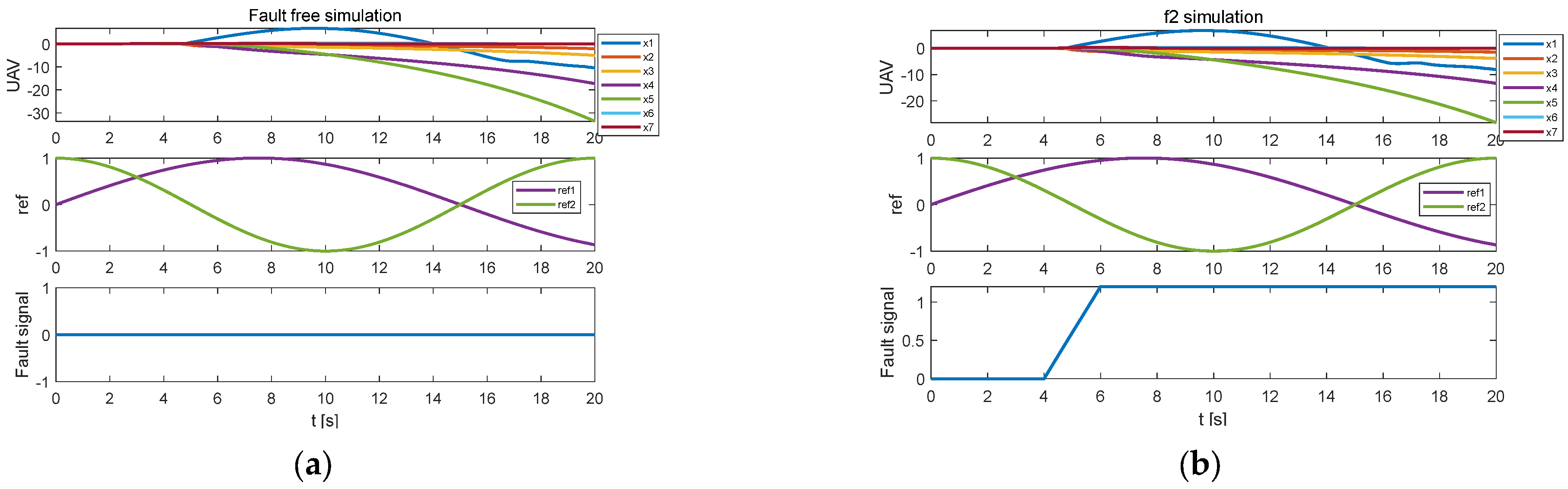
3.1. Causal Diagnosability of Fixed-Wing UAVs

For simulation verification in this research, the fixed-wing UAV model $M_{UAV}$ from the literature [27] is utilized, and the mathematical model is expressed as follows:

$$\begin{array}{l}\dot{\mathit{x}}=A\mathit{x}+B\mathit{u}+\mathit{F}\\ \mathit{y}=C\mathit{x}\end{array}$$

(37)

where $\mathit{x}={\left[x_1,x_2,\dots ,x_7\right]}^T$ are the system states, $\mathit{u}={\left[u_1,u_2\right]}^T$ are the system inputs, $\mathit{F}={\left[f_1,f_2,f_3,f_4,f_5,f_6,f_7\right]}^T$ are the system faults, and $\mathit{y}={\left[y_1,y_2,y_3\right]}^T$ are the system outputs.

$$A=\left[\begin{array}{ccccccc}-0.28& 0& -32.90& 9.81& 0& -5.43& 0\\ -0.10& -8.325& 3.75& 0& 0& 0& -28.64\\ 0.37& 0& -0.64& 0& 0& -9.49& 0\\ 0& 1& 0& 0& 0& 0& 0\\ 0& 0& 1& 0& 0& 0& 0\\ 0& 0& 0& 0& 0& -10& 0\\ 0& 0& 0& 0& 0& 0& -5\end{array}\right]$$

(38)

$$B={\left[\begin{array}{lllllll}0\hfill & 0\hfill & 0\hfill & 0\hfill & 0\hfill & 20\hfill & 0\hfill \\ 0\hfill & 0\hfill & 0\hfill & 0\hfill & 0\hfill & 0\hfill & 10\hfill \end{array}\right]}^T$$

(39)

$$C=\left[\begin{array}{ccccccc}1& 0& 0& 0& 0& 0& 0\\ 0& 0& 0& 1& 0& 0& 0\\ 0& 0& 0& 0& 1& 0& 0\end{array}\right]$$

(40)

The structural model of $M_{UAV}$ and the DM decomposition schematic are shown in Figure 9. As shown in Figure 9a, the dynamic constraint equation shown in Equation (2) is also added to the structural model of $M_{UAV}$. As shown in Figure 9b, $M_{UAV}={\left(M_{UAV}\right)}^{+}$.

Using the search method reported in the literature [27], the MSOs of $M_{UAV}$ can be obtained as shown in Figure 10. The rows of the matrix in Figure 10 illustrate the MSOs, the columns illustrate the equations, and the elements of the matrix contain {‘int’, ‘der’, ‘mixed’} as well as empty elements. The empty element of the matrix means that the equation corresponding to the column in which the position is located is not among the MSOs corresponding to its row. If the element of the matrix is not empty (i.e., {‘int’, ‘der’, ‘mixed’}), it means that the equation corresponding to the column where the position is located is in the MSO corresponding to the row. As an example, $MS{O}_1=\left\{e_3,e_5,e_6,e_8,e_{10},e_{13},e_{15},e_{16}\right\}$. Further, suppose the matrix element is ‘int’(‘der’, ‘mixed’). In this case, it means that when the equation corresponding to the column in which the position is located is selected as the redundant equation, MSO is integrally (differential, mixed) causal. Taking $MS{O}_1$ as an example, if $e_6$, $e_8$, and $e_{10}$ are selected as redundant equations, the causal relationships are shown in Figure 11. As shown in Figure 11a, when $e_6$ is chosen as the redundant equation, the maximum matching relation of $MS{O}_1$ contains only ‘D’ except for the normal edges, so it is differentially causal. Similarly, when $e_8$ is a redundant equation, $MS{O}_1$ is mixed causal; when $e_{10}$ is a redundant equation, $MS{O}_1$ is integrally causal.

Based on Figure 10, the integrally causal MSOs of $M_{UAV}$ are $intMSOs=\left\{MS{O}_1,MS{O}_3,MS{O}_6,MS{O}_8,MS{O}_{13},MS{O}_{14},MS{O}_{17}\right\}$. Based on Equations (7) and (8), the FSM and FIM of $intMSOs$ are established as shown in Figure 12. The dot in the figure represents matrix element 1. As shown in Figure 12a, under the integral causality condition, $FD{R}_4=100\%$. From Figure 12b, $FI{R}_4=57.14\%$. Based on Figure 10, the differential causal MSOs are $derMSOs=\left\{MS{O}_1,MS{O}_2,MS{O}_5,MS{O}_7,MS{O}_{16}\right\}$. The FSM and FIM of $derMSOs$ are shown in Figure 13, with $FD{R}_5=100\%$ and $FI{R}_5=71.43\%$. Based on Figure 10, the mixed causal MSOs can be obtained as $mixMSOs=\left\{MS{O}_1,MS{O}_2,\dots ,MS{O}_{17}\right\}$. The diagnosability result of $mixMSOs$ is shown in Figure 14, with $FD{R}_6=100\%$, and $FI{R}_6=85.71\%$. It can be found that the diagnosability is different under different causal constraints, with the best diagnosability obtained under mixed causal constraints and the worst diagnosability obtained under integral causal constraints. This further validates the effect of causality on diagnosability.

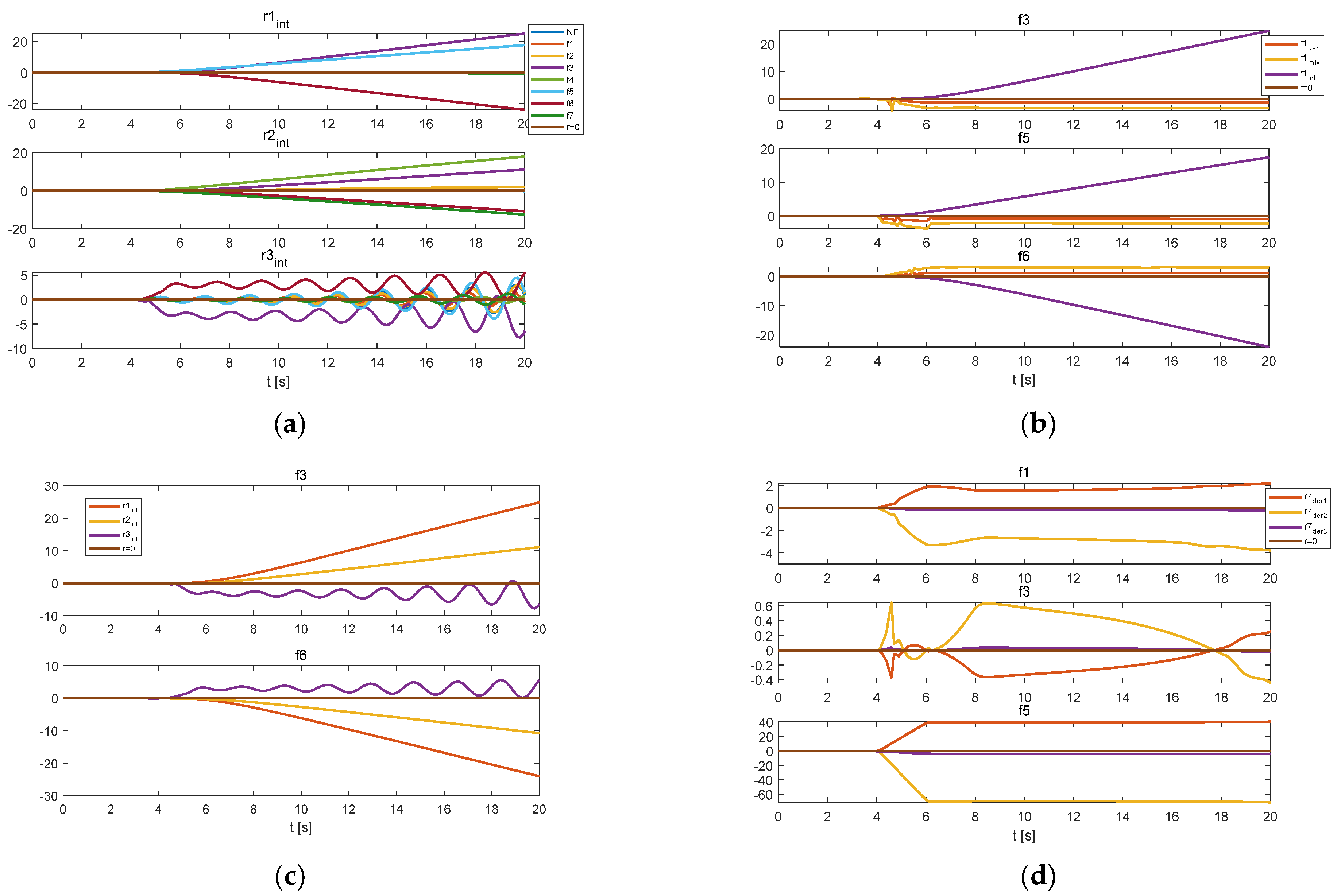
3.2. Diagnosability Impact Factor Analysis

To verify the diagnosability of different faults and the responsiveness linking MSOs to faults, the sequential residual method is used for residual design. Figure 15a displays the simulation results of $M_{UAV}$ without fault, where $re{f}_1$ and $re{f}_2$ are the reference input signals. When $f_2$ occurs, the simulation results of $M_{UAV}$ are shown in Figure 15b, and all the system faults are slope faults as shown in the figure. The used simulation software was MATLAB (2021b version). The initial state of the system is ${\mathit{x}}_0={\left[0\right]}_{1\times 7}^{\mathrm{T}}$, and noise is not considered here. Based on $MS{O}_1$ ($MS{O}_3$, $MS{O}_6$), $e_{10}$ ($e_9$, $e_8$) is selected as the redundancy equation to design the residual $r{1}_{\mathrm{int}}$ ($r{2}_{\mathrm{int}}$, $r{3}_{\mathrm{int}}$). As shown in Figure 10, the residuals $\left\{r{1}_{\mathrm{int}},r{2}_{\mathrm{int}},r{3}_{\mathrm{int}}\right\}$ are integrally causal, and Figure 16a displays each residual’s simulation results. Figure 16a shows that $r{1}_{\mathrm{int}}$ jumps when faults $\left\{f_3,f_5,f_6\right\}$ occur, which is consistent with the mapping relationship between $MS{O}_1$ and faults shown in Figure 12a. This further verifies the reasonableness and validity of the causal diagnosability. Comparing the residuals in the figure, it can be observed that when the fault occurs, the exact causal residuals are inconsistent in the degree of jump to the fault. For example, the magnitude and direction of the jumps of $r{1}_{\mathrm{int}}$ to $\left\{f_3,f_5,f_6\right\}$ are inconsistent. The larger the degree of the leap of the residual to the fault is, the stronger the diagnostic ability of the residual to the fault and the better the diagnosable performance.

To verify the effect of causality on diagnosability, here, based on $MS{O}_1$, equations $e_6$, $e_8$, and $e_{10}$ are selected as redundant equations to design the residuals $r{1}_{der}$, $r{1}_{mix}$, and $r{1}_{\mathrm{int}}$, respectively. As shown in Figure 11, $r{1}_{der}$, $r{1}_{mix}$, and $r{1}_{\mathrm{int}}$ are differentially causal, mixed causal, and integrally causal, respectively, and the simulation results are shown in Figure 16b. Figure 16b shows that the residuals with the same MSO design have different causality, and their sensitivity to faults differs. For $f_3$, $f_5$, and $f_6$, the jump of $r{1}_{\mathrm{int}}$ is significantly more potent than the other two residuals. Therefore, $r{1}_{\mathrm{int}}$ is more sensitive to the fault than $r{1}_{mix}$ and $r{1}_{der}$. This means that the integral diagnosability of $MS{O}_1$ is stronger than the other causal diagnosability.

To verify the effect of MSO on diagnosability, the sensitivity relationships of residuals $r{1}_{\mathrm{int}}$, $r{2}_{\mathrm{int}}$, and $r{3}_{\mathrm{int}}$ to faults $f_3$ and $f_6$ are verified here, as shown in Figure 16c. Based on Figure 12a, the sensitivity relationship with $f_3$ and $f_6$ exists for $r{1}_{\mathrm{int}}$, $r{2}_{\mathrm{int}}$, and $r{3}_{\mathrm{int}}$. Figure 16c shows that for $f_3$ and $f_6$, the jump of $r{1}_{\mathrm{int}}$ is much more significant than that for $r{2}_{\mathrm{int}}$ and $r{3}_{\mathrm{int}}$. This indicates that the sensitivity of different MSOs to the faults is not the same, and their diagnosability also differs.

To confirm how residuals affect diagnosability, the residuals $r{7}_{der1}$, $r{7}_{der2}$, and $r{7}_{der3}$ are designed based on $MS{O}_7$, and equations $e_1$, $e_3$, and $e_9$ are selected as redundant equations, respectively. From Figure 9, $r{7}_{der1}$, $r{7}_{der2}$, and $r{7}_{der3}$ are differentially causal, and the simulation results of the residuals for $f_1$, $f_3$, and $f_5$ are shown in Figure 16d. Figure 13a shows that $MS{O}_7$ has a sensitive relationship with $f_1$, $f_3$, and $f_5$. As shown in Figure 16d, when the selected redundancy equation is $e_3$, the differential residual $r{7}_{der2}$ designed based on $MS{O}_7$ has the most significant jump and the strongest diagnostic performance. Therefore, different residuals have different impacts on diagnosability.

In summary, faults, causality, MSO, and residuals all have an impact on the diagnosability, and changes in any of these factors can alter the fault diagnostic ability of the residuals, which subsequently affects the diagnosability.

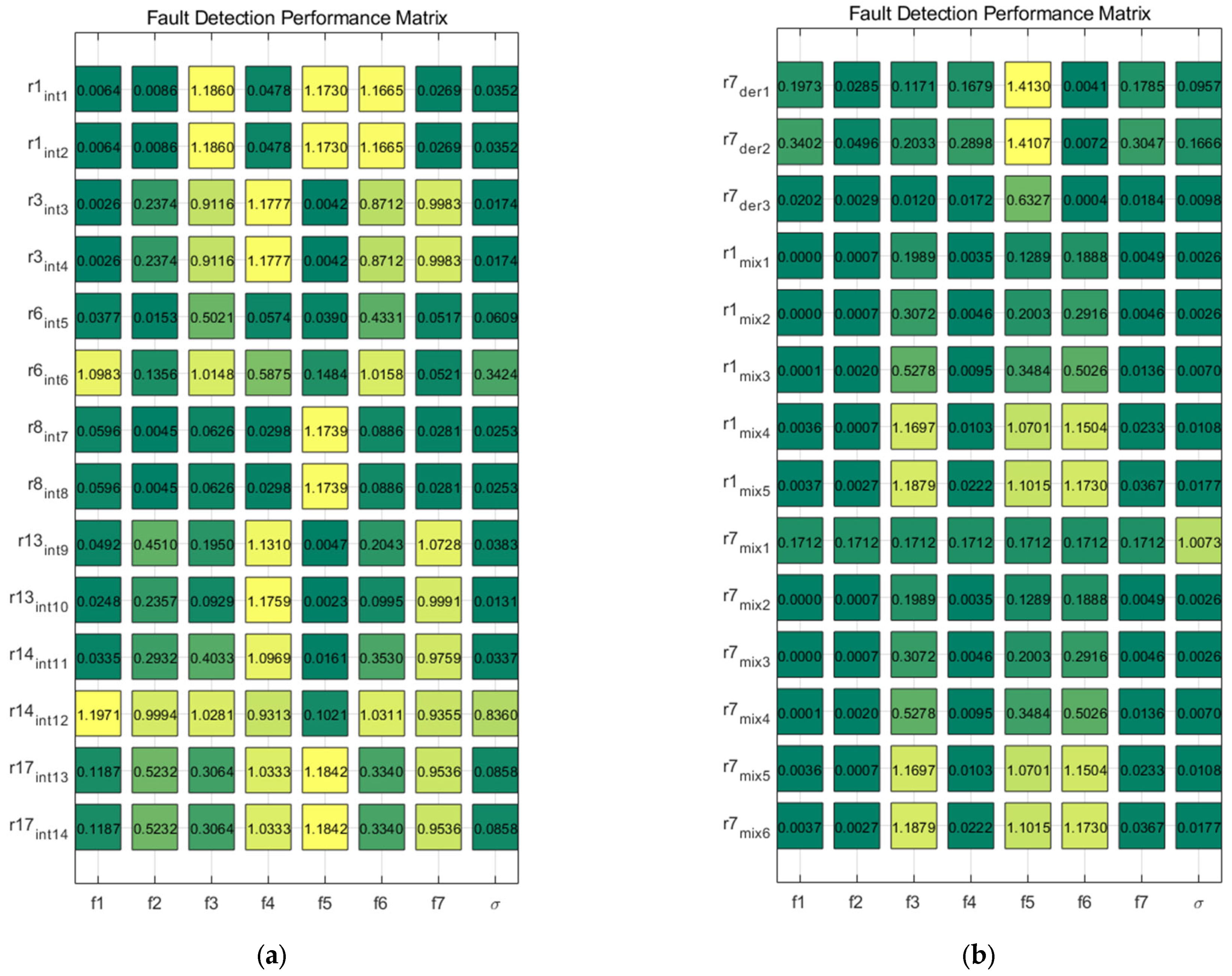
3.3. MMCD-Based Diagnosability Quantitative Assessment

Structural analysis can only qualitatively analyze the diagnosability, so this paper proposes a quantitative assessment method based on MMCD. As shown in Figure 12, there are a total of seven integral causal MSO; namely, $intMSOs=\left\{MS{O}_1,MS{O}_3,MS{O}_6,MS{O}_8,MS{O}_{13},\right.$$\left.MS{O}_{14},MS{O}_{17}\right\}$. As shown in Figure 10, two integral causal residuals can be designed for each integral causal MSO. The integral causal residual of the $intMSOs$ is $R_{\mathrm{int}}=\left\{r{1}_{\mathrm{int}1},r{1}_{\mathrm{int}2},r{3}_{\mathrm{int}3},r{3}_{\mathrm{int}4},r{6}_{\mathrm{int}5},r{6}_{\mathrm{int}6},r{8}_{\mathrm{int}7},r{8}_{\mathrm{int}8},r{13}_{\mathrm{int}9},\right.$$\left.r{13}_{\mathrm{int}10},r{14}_{\mathrm{int}11},r{14}_{\mathrm{int}12},r{17}_{\mathrm{int}13},r{17}_{\mathrm{int}14}\right\}$. Based on MMCD, the fault detection matrix $D_1$ for $R_{\mathrm{int}}$ can be obtained, as shown in Figure 17a. The first seven columns reflect the faults, the final column represents the diagnosability limit ($\sigma$), and the rows of $D_1$ represent the residuals. For example, $D_1\left(r{1}_{\mathrm{int}1},f_1\right)=0.0064$ represents the diagnosability of $r{1}_{\mathrm{int}1}$ for $f_1$, and $D_1\left(r{1}_{\mathrm{int}1},\sigma \right)=0.00352$ represents the diagnosability limit of $r{1}_{\mathrm{int}1}$. As $D_1\left(r{1}_{\mathrm{int}1},\sigma \right)>D_1\left(r{1}_{\mathrm{int}1},f_1\right)$, $r{1}_{\mathrm{int}1}$ cannot diagnose $f_1$. Further, as $D_1\left(r{1}_{\mathrm{int}1},f_3\right)>D_1\left(r{1}_{\mathrm{int}1},f_5\right)>D_1\left(r{1}_{\mathrm{int}1},f_6\right)>D_1\left(r{1}_{\mathrm{int}1},f_4\right)>D_1\left(r{1}_{\mathrm{int}1},\sigma \right)>D_1\left(r{1}_{\mathrm{int}1},f_7\right)>$$D_1\left(r{1}_{\mathrm{int}1},f_2\right)>$$D_1\left(r{1}_{\mathrm{int}1},f_1\right)$, $r{1}_{\mathrm{int}1}$ can diagnose $\left\{f_3,f_4,f_5,f_6\right\}$. The sensitivity of $r{1}_{\mathrm{int}1}$ to the faults is $f_3>f_5>f_6>f_4$. From a qualitative point of view, $r{1}_{\mathrm{int}1}$ cannot diagnose fault $f_4$. However, a coupling relationship exists between the states. When a fault occurs in one state, it affects the changes in other states because the fault is transmissible. Therefore, from a quantitative point of view, $r{1}_{\mathrm{int}1}$ can diagnose $f_4$. This also reflects the advantage of quantitative assessment.

As shown in Figure 17a, comparing the fault diagnostic values of the residuals of the same MSO design, it can be found that the diagnosability is the same for the integrally causal residuals based on $\left\{MS{O}_1,MS{O}_3,MS{O}_8,MS{O}_{17}\right\}$. However, the diagnosability of the integrally causal residuals based on $\left\{MS{O}_6,MS{O}_{13},MS{O}_{14}\right\}$ designs is different. For comparative analysis, the mixed causal residual $R{1}_{mix}=\left\{r{1}_{mix1},r{1}_{mix2},r{1}_{mix3},r{1}_{mix4},r{1}_{mix5}\right\}$ is designed based on $MS{O}_1$. The differentially causal residual $R{7}_{der}=\left\{r{7}_{der1},r{7}_{der2},r{7}_{der3}\right\}$ and the mixed causal residual $R{7}_{mix}=\left\{r{7}_{mix1},r{7}_{mix2},r{7}_{mix3},r{7}_{mix4},r{7}_{mix5},r{7}_{mix6}\right\}$ are designed based on $MS{O}_7$. The fault diagnosis matrix $D_2$ for residual $\left\{R{1}_{\mathrm{mi}x},R{7}_{der},R{7}_{mix}\right\}$ is shown in Figure 17b. The comparative analysis reveals that the fault diagnosis capabilities of $R{1}_{mix}$, $R{7}_{der}$, and $R{7}_{mix}$ are different. Therefore, most of the fault diagnosis capabilities in the same causal residuals based on the same MSO design are inconsistent.

To further verify the effect of causality on diagnosability, here, based on $MS{O}_1$, $e_6$, $e_8$, and $e_{10}$ are selected as redundant equations, and the differential causal residuals $r{1}_{der}$, the mixed causal residuals $r{1}_{mix}$, and the integral causal residuals $r{1}_{\mathrm{int}}$ are sequentially designed. The fault diagnostic capability matrix $D_3$ of $\left\{r{1}_{der},r{1}_{mix},r{1}_{\mathrm{int}}\right\}$ is shown in Figure 17c. As $\left|D_3\left(r{1}_{\mathrm{int}},f_3\right)-D_3\left(r{1}_{\mathrm{int}},\sigma \right)\right|>$$\left|D_3\left(r{1}_{mix},f_3\right)\right.$$\left.-D_3\left(r{1}_{mix},\sigma \right)\right|>$$\left|D_3\left(r{1}_{der},f_3\right)-D_3\left(r{1}_{der},\sigma \right)\right|$, the fault diagnosis capability of $r{1}_{\mathrm{int}}$ is more potent than that of $r{1}_{der}$ and $r{1}_{mix}$. Therefore, the influence of causality must be taken into account in the design of the diagnostic system.

When $R_1=\left\{r{1}_{\mathrm{int}1},r{1}_{\mathrm{int}2},r{3}_{\mathrm{int}3},r{3}_{\mathrm{int}4}\right\}$ in Figure 17a is selected as the diagnostic system, the fault diagnosis matrix $D_4$ of $R_1$ is displayed in Figure 17d. Here, the detectability limit ${\sigma }_{D_1}=0.0555$, and the isolability limit ${\sigma }_{I_1}=0$. As $D_4\left(f_4,NF\right)>D_4\left(f_5,NF\right)>$$D_4\left(f_3,NF\right)>D_4\left(f_6,NF\right)>D_4\left(f_7,NF\right)>D_4\left(f_2,NF\right)>{\sigma }_{D_1}>D_4\left(f_1,NF\right)$, $R_1$ can diagnose all faults except $f_1$, which is consistent with the sensitivity of $MS{O}_1$ and $MS{O}_3$ to faults, as shown in Figure 12a. The fault detection rate of $R_1$ is $FD{R}_7=85.71\%$. As fault diagnosis is a prerequisite for fault isolation, $D_4\left(f_1,\cdot \right)>{\sigma }_{I_1}$ and $D_4\left(\cdot ,f_1\right)>{\sigma }_{I_1}$ are meaningless. As $D_4\left(f_i,f_j\right)>{\sigma }_{I_1}$, $i\ne j$, and $i,j=2,\dots ,7$, the fault isolation rate of $R_1$ is $FI{R}_7=71.43\%$. As shown in Figure 11a, from a qualitative assessment point of view, $R_1$ does not guarantee that the faults $\left\{f_2,f_4,f_7\right\}$ are isolated from each other or that the faults $\left\{f_3,f_6\right\}$ are isolated from each other. However, from the perspective of quantitative assessment, the faults in $\left\{f_3,f_6\right\}$ and $\left\{f_2,f_4,f_7\right\}$ are isolated from each other. As shown in Figure 16, the sensitivity of the same residuals to different faults and the degree of jump of different residuals when the same fault occurs are different. Based on MMCD, this difference can be quantitatively characterized, which is not possible with qualitative assessment.

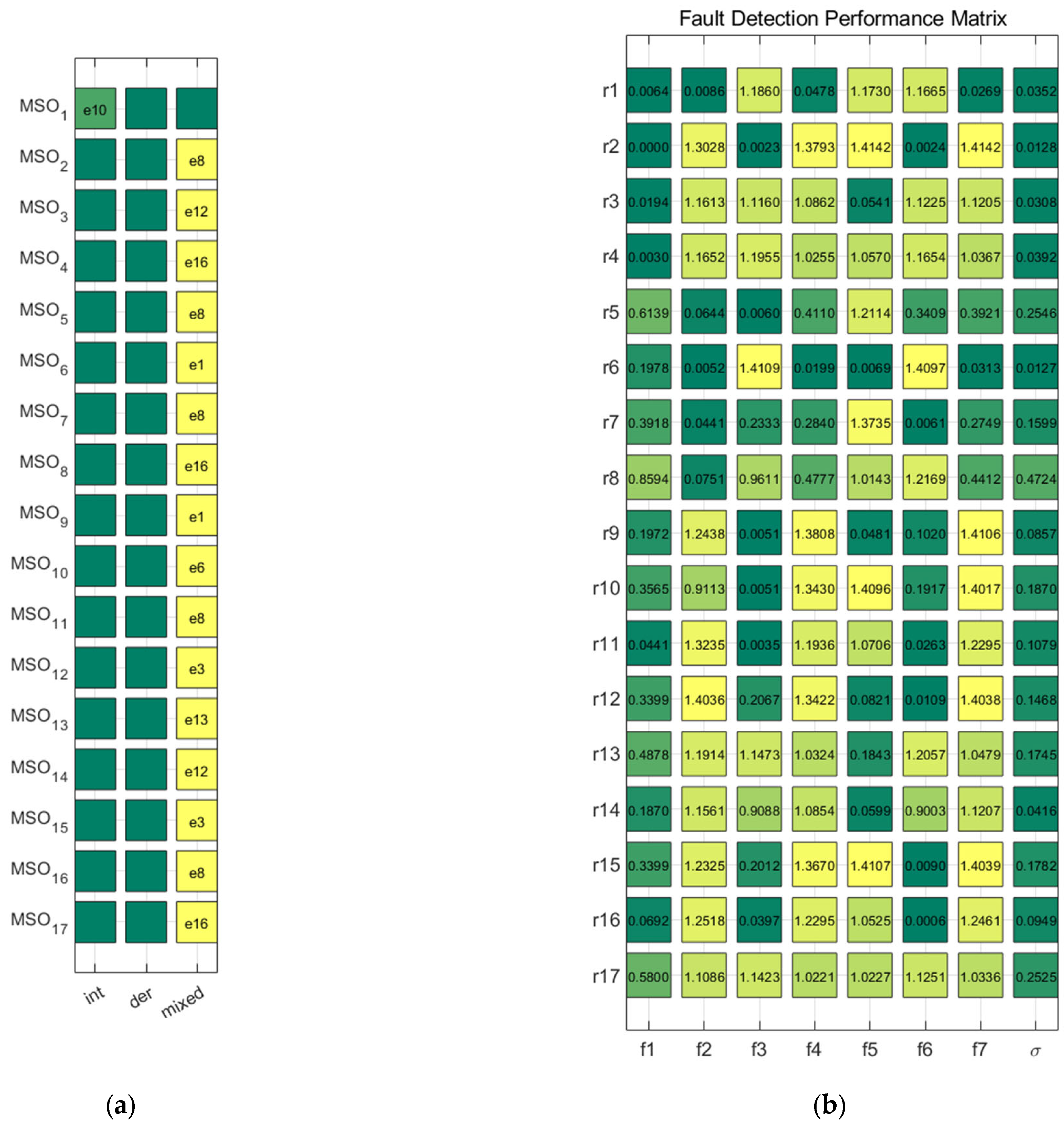
3.4. Diagnosability Optimization Design Based on the GWO Algorithm

To fully consider the causal diagnosability difference of the residuals of the same MSO design, it is necessary to determine the residuals with the most considerable diagnosability ability in the residual set of the same MSO design based on MMCD before optimization of the diagnosability design. First, based on each $MS{O}_i=\left\{e_j\right\}$ in $MSOs=\left\{MS{O}_1,MS{O}_2,\dots ,MS{O}_{17}\right\}$, take any one of the equations $e_j$ design residuals $R_i=\left\{r_{ij}\right\}$ in turn. Second, based on MMCD, calculate the fault detection matrix $D_i$ of $R_i$. Then, calculate the fault diagnostic capability $D_{r_{ij}}=\left\{d_{r_{ij}}\right\}$ of the residual $R_i=\left\{r_{ij}\right\}$.

$$d_{r_{ij}}={\displaystyle \sum _{k=1}^7\epsilon \left(D_i\left(r_{ij},f_k\right)-{\sigma }_{r_{ij}}\right)}$$

(41)

Here,

$$\epsilon \left(\alpha \right)=\left\{\begin{array}{l}\left|\alpha \right|, if \alpha >0\hfill \\ 0, otherwise\hfill \end{array}\right.$$

(42)

Then, the residual $r_i$ corresponding to the maximum value $\max \left\{D_{r_{ij}}\right\}$ in $D_{r_{ij}}$ is found. Finally, the set of candidate residuals is obtained as $R_{con}=\left\{r_1,r_2,\dots ,r_{17}\right\}$. The causality of $R_{con}$ and the selected redundancy equations are shown in Figure 18a, and Figure 18b displays its fault diagnosis performance matrix $D_6$. The matrix $D_5$, as shown in Figure 18a, has rows representing each MSO and columns representing causality. For example, $D_5\left(MS{O}_1,\mathrm{int}\right)=e_{10}$ indicates that when $MS{O}_1$ chooses $e_{10}$ as the redundant equation, the diagnostic performance of the designed residual is maximized, and the residual is integrally causal. Here, the optimal residuals are mixed causal except for the optimal residuals of $MS{O}_1$, which are integrally causal.

To fulfill the diagnosability and the cost of the diagnostic system, this paper uses the diagnosability optimization design strategy based on the GWO algorithm and selects the residual set $R$ of $R_{con}$ with the best comprehensive performance. For comparison and evaluation, this study employs the simulated annealing (SA), genetic (GA), and sine-cosine (SCA) algorithms for analysis. Let ${\gamma }_i=1$, and the diagnosability optimization results are illustrated in Figure 19.

Figure 19a shows the fitness curves of each algorithm. The GWO algorithm achieves the optimal value in the second iteration, which is advantageous in terms of the optimization searching speed compared with other algorithms. In terms of optimization accuracy, both the GWO algorithm and the SCA achieved the optimal value. Figure 19b,c show the FSM and FIM of the MSO corresponding to the optimized residuals. Combined with Figure 18a, it can be observed that the GWO algorithm optimizes the $\left\{MS{O}_1,MS{O}_2,MS{O}_7,MS{O}_9,MS{O}_{14}\right\}$ to design the residuals $R=\left\{r_1,r_2,r_7,r_9,r_{14}\right\}$, and all the residuals are mixed causal except for $r_1$, which is integrally causal. From a qualitative assessment point of view, based on Figure 19b, $FD{R}_8=100\%$ can be obtained. Based on Figure 19c, $FI{R}_8=85.71\%$ can be obtained.

Using MMCD, the quantitative assessment matrix $D_7$ of $\left\{r_1,r_2,r_7,r_9,r_{14}\right\}$ can be obtained as shown in Figure 19d, where the detectability limit ${\sigma }_{D_2}=0.1891$ and the isolation limit ${\sigma }_{I_1}=0.0428$. Based on $D_7$ and Equation (27), its fault diagnosis matrix $D_8$ is established as shown in Figure 19e. Therefore, from the perspective of quantitative assessment, $FD{R}_9=100\%$ and $FI{R}_9=100\%>FI{R}_8$ can be obtained. Comparing Figure 19e with Figure 19c, it is observed that $\left\{f_2,f_4,f_7\right\}$ are not isolated from each other in the qualitative assessment. However, in the quantitative assessment, they can indeed be isolated. This is mainly due to the fact that the residuals are not sensitive to the faults. From the causality of the optimized residuals, it can be seen that mixed causality accounts for 80% of the residuals, which further reflects the advantage of mixed causality. From the results of the quantitative optimization, the overall cost of optimization is reduced by 70.59%, and the system achieves a 100% fault detection rate and fault isolation rate. This further demonstrates the advantages of the quantitative assessment.

4. Summary

To improve UAV reliability and diagnosability, this study suggested a causal diagnosability optimization design approach based on the MMCD and GWO algorithms. First, this study offers a qualitative approach to causal diagnosability evaluation based on structural analysis; second, to measure the ease of fault diagnosis, it presents a quantitative approach to causal diagnosability evaluation using the MMCD; and third, to balance the need for diagnosability and the cost of diagnostic system design, it suggests a design strategy to maximize causal diagnosability using the GWO algorithm. According to simulation findings, the enhanced diagnostic system maintains 100% fault isolation and detection rates while reducing design costs by 70.59%.

Furthermore, the findings of the causal diagnosability evaluation indicate that, first, the diagnosability varies depending on the causality. Under mixed causal constraints, diagnosability performs the best among them. Second, different evaluation techniques have various diagnoses. This is mostly because faults and residuals have different sensitivity levels, and the quantitative evaluation successfully captures and quantifies these sensitivity variations. This explains why the quantitative assessment isolates flaws that the qualitative review cannot identify.

Future studies might examine how interference and noise affect diagnosability. Furthermore, optimizing the diagnosability of the structurally precise and poorly defined subsystems is possible.

References

1. Mohsan, S.A.H.; Khan, M.A.; Noor, F.; Ullah, I.; Alsharif, M.H. Towards the Unmanned Aerial Vehicles (UAVs): A Comprehensive Review. Drones 2022, 6, 147. [Google Scholar] [CrossRef]
2. del Cerro, J.; Cruz Ulloa, C.; Barrientos, A.; de León Rivas, J. Unmanned Aerial Vehicles in Agriculture: A Survey. Agronomy 2021, 11, 203. [Google Scholar] [CrossRef]
3. Ghamari, M.; Rangel, P.; Mehrubeoglu, M.; Tewolde, G.S.; Sherratt, R.S. Unmanned Aerial Vehicle Communications for Civil Applications: A Review. IEEE Access 2022, 10, 102492–102531. [Google Scholar] [CrossRef]
4. Zuo, Z.; Liu, C.; Han, Q.-L.; Song, J. Unmanned Aerial Vehicles: Control Methods and Future Challenges. IEEE/CAA J. Autom. Sin. 2022, 9, 601–614. [Google Scholar] [CrossRef]
5. Gu, X.; Shi, X. A review of research on diagnosability of control systems. Energy Rep. 2024, 11, 2174–2188. [Google Scholar] [CrossRef]
6. Fourlas, G.K.; Karras, G.C. A Survey on Fault Diagnosis Methods for UAVs. In Proceedings of the 2021 International Conference on Unmanned Aircraft Systems (ICUAS), Athens, Greece, 15–18 June 2021; pp. 394–403. [Google Scholar] [CrossRef]
7. Fourlas, G.K.; Karras, G.C. A Survey on Fault Diagnosis and Fault-Tolerant Control Methods for Unmanned Aerial Vehicles. Machines 2021, 9, 197. [Google Scholar] [CrossRef]
8. Iannace, G.; Ciaburro, G.; Trematerra, A. Fault Diagnosis for UAV Blades Using Artificial Neural Network. Robotics 2019, 8, 59. [Google Scholar] [CrossRef]
9. Liang, S.; Zhang, S.; Huang, Y.; Zheng, X.; Cheng, J.; Wu, S. Data-driven fault diagnosis of FW-UAVs with consideration of multiple operation conditions. ISA Trans. 2022, 126, 472–485. [Google Scholar] [CrossRef]
10. Zhang, Y.; Li, S.; Zhang, A.; An, X. FW-UAV fault diagnosis based on knowledge complementary network under small sample. Mech. Syst. Signal Process. 2024, 215, 111418. [Google Scholar] [CrossRef]
11. Hua, L.; Zhang, J.; Li, D.; Xi, X.; Shah, M.A. Sensor Fault Diagnosis and Fault Tolerant Control of Quadrotor UAV Based on Genetic Algorithm. J. Sens. 2022, 2022, 8626722. [Google Scholar] [CrossRef]
12. Gu, X.; Shi, X. A Review of Research on Diagnosability of Control Systems Based on Structural Analysis. Appl. Sci. 2023, 13, 12241. [Google Scholar] [CrossRef]
13. Chen, Z.; Xu, J.; Peng, T.; Yang, C. Graph Convolutional Network-Based Method for Fault Diagnosis Using a Hybrid of Measurement and Prior Knowledge. IEEE Trans. Cybern. 2022, 52, 9157–9169. [Google Scholar] [CrossRef] [PubMed]
14. Cheng, Y.; D’Arpino, M.; Rizzoni, G. Fault Diagnosis in Lithium-ion Battery of Hybrid Electric Aircraft based on Structural Analysis. In Proceedings of the 2022 IEEE Transportation Electrification Conference & Expo (ITEC), Anaheim, CA, USA, 15–17 June 2022; pp. 997–1004. [Google Scholar] [CrossRef]
15. Li, X.; Xu, J.; Chen, Z.; Xu, S.; Liu, K. Real-Time Fault Diagnosis of Pulse Rectifier in Traction System Based on Structural Model. IEEE Trans. Intell. Transp. Syst. 2022, 23, 2130–2143. [Google Scholar] [CrossRef]
16. Yin, C.; He, Z.; Wang, J.; Zhou, H. A method for fault diagnosability evaluation of spacecraft control system. In Proceedings of the 2016 Joint International Information Technology, Mechanical and Electronic Engineering, Xi’an, China, 4–5 October 2016; Xu, B., Chen, Y.N., Zhao, L.H., Eds.; Atlantis Press: Paris, France, 2016; Volume 59, pp. 611–614. [Google Scholar]
17. Cui, Y.; Shi, J.; Wang, Z. System-level operational diagnosability analysis in quasi real-time fault diagnosis: The probabilistic approach. J. Process Control 2014, 24, 1444–1453. [Google Scholar] [CrossRef]
18. Cheng, Y.; Liu, Y.; Yang, S.; Wu, J. Multi-sensor optimal placement of rotor-bearing system based on fault diagnosability. Proc. Inst. Mech. Eng. Part C J. Mech. Eng. Sci. 2023, 237, 1510–1521. [Google Scholar] [CrossRef]
19. Reppa, V.; Timotheou, S.; Polycarpou, M.M.; Panayiotou, C. Performance Index for Optimizing Sensor Fault Detection of a Class of Nonlinear Systems. IFAC-PapersOnLine 2018, 51, 1387–1394. [Google Scholar] [CrossRef]
20. Fu, F.; Xue, T.; Wu, Z.; Wang, D. A Fault Diagnosability Evaluation Method for Dynamic Systems Without Distribution Knowledge. IEEE Trans. Cybern. 2022, 52, 5113–5123. [Google Scholar] [CrossRef]
21. Wang, Z.; Tang, Z.; Chen, F. Quantitative Evaluation of Sensor Fault Diagnosability of F-16 High Maneuvering Fighter. In Proceedings of the 2022 IEEE 5th International Conference on Automation, Electronics and Electrical Engineering (AUTEEE), Shenyang, China, 18–20 November 2022; pp. 102–108. [Google Scholar] [CrossRef]
22. Liu, Q.; Wang, Z.; Zhang, J.; Zhou, D. Necessary and Sufficient Conditions for Fault Diagnosability of Linear Open- and Closed-Loop Stochastic Systems Under Sensor and Actuator Faults. IEEE Trans. Autom. Control 2022, 67, 4178–4185. [Google Scholar] [CrossRef]
23. Qu, R.; Jiang, B.; Cheng, Y. Research on the Diagnosability of a Satellite Attitude Determination System on a Fault Information Manifold. Appl. Sci. 2022, 12, 12835. [Google Scholar] [CrossRef]
24. Stiefelmaier, J.; Gienger, A.; Böhm, M.; Sawodny, O.; Tarín, C. A Bayesian Approach to Fault Diagnosability Analysis in Adaptive Structures. IFAC-PapersOnLine 2022, 55, 347–352. [Google Scholar] [CrossRef]
25. Zhang, W.; Zhang, X.; Lan, L.; Luo, Z. Maximum Mean and Covariance Discrepancy for Unsupervised Domain Adaptation. Neural Process Lett. 2020, 51, 347–366. [Google Scholar] [CrossRef]
26. Yang, C.; Jia, M.; Li, Z.; Gabbouj, M. Enhanced hierarchical symbolic dynamic entropy and maximum mean and covariance discrepancy-based transfer joint matching with Welsh loss for intelligent cross-domain bearing health monitoring. Mech. Syst. Signal Process. 2022, 165, 108343. [Google Scholar] [CrossRef]
27. Gu, X.; Shi, X. Diagnosability-optimization design of fixed-wing unmanned aerial vehicle based on causal matching and tree seed algorithm. Meas. Control 2024, 00202940241307629. [Google Scholar] [CrossRef]
28. Katoch, S.; Chauhan, S.S.; Kumar, V. A review on genetic algorithm: Past, present, and future. Multimed. Tools Appl. 2021, 80, 8091–8126. [Google Scholar] [CrossRef]
29. Cunha, M.; Marques, J. A New Multiobjective Simulated Annealing Algorithm—MOSA-GR: Application to the Optimal Design of Water Distribution Networks. Water Resour. Res. 2020, 56, e2019WR025852. [Google Scholar] [CrossRef]
30. Li, W.; Yan, X.; Huang, Y. Cooperative-Guided Ant Colony Optimization with Knowledge Learning for Job Shop Scheduling Problem. Tsinghua Sci. Technol. 2024, 29, 1283–1299. [Google Scholar] [CrossRef]
31. Gad, A.G. Particle Swarm Optimization Algorithm and Its Applications: A Systematic Review. Arch. Comput. Methods Eng. 2022, 29, 2531–2561. [Google Scholar] [CrossRef]
32. Kaya, E.; Gorkemli, B.; Akay, B.; Karaboga, D. A review on the studies employing artificial bee colony algorithm to solve combinatorial optimization problems. Eng. Appl. Artif. Intell. 2022, 115, 105311. [Google Scholar] [CrossRef]
33. Qiu, Y.; Yang, X.; Chen, S. An improved gray wolf optimization algorithm solving to functional optimization and engineering design problems. Sci. Rep. 2024, 14, 14190. [Google Scholar] [CrossRef]
34. Pan, H.; Chen, S.; Xiong, H. A high-dimensional feature selection method based on modified Gray Wolf Optimization. Appl. Soft Comput. 2023, 135, 110031. [Google Scholar] [CrossRef]
35. Wang, J.; Xu, Y.-P.; She, C.; Xu, P.; Bagal, H.A. Optimal parameter identification of SOFC model using modified gray wolf optimization algorithm. Energy 2022, 240, 122800. [Google Scholar] [CrossRef]
36. Emary, E.; Zawbaa, H.M.; Grosan, C. Experienced Gray Wolf Optimization Through Reinforcement Learning and Neural Networks. IEEE Trans. Neural Netw. Learn. Syst. 2018, 29, 681–694. [Google Scholar] [CrossRef] [PubMed]
37. Kumar, A.; Pant, S.; Ram, M. System Reliability Optimization Using Gray Wolf Optimizer Algorithm. Qual. Reliab. Eng. Int. 2017, 33, 1327–1335. [Google Scholar] [CrossRef]
38. Dulmage, A.L.; Mendelsohn, N.S. Coverings of Bipartite Graphs. Can. J. Math. 1958, 10, 517–534. [Google Scholar] [CrossRef]
39. Krysander, M.; Aslund, J.; Nyberg, M. An Efficient Algorithm for Finding Minimal Overconstrained Subsystems for Model-Based Diagnosis. IEEE Trans. Syst. Man Cybern. A 2008, 38, 197–206. [Google Scholar] [CrossRef]
40. Gu, X.; Shi, X. Diagnosability-optimized design of unmanned aerial vehicles based on structural analysis and maximum mean covariance differences. Measurement 2024, 238, 115334. [Google Scholar] [CrossRef]
Figure 1. The logical lineage of the proposed strategy.
Mca 30 00055 g001
Figure 2. The structural model of  M 1 .
Mca 30 00055 g002
Figure 3. DM decomposition. (a) DM decomposition diagram. (b) DM decomposition of  M 1 .
Mca 30 00055 g003
Figure 4. Differential causal residual  r 1 . (a) The computation flow of  r 1 . (b) Differential matching.
Mca 30 00055 g004
Figure 5. Differential causal residual  r 2 . (a) The computation flow of  r 2 . (b) Integral matching.
Mca 30 00055 g005
Figure 6. Causal relation of  M S O 2 . (a) Mixed causality. (b) Integral causality. (c) Differential causality.
Mca 30 00055 g006
Figure 7. Fault signature matrix of  M 1 . (a) Integral causality. (b) Differential causality. (c) Mixed causality.
Mca 30 00055 g007
Figure 8. Fault isolability matrix of  M 1 . (a) Integral causality. (b) Differential causality. (c) Mixed causality.
Mca 30 00055 g008
Figure 9. The structural analysis of  M U A V . (a) Structural model. (b) DM decomposition.
Mca 30 00055 g009
Figure 10. The MSOs and causality of  M U A V .
Mca 30 00055 g010
Figure 11. The causal matching relationships of  M S O 1 . (a) Differential causal matching. (b) Mixed causal matching. (c) Integral causal matching.
Mca 30 00055 g011
Figure 12. Diagnosability analysis results of  i n t M S O s . (a) Fault signature matrix. (b) Fault isolation matrix.
Mca 30 00055 g012
Figure 13. Diagnosability analysis results of  d e r M S O s . (a) Fault signature matrix. (b) Fault isolation matrix.
Mca 30 00055 g013
Figure 14. Diagnosability analysis results of  m i x M S O s . (a) Fault signature matrix. (b) Fault isolation matrix.
Mca 30 00055 g014
Figure 15. Simulation run results for  M U A V . (a) Normal operation. (b f 2  occurs.
Mca 30 00055 g015
Figure 16. Diagnosability impact factor analysis. (a) Fault. (b) Causality. (c) MSO. (d) Residual.
Mca 30 00055 g016
Figure 17. MMCD-based quantitative assessment of diagnosability. (a) Integral causality. (b) Differential and mixed causation. (c) Causal comparison. (d) Diagnosability quantitative assessment.
Mca 30 00055 g017aMca 30 00055 g017b
Figure 18. Causal diagnosability of  R c o n . (a) Causality. (b) Fault diagnosis matrix of  R c o n .
Mca 30 00055 g018
Figure 19. Diagnosability optimization results based on the GWO algorithm. (a) Fitness curves. (b) Fault signature matrix. (c) Fault isolation matrix. (d) Diagnosability quantitative assessment matrix. (e) Fault diagnosis matrix.
Mca 30 00055 g019
Disclaimer/Publisher’s Note: The statements, opinions and data contained in all publications are solely those of the individual author(s) and contributor(s) and not of MDPI and/or the editor(s). MDPI and/or the editor(s) disclaim responsibility for any injury to people or property resulting from any ideas, methods, instructions or products referred to in the content.