Penalty Strategies in Semiparametric Regression Models

Abstract

This study includes a comprehensive evaluation of six penalty estimation strategies for partially linear models (PLRMs), focusing on their performance in the presence of multicollinearity and their ability to handle both parametric and nonparametric components. The methods under consideration include Ridge regression, Lasso, Adaptive Lasso (aLasso), smoothly clipped absolute deviation (SCAD), ElasticNet, and minimax concave penalty (MCP). In addition to these established methods, we also incorporate Stein-type shrinkage estimation techniques that are standard and positive shrinkage and assess their effectiveness in this context. To estimate the PLRMs, we consider a kernel smoothing technique grounded in penalized least squares. Our investigation involves a theoretical analysis of the estimators’ asymptotic properties and a detailed simulation study designed to compare their performance under a variety of conditions, including different sample sizes, numbers of predictors, and levels of multicollinearity. The simulation results reveal that aLasso and shrinkage estimators, particularly the positive shrinkage estimator, consistently outperform the other methods in terms of Mean Squared Error (MSE) relative efficiencies (RE), especially when the sample size is small and multicollinearity is high. Furthermore, we present a real data analysis using the Hitters dataset to demonstrate the applicability of these methods in a practical setting. The results of the real data analysis align with the simulation findings, highlighting the superior predictive accuracy of aLasso and the shrinkage estimators in the presence of multicollinearity. The findings of this study offer valuable insights into the strengths and limitations of these penalty and shrinkage strategies, guiding their application in future research and practice involving semiparametric regression.

1. Introduction

The Partially Linear Regression Model (PLRM), introduced by [1], serves as a versatile tool for utilizing the advantage of both parametric linear models and nonparametric regression models. It allows for the modeling of complex relationships by incorporating both linear and nonlinear components, thereby offering greater flexibility and interpretability across various scientific disciplines, including social sciences, biology, and economics. Formally, the PLRM is defined as:

$$y_i={\mathbf{x}}_i^{\prime }\mathsf{\beta }+f\left(t_i\right)+{\epsilon }_i, i=1,\dots ,n$$

(1)

where $y_i\prime s$ are the observations of the response variable, ${\mathbf{x}}_i=(x_{i1},\dots ,x_{ik})$ and $t_i\prime s$ are the values of the explanatory variable, $\mathsf{\beta }={({\beta }_1,\dots ,{\beta }_k)}^{\prime }$ is an unknown k-dimensional parameter vector to be estimated, $f\left(.\right)$ is an unknown smooth function, and ${\epsilon }_i\prime s$ are assumed to be uncorrelated random variables with mean zero and a common variance ${\sigma }^2$ and independent of the explanatory variables. Note also that the observations of $y_i$ depend linearly on the entries of ${\mathbf{x}}_i$ and nonlinearly on the values of a univariate variable $t_i$. The PLRM can be re-expressed in matrix and vector form:

$$\mathbf{y}=\mathbf{X}\mathsf{\beta }+\mathbf{f}+\mathit{\epsilon }$$

(2)

where $\mathbf{y}={\left(y_1,\dots ,y_n\right)}^{\prime }$, $\mathbf{X}={[{\mathbf{x}}_1,\dots ,{\mathbf{x}}_n]}^{\prime }$ is an ($n\times k$) design matrix with ${{\mathbf{x}}_i=(x_{i1},\dots ,x_{ik})}^{\prime }$ denoting the i.th$k-$dimensional row vector of the design matrix X, and $\mathbf{f}={\left(f\left(t_1\right),\dots ,f\left(t_n\right)\right)}^{\prime }$ and $\mathsf{\epsilon }=\left({\epsilon }_1,.{\epsilon }_2,\dots ,{\epsilon }_n\right)$ are random error vectors with $E\left(\mathit{\epsilon }\right)=0$ and $Var\left(\mathit{\epsilon }\right)={\mathsf{\sigma }}^2{\mathbf{I}}_n$. For more discussion on Model (1), see [2,3,4], among others. Since it was initially presented in [1], this model has been very popular and is frequently used in the social, biological, and economic sciences. The PLRM generalizes both the parametric linear regression model and nonparametric regression model. When the $\mathbf{f}=0$, Model (1) reduces to the linear regression model $y_i={\mathbf{x}}_i\mathsf{\beta }+{\epsilon }_i$, when the $\mathsf{\beta }=0$ model (1) becomes a nonparametric regression model

$$y_i=f\left(t_i\right)+{\epsilon }_i$$

(3)

with a univariate covariate. In addition, because PLRMs contain both linear and nonlinear components, they are more flexible than linear models. In this work, we are interested in estimating parameter vector $\mathsf{\beta }$ and function $\mathbf{f}$.

Estimating the parameters and the smooth function in PLRM has been a focal point of research, with various methodologies proposed to enhance estimation accuracy and model interpretability. Early contributions [4,5] utilized kernel smoothing techniques for estimating the nonparametric component, laying the groundwork for subsequent advancements.

The advent of regularization methods introduced in [6,7] revolutionized parameter estimation by addressing issues such as multicollinearity and high-dimensionality through penalty functions. In particular, the authors of [8,9] explored penalized least squares in semiparametric models, emphasizing the integration of penalty functions with kernel smoothing to enhance estimator performance (see also [10,11,12,13]).

Adaptive methods, such as the Adaptive Lasso (aLasso) introduced in [14], have been incorporated into PLRM frameworks to improve variable selection consistency. Moreover, SCAD [15] and MCP [16] penalties have been employed to mitigate the bias inherent in $L_1$ penalties, providing more accurate parameter estimates in complex models. Recent studies [17,18] highlight the asymptotic properties of penalized estimators in semiparametric regression, emphasizing the significance of penalty strategies in PLRM. Challenges in balancing bias and variance persist, particularly in sparsity contexts with multicollinearity.

In regression problems, multicollinearity emerges when variables are highly correlated with each other and the dependent variable. This situation inflates confidence intervals, weakens parameter estimates, and leads to less reliable predictions. It also raises sampling variance, reducing accuracy for both inference and prediction. To counter these challenges in PLRMs, we integrate shrinkage estimation with penalty functions to bolster robustness and manage both multicollinearity and variable selection:

• We tackle variable selection and multicollinearity in Model (1), which features strongly correlated covariates, using six penalty functions: Ridge, Lasso, aLasso, SCAD, Elastic Net, and MCP.
• We then review and compare these methods, highlighting their strengths, limitations, and uses within PLRMs.
• To further enhance parameter estimation, we incorporate shrinkage estimation techniques—both standard and positive shrinkage estimators—into the penalty-based framework.
• Finally, kernel smoothing via penalized least squares is employed to estimate both the parametric (linear) and nonparametric (smooth) components of the model.

The remainder of this paper is structured as follows. At the end of this section, we summarized the background on penalty functions and partially linear models and their integration. Section 2 describes the kernel smoothing method. Section 3 introduces the kernel-type ridge estimator. In Section 4, we discuss penalty functions and shrinkage estimators based on kernel smoothing. Section 5 presents the evaluation metrics for both parametric and nonparametric components. Section 6 outlines the estimators’ asymptotic properties. Section 7 details the Monte Carlo simulations. Section 8 compares the performance of our proposed estimators on real data. Finally, Section 9 provides concluding remarks and includes supplementary technical materials.

Background

In this section, we present a relevant literature review of partially linear regression models (PLRMs) and show why penalty functions and shrinkage estimators are essential for handling challenges like multicollinearity, high-dimensional data, and complex nonlinearities. We also explain how kernel smoothing complements these approaches by capturing intricate patterns in the data based on the previous studies. Altogether, these methods offer a strong foundation for building reliable and flexible statistical models.

Partially Linear Regression Models (PLRMs) are a cornerstone of semiparametric statistics, offering a powerful way to model relationships that are not fully captured by purely parametric or nonparametric approaches. They blend the interpretability of linear models with the flexibility of nonparametric methods, making them ideal for data with both linear and nonlinear components. Their ability to isolate certain covariate effects while accommodating nonlinearities has led to widespread use in fields such as economics, biostatistics, and environmental science [19]. Recent developments have expanded their scope to high-dimensional, longitudinal, and survival data [20,21].

Regularization methods, particularly those using penalty functions, have revolutionized regression analysis by tackling issues like multicollinearity, high dimensionality, and model selection. By constraining coefficient magnitudes, these methods shrink coefficients toward zero and improve model stability. Different penalty functions yield diverse estimators suited to various data characteristics and research goals.

Ridge regression, pioneered in [22], is well-established, yet its application in high-dimensional contexts and its ties to Bayesian methods continue to be studied [23]. Lasso has also evolved substantially [6], with research on its consistency in variable selection, high-dimensional settings, and extensions to generalized linear models [24]. Ahmed and colleagues contributed to Lasso’s development in PLRMs using Stein-type shrinkage estimators, especially under multicollinearity [25].

Building on the adaptive Lasso (aLasso) [26], researchers have explored data-driven weights for improving variable selection and estimation. For SCAD, recent work has focused on high-dimensional data, quantile regression, and robust estimation [27]. The researchers applied SCAD along with the other penalty functions and with shrinkage estimators in PLRMs, showing its effectiveness in handling outliers [10]. MCP, initially studied in [16], has inspired efficient algorithms and further theoretical exploration [25]. Elastic Net, proposed in [26], has also gained traction in areas like genomics, imaging, and finance, where it handles correlated predictors well [7]. Its benefits are used for balancing bias and variance in PLRMs [11].

Beyond these penalty-based approaches, shrinkage estimation techniques—particularly Stein-type estimators—offer another route. The authors of [28] investigated partially linear models by splitting the coefficient vector into main and nuisance effects and comparing shrinkage, pretest, and absolute penalty estimators. Their results show that a Stein-type shrinkage estimator uniformly outperforms the conventional least squares approach, especially when the nuisance parameter space is large, while the pretest estimator only offers benefits in a limited region. These methods shrink coefficients toward a chosen target, thereby reducing variance and mitigating noise [29,30,31]. Further, Ahmed’s work demonstrates that these techniques can improve estimation accuracy and interpretability in partially linear regression models [8,32,33]. Meanwhile, kernel smoothing remains central to nonparametric estimation for capturing nonlinear relationships, with advances such as adaptive bandwidth selection [34] and its integration with penalty and shrinkage methods [35]. The authors of [36] showed via simulation that applying Stein-type shrinkage to the parametric components of the semi-nonparametric regression model [37] enhanced accuracy. The authors of [38] proposed a two-stage approach using LASSO/Elastic-Net for variable selection followed by post-selection shrinkage estimation to improve predictions in high-dimensional sparse linear regression models, while the authors of [10] introduced shrinkage-type estimators for reliability and stress–strength parameters from progressively censored data that outperformed MLEs in simulations and industrial applications. Additional insights on shrinkage estimators are provided in [31,39,40,41,42,43,44].

Combining penalty functions with kernel smoothing has become a potent strategy for complex data in PLRMs. This approach refines the parametric part through penalty-driven selection and shrinkage, while kernel smoothing captures nonlinearities. Recent studies highlight theoretical and practical benefits, including improved estimation accuracy and consistency in variable selection under multicollinearity or high dimensionality [45]. The advanced penalized kernel smoothing in PLRMs using shrinkage estimators is shown in [32], showing strong performance in simulations and real data. That work illustrates the advantages of using penalties like aLasso and shrinkage estimation alongside kernel smoothing, especially with high-dimensional covariates and intricate nonlinearities.

2. Estimation Based on Kernel Smoothing

Let us first consider the nonparametric estimation of the unknown regression function $f\left(t\right)$ in Model (1). For simplicity, we assume that $\mathsf{\beta }$is known from Equation (1). The relationship between $y_i-{\mathbf{X}}_{\mathit{i}}\mathsf{\beta }$and $t_i$in this instance may be represented as

$$\left(y_i-{\mathbf{X}}_{\mathbf{i}}\mathsf{\beta }\right)=f\left(t_i\right)+{\epsilon }_{i, } i=1, \dots , n$$

(4)

The nonparametric part of the semiparametric model is equivalent to Equation (4). This results in the Nadaraya-Watson estimator, commonly known as the kernel estimator, which was proposed in [46,47], as mentioned in [4]:

$$\widehat{f}\left(h,t\right)={\sum }_{i=1}^n{w}_i(h, t_i)(y_i-{\mathbf{X}}_{\mathbf{i}}\mathsf{\beta })={\mathbf{W}}_h(\mathbf{y}-\mathbf{X}\mathsf{\beta })$$

(5)

where ${\mathbf{W}}_h$ is a kernel smoothing matrix with $j$-th entries${ w}_{hi}$ and where $h$ is a smoothing parameter (or bandwidth), as shown by:

$$w_i\left(h,t_i\right)=K\left({\displaystyle \frac{t-t_i}{h}}\right)/\sum _{i=1}^{n}K \left({\displaystyle \frac{t-t_i}{h}}\right)=K(u_i)/\sum _{i}K\left(u_i\right)$$

(6)

To estimate $f\left(t\right)$, kernel smoothing (regression) uses appropriate weights $w_i(h,t)$, as shown in Equation (4). The kernel function $K\left(u\right)$ with a smoothing parameter $h$, which defines the size of the neighborhood around $t$, directs the weights assigned to the observations $t_i$ [48,49]. The kernel or weight function $K\left(u\right)$ in Equation (6) has the properties of $\int K\left(u\right)du=1$ and $K\left(u\right)=K(-u)$. The kernel function is chosen to give the closest observations the most weight and the farthest from $t$the least weight.

The following partial residuals may be obtained via the matrix and vector forms of Model (2) in matrix form:

$$\mathsf{\epsilon }=\mathbf{y}-\mathbf{X}\mathsf{\beta }-\widehat{\mathbf{f}}=\left(\mathbf{I}-{\mathbf{W}}_h\right)\left(\mathbf{y}-\mathbf{X}\mathsf{\beta }\right)=\tilde{\mathbf{y}}-\tilde{\mathbf{X}}\mathsf{\beta }$$

(7)

where $\tilde{\mathbf{X}}=\left(\mathbf{I}-{\mathbf{W}}_h\right)\mathbf{X}$ and $\tilde{\mathbf{y}}=\left(\mathbf{I}-{\mathbf{W}}_h\right)\mathbf{y}.$ Hence, a transformed set of data based on kernel residuals is what we obtain as a result. The following weighted least squares (WLS) criterion is obtained by considering these partial residuals for the vector $\mathsf{\beta }$:

$$\mathbf{W}\mathbf{L}\mathbf{S}\left(\mathsf{\beta };h\right){=\left(\left(\mathbf{I}-{\mathbf{W}}_h\right)\left(\mathbf{y}-\mathbf{X}\mathsf{\beta }\right)\right)}^{\mathbf{T}}(\mathbf{I}-{\mathbf{W}}_h)(\mathbf{y}-\mathbf{X}\mathsf{\beta }{))=(\tilde{\mathbf{y}}-\tilde{\mathbf{X}}\mathsf{\beta })}^{\mathbf{\prime }}(\tilde{\mathbf{y}}-\tilde{\mathbf{X}}\mathsf{\beta })$$

(8)

The result for the criterion $\mathbf{W}\mathbf{L}\mathbf{S}\left(\mathsf{\beta };h\right)$ provided in Equation (8) is easily demonstrated to be similar to the solution of ordinary least squares (OLS)

$${{\widehat{\mathsf{\beta }}}_{KS}(h)=({\tilde{\mathbf{X}}}^{\prime }\mathbf{X})}^{-1}{\tilde{\mathbf{X}}}^{\prime }\tilde{\mathbf{y}}$$

(9)

Additionally, revising the steps for $f\left(t\right)$ reduces Equation (5) to the form:

$$\widehat{f}\left(h,t\right)=\sum _{i=1}^n{\displaystyle \frac{K\left(\frac{t-t_i}{h}\right)}{\sum _{i=1}^{n}K \left(\frac{t-t_i}{h}\right)}}(y_i-x_i\widehat{\beta })$$

(10)

Another way to express Equation (10) in a matrix is as follows:

$${\widehat{\mathbf{f}}}_{KS}={\mathbf{W}}_h(\mathbf{y}-\mathit{X}{\widehat{\mathsf{\beta }}}_{KS}).$$

(11)

Thus, our estimation for ${\mathbf{y}}_{KS}$ becomes:

$${\widehat{\mathbf{y}}}_{KS}=\mathit{X}{\widehat{\mathsf{\beta }}}_{KS}+{\widehat{\mathbf{f}}}_{KS}=\mathbf{X}({\tilde{\mathbf{X}}}^{\prime }{\tilde{\mathbf{X}})}^{-1}{\tilde{\mathbf{X}}}^{\prime }\tilde{\mathbf{y}}+{\mathbf{W}}_h(\mathbf{y}-\mathbf{X}{\widehat{\mathsf{\beta }}}_{KS})={\mathbf{H}}_{KS}\left(h\right)\mathbf{y}$$

for the hat (projection) matrix

$${\mathbf{H}}_{KS}\left(h\right)={\mathbf{W}}_h+\tilde{\mathbf{X}}{({\tilde{\mathbf{X}}}^{\prime }\mathbf{X})}^{-1}{\tilde{\mathbf{X}}}^{\prime }(\mathbf{I}-{\mathbf{W}}_h)$$

(12)

3. Kernel Type Ridge Estimator in Semiparametric Model

For the sake of this paper, we limit our attention to kernel smoothing estimators of vector parameter $\mathsf{\beta }$ and unidentified smooth function $f\left(.\right)$ in a semiparametric model. The corresponding estimators $\mathsf{\beta }$ and $\mathbf{f}$ are based on Model (2) for a given bandwidth parameter $h$. By multiplying $\left({\mathbf{I}}_n-{\mathbf{W}}_h\right)$on both sides of Model (2), we obtain the following model:

$$\tilde{\mathbf{y}}=\tilde{\mathbf{X}}\mathsf{\beta }+\tilde{\mathit{\epsilon }}$$

(13)

where $\tilde{\mathbf{y}}=\left({\mathbf{I}}_n-{\mathbf{W}}_h\right)\mathbf{y}$, $\tilde{\mathsf{\epsilon }}=\tilde{\mathbf{f}}+{\mathsf{\epsilon }}^{*},$ $\tilde{\mathbf{f}}=\left({\mathbf{I}}_n-{\mathbf{W}}_h\right)\mathbf{f}$ and ${\mathsf{\epsilon }}^{*}=\left({\mathbf{I}}_n-{\mathbf{W}}_h\right)\mathsf{\epsilon }$.

These considerations show that Model (13) is the optimal solution for obtaining vector $\mathsf{\beta }$ estimator, corresponding to the parametric part of the semiparametric Model (2). For the ridge regression problem, this model provides the following penalized least squares (PLS) criterion:

$$PL{S}_{RK}=\underset{\mathsf{\beta }}{\mathit{arg\; min}}\left(\tilde{\mathbf{y}}-\tilde{\mathbf{X}}\mathsf{\beta }\right)\prime \left(\tilde{\mathbf{y}}-\tilde{\mathbf{X}}\mathsf{\beta }\right)+\lambda \mathsf{\beta }\prime \mathsf{\beta }$$

(14)

where $\lambda$denotes a positive shrinkage parameter that regulates the severity of the penalty. The solution of the minimization problem (14) can be written as follows as a ridge-type kernel smoothing estimator (see [18]), similar to [22], but modified based on partial residuals obtained using smoothing matrix ${\mathbf{W}}_h:$

$${{\widehat{\mathsf{\beta }}}_{RK}(\lambda )=({\tilde{\mathbf{X}}}^{\prime }\tilde{\mathbf{X}}+\lambda {\mathbf{I}}_k)}^{-1}{\tilde{\mathbf{X}}}^{\prime }\tilde{\mathbf{y}}$$

(15)

The ridge-type kernel smoothing estimate simplifies to an ordinary least squares estimation problem when $\lambda =0$ on the basis of the local residuals specified in Equations (9) and (11). Additionally, to estimate the unknown function $\mathbf{f}$, we imitate Equation (11) and define it.

$${\widehat{\mathbf{f}}}_{RK}={\mathbf{W}}_h\left(\mathbf{y}-\mathbf{X}{\widehat{\mathsf{\beta }}}_{RK}(\lambda )\right)$$

(16)

Thus, in semiparametric Model (2), the estimator (16) is defined as the ridge type kernel estimator of unknown function $\mathbf{f}$.

4. Penalty Functions and Shrinkage Estimators

Many penalty functions for linear and generalized regression models have been studied [11,32]. Here, we consider the MCP, Lasso, SCAD, aLasso, and ElasticNet functions and shrinkage techniques additionally. Note that ElasticNet is a regularized regression technique that linearly combines the${ L}_1$ and $L_2$ penalties of the Lasso and ridge regression methods, respectively.

In this paper, we introduce the kernel smoothing estimators based on several penalties for the semiparametric regression model’s components. For a given penalty function and tuning parameter $\lambda$, the general form of the penalty estimators is defined by the following penalized least squares $\left(PLS\right)$ criterion:

$$PLS=\underset{\mathsf{\beta }}{arg min}\left\{\sum _{i=1}^n{({\tilde{y}}_i-{\tilde{\mathbf{x}}}_i^{\prime }\mathsf{\beta })}^2\right\}+P_{\lambda }\left(\beta \right)={\left(\tilde{\mathbf{y}}-\tilde{\mathbf{X}}\mathsf{\beta }\right)}^{\prime }\left(\tilde{\mathbf{y}}-\tilde{\mathbf{X}}\mathsf{\beta }\right)+P_{\lambda }\left(\beta \right)$$

(17)

where $P_{\lambda }\left(\mathsf{\beta }\right)$ denotes the penalty function based on the shrinkage (or tuning) parameter$\lambda .$ This parameter needs to be selected with any selection criteria.

Note that the bridge estimator [50] is the vector $\widehat{\mathsf{\beta }}$ that minimizes the Lasso and Ridge penalties in Model (17). However, SCAD, ElasticNet, aLasso, and MCP have different penalties, which are introduced later in this study. Note that ${\left|{\beta }_j\right|}^q$ fulfills the $L_q$ norm of the regression coefficients${\beta }_j$ because of the penalty functions used.

Hence, for various values of the shrinkage parameter $\lambda$, different penalty estimators that correspond to the parametric and nonparametric parts of the semiparametric model can be defined.

4.1. Estimation Procedure for the Parametric Component

According to Model (17), it is possible to obtain ridge estimates for the parametric component for $q=2$ by minimizing the following penalized residual sum of squares.

$${\widehat{\mathsf{\beta }}}_{RK}=\underset{\mathsf{\beta }}{arg min}\left\{\sum _{i=1}^n{({\tilde{y}}_i-{\tilde{\mathbf{x}}}_i^{\prime }\mathsf{\beta })}^2+\lambda \sum _{j=1}^k{\left({\beta }_j\right)}^2\right\}$$

(18)

where ${\tilde{\mathbf{x}}}_i^{\prime }$ is the $i$-th row of the matrix$\tilde{\mathbf{X}}$, and${\tilde{y}}_i$ is the i-th observation of $\tilde{\mathbf{y}}$. Note that the regularization estimate in solution (18) matches that in (15). Alternative methods to ridge are described below.

Lasso: The authors of [6] proposed Lasso, a regularization method that uses the${ L}_1$ penalty for estimation and variable selection. The modified kernel smoothing estimators based on the Lasso penalty can be defined as

$${\widehat{\mathsf{\beta }}}_{LK}=\underset{\mathsf{\beta }}{arg min}\left\{\sum _{i=1}^n{({\tilde{y}}_i-{\tilde{\mathbf{x}}}_i^{\prime }\mathsf{\beta })}^2+\lambda \sum _{j=1}^k\left|{\beta }_j\right|\right\}$$

(19)

The absolute penalty term prevents Lasso from having an analytical solution, despite the apparent simplicity of Equation (19).

aLasso: The authors of [14] proposed using adaptive weights on $L_1$ penalties on the regression coefficients to modify the Lasso penalty. The term “aLasso” refers to this weighted Lasso with oracle properties. The kernel smoothing estimator ${\widehat{\mathsf{\beta }}}_{\mathrm{a}\mathrm{L}\mathrm{K}}$ using aLasso penalty is defined as follows:

$${\widehat{\mathsf{\beta }}}_{aLK}=\underset{\mathsf{\beta }}{arg min}\left\{\sum _{i=1}^n{({\tilde{y}}_i-{\tilde{\mathbf{x}}}_i^{\prime }\mathsf{\beta })}^2+\lambda \sum _{j=1}^k{\widehat{w}}_j\left|{\beta }_j\right|\right\}$$

(20)

where $w$ is a weight function given by

$${\widehat{w}}_j={\displaystyle \frac{1}{{\left|{\widehat{\beta }}^{*}\right|}^q}},q>0$$

Notably, ${\widehat{\beta }}^{*}$is an appropriate estimator of $\mathsf{\beta }$. In addition, an ordinary least squares (OLS) estimate can be used as a reference value. After the OLS estimate is obtained, $q>0$ is selected, and the weights are computed to obtain the adaptive-Lasso estimates in (20).

SCAD: The Lasso method’s penalty term increases linearly with the regression coefficient’s size, leading to highly biased estimates for coefficients with large values. To address this issue, the authors of [15] proposed a SCAD penalty that can be obtained by replacing $\left|{\beta }_j\right|$ in (18) with $P_{\alpha ,\lambda }\left|{\beta }_j\right|.$ A modified kernel smoothing estimator ${\widehat{\mathsf{\beta }}}_{SK}$ based on the SCAD penalty can be expressed as

$${\widehat{\mathsf{\beta }}}_{SK}=\underset{\mathsf{\beta }}{arg min}\left\{\sum _{i=1}^n{({\tilde{y}}_i-{\tilde{\mathbf{x}}}_i^{\prime }\mathsf{\beta })}^2+\sum _{j=1}^k{P}_{\alpha ,\lambda }\left|{\beta }_j\right|\right\}$$

(21)

where $P_{\alpha ,\lambda }(.)$ is the SCAD penalty defined by

$$P_{\alpha ,\lambda }=\lambda \left\{\mathbf{I}\left(\left|\beta \right|\right)\le \lambda +{\displaystyle \frac{{\left(\alpha \lambda -\left|\beta \right|\right)}_{+}}{\left(\alpha -1\right)\lambda }}\mathbf{I}(\left|\beta \right|<\lambda )\right\}, for \beta \ge 0$$

(22)

The penalty parameters in this case are $\lambda >0$ and $\alpha >2$, where ${\left(t\right)}_{+}=\mathrm{m}\mathrm{a}\mathrm{x}(t,0)$ and $\mathbf{I}(.)$ is the indicator function. When $\alpha =\infty$, (22) is equivalent to the $L_1$ penalty.

ElasticNet: ElasticNet is a penalized least squares regression method proposed in [26] that is widely used for regularization and automatic variable selection to choose groups of correlated variables. It combines the $L_1$ and the $L_2$ penalty term, where the $L_1$ penalty term ensures sparsity, whereas the $L_2$ penalty term selects correlated variable groups. Accordingly, the modified kernel-smoothing estimator ${\widehat{\mathsf{\beta }}}_{ENK}$ using an ElasticNet penalty is the solution to the following minimization problem:

$${\widehat{\mathsf{\beta }}}_{ENK}=\underset{\mathsf{\beta }}{arg min}\left\{\sum _{i=1}^n{({\tilde{y}}_i-{\tilde{\mathbf{x}}}_i^{\prime }\mathsf{\beta })}^2+{\lambda }_1\sum _{j=1}^k{\left|{\beta }_j\right|}^2+{\lambda }_2\sum _{j=1}^k\left|{\beta }_j\right|\right\}$$

(23)

In the expression above, the positive regularization parameters are ${\lambda }_1$ and ${\lambda }_2$. Note that (23) ensures that the estimates correspond to the parametric part of the semiparametric regression Model (2).

MCP: The authors of [16] introduced MCP as a different method to obtain less biased estimates of nonzero regression coefficients in a sparse model. For given regularization parameters $\lambda >0$ and $\alpha >0$, the kernel smoothing estimator ${\widehat{\mathsf{\beta }}}_{MCK}$ based on the MCP penalty can be defined as

$${\widehat{\mathsf{\beta }}}_{MCK}=\underset{\mathsf{\beta }}{arg min}\left\{\sum _{i=1}^n{({\tilde{y}}_i-{\tilde{\mathbf{x}}}_i^{\prime }\mathsf{\beta })}^2+\sum _{j=1}^k{P}_{\alpha , \lambda }\left(\left|{\beta }_j\right|\right)\right\}$$

(24)

where $P_{\alpha , \lambda }(.)$ is the MCP penalty expressed as

$$P_{\alpha , \lambda }\left(\beta \right)={\int }_0^{\left|\beta \right|}{\left({\displaystyle \frac{\lambda -x}{\alpha }}\right)}_{+}dx=\left(\lambda \left|\beta \right|-{\displaystyle \frac{{\beta }^2}{2\alpha }}\right)\mathit{I}\left(0\le \left|\beta \right|<\lambda \alpha \right)+{\displaystyle \frac{{\lambda }^2\gamma }{2}}\mathit{I}\left(\left|\beta \right|\ge \lambda \alpha \right)$$

4.2. Shrinkage Estimators

Shrinkage estimation offers a robust method for parameter estimation, especially in sparse environments where traditional methods may face high variance or multicollinearity. This section introduces standard and positive shrinkage estimators to improve accuracy and stability. Shrinkage estimators balance full model estimators $\left({\widehat{\mathsf{\beta }}}^{FM}\right)$, which use extensive predictors, with sub model estimators $\left({\widehat{\mathsf{\beta }}}^{SM}\right)$, which focus on fewer, significant predictors using any of the introduced penalty functions (see [32]). To better understand the shrinkage process, it is necessary to partition design matrix X into subsets that correspond to significant and less significant predictors. Let X represent the n × k design matrix, where n is the number of observations, and k is the total number of predictors. We partition X into two submatrices: $\tilde{\mathbf{X}}=[{\tilde{\mathbf{X}}}_1, {\tilde{\mathbf{X}}}_2]$where ${\tilde{\mathbf{X}}}_1$ corresponds to the subset of significant nonzero predictors ($p_1$ predictors) and ${\tilde{\mathbf{X}}}_2,$contains the remaining predictors ($p-p_1$) where $p=p_1+p_2$. This partitioning ensures that the shrinkage process selectively regularizes the coefficient associated with less significant predictors while preserving the interpretability of the model.

After optimizing ${\widehat{\mathsf{\beta }}}^{FM}$ and ${\widehat{\mathsf{\beta }}}^{SM}$, we can define shrinkage estimator ${\widehat{\mathsf{\beta }}}_S$ and the positive part of the shrinkage estimator to avoid the over-shrinking of the regression coefficients ${\widehat{\mathsf{\beta }}}_{PS}$ as follows:

$${\widehat{\mathsf{\beta }}}_S={\widehat{\mathsf{\beta }}}^{FM}-{\displaystyle \frac{\left(p_2-2\right)}{\widehat{T}}} \left({\widehat{\mathsf{\beta }}}_{FM}-{\widehat{\mathsf{\beta }}}_{SM}\right)$$

(25)

$${\widehat{\mathsf{\beta }}}_{PS}={\widehat{\mathsf{\beta }}}^{FM}-{\left[{\displaystyle \frac{\left(p_2-2\right)}{\widehat{T}}}\right]}_1 \left({\widehat{\mathsf{\beta }}}_{FM}-{\widehat{\mathsf{\beta }}}_{SM}\right)$$

where ${\left(\eta \right)}_1=\max \left[\eta ,1\right]$, $p_2$ represents the number of sparse parameters that are detected by the penalty functions to estimate ${\widehat{\mathsf{\beta }}}^{SM}$, $\widehat{\mathbf{T}}$ is the distance measure which can be defined as $\widehat{\mathbf{T}}={\sigma }^{-2}n{\widehat{\mathsf{\beta }}}_2^{\prime }({\tilde{\mathbf{X}}}_2^{\prime }\tilde{\mathbf{U}}{\tilde{\mathbf{X}}}_2){\widehat{\mathsf{\beta }}}_2$ with sparse subset of regression coefficients denoted by ${\widehat{\mathsf{\beta }}}_2$, model variance ${\sigma }^2$, ${\tilde{\mathbf{X}}}_2$ matrix of partial residuals of associated predictors with ${\widehat{\mathsf{\beta }}}_2$ and the projection matrix $\tilde{\mathbf{U}}={\mathbf{I}}_n-\left[{\tilde{\mathbf{X}}}_1{({\tilde{\mathbf{X}}}_1^{\prime }{\tilde{\mathbf{X}}}_1+{\mathsf{\lambda }}_{\mathrm{s}}{\mathbf{I}}_{p_1})}^{-1}{\tilde{\mathbf{X}}}_1^{\prime }\right]$ where ${\tilde{\mathbf{X}}}_1$ is the partial residuals associated with the $p_1$ significant coefficients. Finally, ${\lambda }_s$ is again the shrinkage parameter. Some of the advantages of using shrinkage estimators are as follows. Introducing the bias through the shrinkage, these estimators reduce variance and leading in the smaller Mean Squared Error (MSE) values, which means better prediction accuracy. In addition, shrinkage techniques shrink the coefficients in a controlled manner, which preserves interpretability.

Building upon the Shrinkage Estimation framework introduced above, we integrate both standard and Positive Shrinkage Estimators into the penalty estimation strategies. These estimators provide an additional layer of regularization, enhancing the estimation accuracy for sparse models. The estimation procedure involves the following.

• Parametric Component Estimation: We utilize the respective penalty functions (Ridge, Lasso, aLasso, SCAD, ElasticNet, MCP) to estimate the parameter vector $\mathsf{\beta }$.
• Shrinkage Application: We apply the shrinkage techniques to obtain ordinary stein-type shrinkage ${\widehat{\mathsf{\beta }}}_S$ or positive shrinkage estimator ${\widehat{\mathsf{\beta }}}_{PS}$ to refine the parameter estimates.
• Nonparametric Component Estimation: We estimate the smooth function $f\left(t\right)$ using the refined parameter estimates via kernel smoothing as described in Equation (25).

This comprehensive approach leverages the strengths of both penalty functions and shrinkage estimators, offering a robust estimation framework for PLRM. The incorporation of shrinkage estimators offers several advantages. By introducing a controlled bias, these estimators reduce the variance of parameter estimates, leading to more stable and reliable predictions. Additionally, they enhance model interpretability by focusing on significant predictors while mitigating the effects of multicollinearity. Moreover, the positive shrinkage estimator provides a practical safeguard against excessive regularization, striking a balance between bias and variance.

4.3. Estimation Procedure for the Nonparametric Component

For the parametric part of the semiparametric model in (2), modified kernel smoothing estimates based on various penalties are provided by Equations (18)–(24). Analogous to that of (16), the estimation of the nonparametric part of the same model can be constructed via the vector of estimated parametric coefficients ${\widehat{\mathsf{\beta }}}_{LK}$ provided in (19). On the basis of the Lasso penalty of the unknown function, we obtain the transformed local estimates as follows:

$${\widehat{\mathbf{f}}}_{LK}={\mathbf{W}}_h(\mathbf{y}-\mathbf{X}{\widehat{\mathsf{\beta }}}_{LK})$$

(26)

as described in the previous section. Importantly, local estimates of the nonparametric component based on the adaptive-Lasso penalty are derived and are symbolically given as ${\widehat{\mathbf{f}}}_{aLK}$ in Equation (26), where ${\widehat{\mathsf{\beta }}}_{aLK}$, defined in (20), is written in place of ${\widehat{\mathsf{\beta }}}_{LK}$. Similarly, for the nonparametric part of the semiparametric Model (2), the modified local kernel estimators ${\widehat{\mathbf{f}}}_{SK}$, ${\widehat{\mathbf{f}}}_{ENK},$, and ${\widehat{\mathbf{f}}}_{MCK}$ based on the SCAD, ElasticNet, and MCP penalties, respectively, are obtained by replacing ${\widehat{\mathsf{\beta }}}_{\mathrm{L}\mathrm{K}}$ in (26) with ${\widehat{\mathsf{\beta }}}_{\mathrm{S}\mathrm{K}},$, ${\widehat{\mathsf{\beta }}}_{\mathrm{E}\mathrm{N}\mathrm{K}}$, and ${\widehat{\mathsf{\beta }}}_{\mathrm{M}\mathrm{C}\mathrm{K}}$.

To better understand the adaptation of the penalty functions to the estimation process of the partially linear Model (1), a generic algorithm is introduced. As mentioned previously, to obtain a specific estimator on the basis of a determined penalty function, the corresponding penalty term is used in Algorithm 1. Therefore, the output estimators are denoted as $\left(\widehat{\mathsf{\beta }},\widehat{\mathbf{f}}\right)$ to generalize the algorithm. For example, if we obtain the Lasso estimator of the parametric components in Model (1), first, ${\widehat{\mathsf{\beta }}}_{LK}$ is found to minimize (19), then ${\widehat{\mathbf{f}}}_{LK}$ is obtained by using the vector of estimated parametric coefficients ${\widehat{\mathsf{\beta }}}_{LK}$. A similar path is followed for the remaining estimators. The algorithm describing their findings is as follows:

Algorithm 1. Computation of penalty estimators.

Input: Data matrix of parametric component $\mathbf{X}\in {\mathbb{R}}^{n\times k}$, data vector $t_i\in {\mathbb{R}}^{n\times 1}$, and response vector $\mathbf{y}\in {\mathbb{R}}^{n\times 1}$. Output: Pair of estimates $\left(\widehat{\mathsf{\beta }},\widehat{\mathbf{f}}\right)$ based on a certain penalty function 1: Select an appropriate bandwidth $h$ using a predetermined criterion and compute the smoother matrix ${\mathbf{W}}_h$, as defined in (6). 2: Compute the partial residuals $\tilde{\mathbf{X}}=\left({\mathbf{I}}_n-{\mathbf{W}}_h\right)\mathbf{X}$and $\tilde{\mathbf{y}}=\left({\mathbf{I}}_n-{\mathbf{W}}_h\right)\mathbf{y}.$ 3: To minimize $PLS\left(\mathsf{\beta },\mathbf{f}\right),$determine the shrinkage parameter $\lambda$ by a predetermined criterion. 4: Partition the partial residuals of $\mathbf{X}$ in form $\tilde{\mathbf{X}}=({\tilde{\mathbf{X}}}_1,{\tilde{\mathbf{X}}}_2)$, as defined in Section 4.2. 5: Apply shrinkage estimators ${\widehat{\mathsf{\beta }}}^{PS}$, and ${\widehat{\mathsf{\beta }}}^S$ based on used penalty functions 6: Find the estimate of parametric component $\widehat{\mathsf{\beta }}$ associated with the $\tilde{\mathbf{X}}$ contains and $\tilde{\mathbf{y}}.$ 7: Estimate the nonparametric smooth function $\mathbf{f}$ as follows: $\hspace{1em}\hspace{1em}\hspace{1em}\hspace{1em}\hspace{1em}\hspace{1em}\hspace{1em}\hspace{1em}\hspace{1em}\hspace{1em}\hspace{1em}\hspace{1em}\hspace{1em}\hspace{1em}\hspace{1em} \widehat{\mathbf{f}}={\mathbf{W}}_h\left(\mathbf{y}-\mathbf{X}\widehat{\mathsf{\beta }}\right)$ 8: Return $\left(\widehat{\mathsf{\beta }},\widehat{\mathbf{f}}\right)$.

5. Measuring the Quality of Estimators

This section describes several performance metrics that can be used to assess the performance of the modified semiparametric kernel smoothing estimators based on the penalty functions and shrinkage estimators defined in Section 4. Note that the estimators are indicated by the acronyms in parentheses. Each estimator’s performance for the parametric component, nonparametric component, and overall estimated model is examined. Consequently, the performance metrics are explained in the following section.

5.1. Evaluation of the Parametric Component

The performance of a method is related to its ability to estimate the data. Note that the bias and variance of a penalty estimator ${\widehat{\mathsf{\beta }}}_{\mathrm{S}}$ are measured simultaneously via the mean squared error $\left(MSE\right)$ matrix. Some metrics are defined in the following section.

MSE: This value is calculated by adding the variance and squared bias, which is provided by

$$\mathit{M}\mathit{S}\mathit{E}\left({\widehat{\mathsf{\beta }}}_{\mathrm{S}},\mathsf{\beta }\right)=E\left[{\left(\mathsf{\beta }-{\widehat{\mathsf{\beta }}}_{\mathrm{S}}\right)}^{\prime }(\mathsf{\beta }-{\widehat{\mathsf{\beta }}}_{\mathrm{S}})\right]=Var\left({\widehat{\mathsf{\beta }}}_{\mathrm{S}}\right)+{(E\left({\widehat{\mathsf{\beta }}}_{\mathrm{S}}\right)-\mathsf{\beta })}^2$$

(27)

where ${\widehat{\mathsf{\beta }}}_{\mathrm{S}}$ is the vector of the estimated regression coefficients determined by either of the methods. The key information regarding the quality standards for estimation is provided by Equation (19). To evaluate the risk more accurately via the MSE, a scalar variant of the MSE (SMSE) is utilized, which yields an estimator’s average quality score:

$$\mathit{S}\mathit{M}\mathit{S}\mathit{E}\left({\widehat{\mathsf{\beta }}}_{\mathrm{S}},\mathsf{\beta }\right)=E\left[{\left(\mathsf{\beta }-{\widehat{\mathsf{\beta }}}_{\mathrm{S}}\right)}^{\prime }\left(\mathsf{\beta }-{\widehat{\mathsf{\beta }}}_{\mathrm{S}}\right)\right]=tr\left[\left(MSE\left({\widehat{\mathsf{\beta }}}_{\mathrm{S}},\mathsf{\beta }\right)\right)\right]$$

(28)

Additionally, the relative efficiencies of the methods for estimating $\mathsf{\beta }$ can be easily obtained via (28). To do this, the relative efficiency (RE) is defined in Definition 1.

Definition 1.

Let $S_1$ and $S_2$ denote the two distinct estimation methods for $\mathit{\beta }$, and the estimators are shown as ${{\widehat{\mathit{\beta }}}_S}_1$ and ${{\widehat{\mathit{\beta }}}_S}_2$, respectively. The formula for RE is as follows:

$$RE\left( {{\widehat{\mathit{\beta }}}_S}_1,{{\widehat{\mathit{\beta }}}_S}_2\right)=SMSE\left({{\widehat{\mathit{\beta }}}_S}_1,\mathit{\beta }\right)/SMSE({{\widehat{\mathit{\beta }}}_S}_2,\mathit{\beta })$$

(29)

Here, $\mathrm{R}\mathrm{E}\left({{\widehat{\mathsf{\beta }}}_{\mathrm{S}}}_1,{{\widehat{\mathsf{\beta }}}_{\mathrm{S}}}_2\right)>1$means that${{\widehat{\mathsf{\beta }}}_{\mathrm{S}}}_2$is more efficient than${{\widehat{\mathsf{\beta }}}_{\mathrm{S}}}_1$.

Root mean squared error ($\mathbf{R}\mathbf{M}\mathbf{S}\mathbf{E}$): The RMSE is simply the square root of the MSE. The formula for calculating the estimated regression coefficients $\left(\widehat{\mathsf{\beta }}\right)$ is as follows:

$$RMSE\left(\mathsf{\beta },{\widehat{\mathsf{\beta }}}_{\mathrm{S}}\right)=\sqrt{\mathrm{M}\mathrm{S}\mathrm{E}\left({\widehat{\mathsf{\beta }}}_{\mathrm{S}},\mathsf{\beta }\right)}$$

(30)

where ${\widehat{\mathsf{\beta }}}_{\mathrm{S}}$is the estimate of $\mathsf{\beta }$ obtained via one of the methods described in this paper, as defined in (28). To obtain the RMSE score for each estimator, ${\widehat{\mathsf{\beta }}}_{\mathrm{S}}$ is replaced with ${\widehat{\mathsf{\beta }}}_{RK},{\widehat{\mathsf{\beta }}}_{LK},{\widehat{\mathsf{\beta }}}_{aLK},{\widehat{\mathsf{\beta }}}_{SK},$ ${\widehat{\mathsf{\beta }}}_{ENK}$ and ${\widehat{\mathsf{\beta }}}_{MCK}$.

5.2. Evaluation of the Nonparametric Component

To evaluate the nonparametric part of Model (1), $\mathrm{M}\mathrm{S}\mathrm{E}$ can also be used. Suppose that $\widehat{\mathbf{f}}$ is any of the estimators of the nonparametric component in Model (1). That is, let us assume that it is equivalent to one of the estimators ${\widehat{\mathbf{f}}}_{RK},{\widehat{\mathbf{f}}}_{LK},{\widehat{\mathbf{f}}}_{aLK},{\widehat{\mathbf{f}}}_{SK},$ ${\widehat{\mathbf{f}}}_{ENK}$ and ${\widehat{\mathbf{f}}}_{MCK}$ defined in Section 3. Therefore, the MSE is calculated as follows:

$$MSE\left(f,\widehat{f}\right)=n^{-1}\sum _{i=1}^n{\left(f\left(t_i\right)-\widehat{f}\left(t_i\right)\right)}^2=n^{-1}{‖(\mathbf{f}-\widehat{\mathbf{f}})‖}^2$$

(31)

To compare how well each of the six methods estimates the nonparametric component, the relative $\mathrm{M}\mathrm{S}\mathrm{E}$ ($\mathrm{R}\mathrm{M}\mathrm{S}\mathrm{E}$) is used. The formula for $\mathrm{R}\mathrm{M}\mathrm{S}\mathrm{E}$ is computed as follows:

$$RMSE\left({\widehat{\mathbf{f}}}_i\right)=n_m^{-1}\left[\sum _{j=1}^{(n_m-1)}MSE\left({\widehat{\mathbf{f}}}_i\right)/MSE\left({\widehat{\mathbf{f}}}_j\right)\right], i\ne j$$

(32)

6. Asymptotic Analysis

Suppose that ${\mathsf{\beta }}_1^{\mathbf{*}}\ne 0$ and${\mathsf{\beta }}_2^{\mathbf{*}}=0$ is the estimate of $\mathsf{\beta }=({\mathsf{\beta }}_1\ne 0,{\mathsf{\beta }}_2=0)$, where ${\mathsf{\beta }}_1^{\mathbf{*}}\ne 0$ is any of the proposed estimators, which are Ridge, Lasso, aLasso, SCAD, ElasticNet, and MCP. This section defines the asymptotic distributional risk (ADR) of our full model and selected model estimators. Our primary objective is the performance of these estimators when ${\mathsf{\beta }}_2=0$; for this reason, we consider a sequence $\left\{{\mathrm{K}}_{\mathrm{n}}\right\}$ given by

$${\mathrm{K}}_{\mathrm{n}}: {\mathsf{\beta }}_2={\mathsf{\beta }}_{2\left(\mathbf{n}\right)}={\displaystyle \frac{\mathbf{w}}{\sqrt{\mathbf{n}}}},\mathrm{w}={({\mathrm{w}}_1,...,{\mathrm{w}}_{\mathit{p}2})}^{\prime }\in {\mathbb{R}}^{\mathit{p}2}$$

Now, using a positive definite matrix (p.d.m.) W, we define a quadratic loss function as follows:

$$\mathrm{L}\left({\mathsf{\beta }}_1^{\mathbf{*}}\right)=\mathbf{n}{({\mathsf{\beta }}_1^{\mathbf{*}}-{\mathsf{\beta }}_1)}^{\mathbf{\prime }}\mathbf{W}({\mathsf{\beta }}_1^{\mathbf{*}}-{\mathsf{\beta }}_1),$$

Now, under ${\mathrm{K}}_{\mathrm{n}}$, we can define the asymptotic distribution function of ${\mathsf{\beta }}_1^{\mathbf{*}}$ as

$$F\left(\mathbf{x}\right)=\underset{n\to \infty }{\lim }P (\sqrt{n} ({\mathsf{\beta }}_1^{\mathbf{*}}-{\mathsf{\beta }}_1)\le \mathbf{x}|{\mathrm{K}}_{\mathrm{n}}),$$

where $F \left(\mathbf{x}\right)$ is nondegenerate. Hence, we can define the ADR of ${\mathsf{\beta }}_1^{\mathbf{*}}$ as follows.

$$\mathrm{ADR}\left({\mathsf{\beta }}_1^{\mathbf{*}}\right)=\mathrm{t}\mathrm{r}\left(\mathbf{W}{\int }_{{\mathbb{R}}^{\mathit{P}1}}\int {\mathbf{x}\mathbf{x}}^{\mathbf{\prime }}d F \left(\mathbf{x}\right)\right)=\mathrm{t}\mathrm{r}(\mathbf{W}\mathbf{V})$$

where V is the dispersion matrix for the distribution $F\left(\mathbf{x}\right)$.

Assumption 1.

We establish two regularity conditions as follows:

(i).

${\displaystyle \frac{1}{\mathrm{n}}} \underset{0\le \mathrm{x}\le 1}{\max }{\tilde{\mathbf{x}}}_{\mathbf{i}}^{\mathbf{\prime }}{({\tilde{\mathbf{X}}}_{\mathbf{i}}^{\mathbf{\prime }}\tilde{\mathbf{X}})}^{-1}{\tilde{\mathbf{x}}}_{\mathbf{i}}\to 0 \mathrm{a}\mathrm{s} \mathrm{n}\to$ $\mathrm{\infty }$ where ${\tilde{\mathbf{x}}}_{\mathbf{i}}^{\mathbf{\prime }}$ is the ith row of $\tilde{\mathbf{X}}$

(ii).

${\displaystyle \frac{1}{\mathrm{n}}}\sum _{\mathrm{i}=1}^{\mathrm{n}}{\tilde{\mathbf{X}}}_{\mathbf{i}}^{\mathbf{\prime }}\tilde{\mathbf{X}}\to \widetilde{\mathbf{Q},}$where $\widetilde{\mathbf{Q},}$ is a finite positive-definite matrix.

By Lemma 1, which is defined below, with assumed regularity conditions and local alternatives, the ADRs of the estimators under $\left\{K_n\right\}$ are given as:

Theorem 1.

ADR (${\widehat{\mathit{\beta }}}_1^{FM}$) =${\sigma }^2 tr\left(\mathit{W} {\widetilde{\mathit{Q},}}_{11.2}^{-1}\right)+{\mathit{\eta }}_{11.2}^{\prime } \mathit{W}{\mathit{\eta }}_{11.2},$ADR $({\widehat{\mathit{\beta }}}_1^{\mathit{S}\mathit{M}}$) =${\sigma }^2 tr\left(\mathit{W}{\widetilde{\mathit{Q},}}_{11}^{-1}\right)$+ $\xi \prime \mathit{W}\xi$.

Lemma 1 enables us to derive the result of Theorem 1 in this study.

Lemma 1.

$\mathrm{i}\mathrm{f}\mathrm{k}/\sqrt{\mathrm{n}}\to {\mathsf{\lambda }}_0\ge 0 \mathrm{a}\mathrm{n}\mathrm{d} \widetilde{\mathbf{Q}, }\mathrm{i}\mathrm{s} \mathrm{n}\mathrm{o}\mathrm{n}-\mathrm{s}\mathrm{i}\mathrm{n}\mathrm{g}\mathrm{u}\mathrm{l}\mathrm{a}\mathrm{r},\mathrm{t}\mathrm{h}\mathrm{e}\mathrm{n}$

$$\sqrt{n} \left({\widehat{\mathsf{\beta }}}_1^{FM}-\mathsf{\beta }\right)\stackrel{d}{\to }\mathcal{N}\left(-{\lambda }_0{\tilde{\mathit{Q}}}^{-1}\mathsf{\beta },{\sigma }^2 {\tilde{\mathbf{Q}}}^{-1}\right).$$

where “$\stackrel{\mathrm{d}}{\to }$” denotes the convergence in the distribution. See the proof in [2].

7. Simulation Studies

In this section, we conduct a thorough simulation study to assess the finite-sample performance of the aforementioned six semiparametric estimators proposed for a partially linear model. These estimators are compared to each other to evaluate their performance. R-software [51] was used for all calculations. A description of the simulation design and data generation is as follows.

Design of the Simulation: The simulations are carried out as follows:

i.

Samples of size $n=50, 100 \mathrm{a}\mathrm{n}\mathrm{d} 200$

ii.

Two numbers of parametric covariates $k=25$ and 40

iii.

Two correlation levels$\rho \left(rho\right)=0.5 \mathrm{a}\mathrm{n}\mathrm{d} 0.90$

iv.

The number of replications is 1000.

In addition, we generated zero and nonzero coefficients of the model to enable our absolute penalty functions to select significant variables. As mentioned above, each possible simulation design was repeated 1000 times to detect significant findings. Finally, the evaluation metrics mentioned in Section 5 were used to assess the performance of the proposed estimators.

Data generation: We generated the explanatory variables ${\mathbf{x}}_i=x_{ij}=(x_{i1},\dots ,x_{ik})$ via the following equation:

$$x_{ij}={(1-{\rho }^2)}^{1/2}{x}_{ij}+\rho x_{i,k+1}, i=\mathrm{1,2},\dots ,n, j=\mathrm{1,2},\dots ,k$$

where $x_{ij}$ are independent standard normal pseudorandom numbers and $\rho$ represents the level of collinearity among the explanatory variables. The two levels of collinearity assumed in this study are 0.50 and 0.90, as denoted above. These variables are standardized so that $\mathbf{X}\mathbf{\prime }\mathbf{X}$ and $\mathbf{X}\mathbf{\prime }\mathbf{y}$ are in correlation forms. The $n$ observations for the response variable $y_i$ are generated by

$$y_i={\mathbf{x}}_i^{\prime }\mathsf{\beta }+f\left(t_i\right)+{\epsilon }_i, 1\le i\le n$$

where $\mathsf{\beta }={\left({\beta }_1,{\beta }_2,{\beta }_3,{\beta }_4,{\beta }_5,{{\beta }_6,\dots ,\beta }_{25}\right)}^T={\left(-1,2,0.5,3,-2,0,0,\dots ,2\right)}^T$, the nonparametric function $f\left(t_i\right)={-t}_i\sin \left(t_i\right)$ with $t_i~U\left(\mathrm{0,1}\right)$, and ${\epsilon }_i~N\left(\mathrm{0,1}\right)$. It is understood from this model that when $k=25$ explanatory variables are considered, there are 6 nonzero ${\beta }_j$s to be estimated and $\left(k-6\right)=19$ sparse coefficients. If $k=40$ explanatory variables are considered, there will be 6 nonzero ${\beta }_j$s to be estimated and $\left(k-6\right)=34$ sparse coefficients.

The Monte Carlo simulation approach involves repeatedly generating datasets according to the specified Partially Linear Regression Model (PLRM) under different conditions (sample size, correlation). For each generated dataset, all estimation strategies are applied, and their performance metrics are calculated. This process is replicated 1000 times with different random errors to ensure stable results, allowing us to assess the average performance and variability of the estimators under the controlled simulation settings.

In this study, to obtain the optimal value of $\lambda$, we consider modified cross-validation (CV), which is generalized cross-validation (GCV). The main idea of the $GCV$ criterion is to replace the factor $\left(1-{\left({\mathbf{W}}_h\right)}_{ii}\right)$ with the mean value, that is, $\left(1-n^{-1}tr\left({\mathbf{W}}_h\right)\right)$. In this case, the $\mathrm{G}\mathrm{C}\mathrm{V}$ value is obtained as follows:

$$GCV\left(h\right)={\displaystyle \frac{n{‖\left(\mathbf{I}-{\mathbf{W}}_h\right)\mathbf{y}‖}^2}{{\left[tr(\mathbf{I}-{\mathbf{W}}_h)\right]}^2}}={\displaystyle \frac{n{‖\left(\mathbf{I}-{\mathbf{W}}_h\right)\mathbf{y}‖}^2}{{\left[n-tr\left({\mathbf{W}}_h\right)\right]}^2}}$$

(33)

where $tr\left({\mathbf{W}}_h\right)$ represents the sum of the diagonal values of the matrix ${\mathbf{W}}_h$, that is, its trace. Finally, to obtain the optimum shrinkage parameter $\lambda$ in the objective function given in (17), we use a five-fold cross-validation method.

In this simulation study, we analyze 12 different simulation configurations and attempt to display all of them. In this sense, the simulation study results are shown separately for the parametric and nonparametric components.

7.1. Analysis of the Parametric Component

This subsection examines the estimation of the parametric component of a semiparametric model, with the results shown in the following tables for all simulations. In addition to the estimation, the performance of the estimators is evaluated via the performance metrics mentioned in Section 5. The results are presented in the following tables and figures.

Table 1. Performance scores that are MSE, RMSE, RE, and SMSE for all $p,$ multicollinearity levels but for $n=50$.

		$\mathit{\rho }$	0.5				0.9
n	$\mathit{p}$	Estimator/Metric	RMSE	MSE	SMSE	RE	RMSE	MSE	SMSE	RE
50	25	${\widehat{\mathsf{\beta }}}_{ENK}$	0.157	0.026	0.658	1.478	0.341	0.123	3.073	1.254
		${\widehat{\mathsf{\beta }}}_{LK}$	0.143	0.022	0.543	1.868	0.314	0.105	2.613	1.516
		${\widehat{\mathsf{\beta }}}_{MCK}$	0.101	0.012	0.312	5.340	0.313	0.122	3.061	3.049
		${\widehat{\mathsf{\beta }}}_{PS}$	0.073	0.006	0.138	6.113	0.144	0.022	0.543	6.125
		${\widehat{\mathsf{\beta }}}_{RK}$	0.180	0.034	0.842	1.000	0.357	0.133	3.319	1.000
		${\widehat{\mathsf{\beta }}}_{SK}$	0.098	0.012	0.291	5.660	0.304	0.114	2.861	2.993
		${\widehat{\mathsf{\beta }}}_S$	0.073	0.006	0.138	6.113	0.144	0.022	0.543	6.125
		${\widehat{\mathsf{\beta }}}_{aLK}$	0.147	0.023	0.579	1.724	0.309	0.103	2.563	1.613
50	40	${\widehat{\mathsf{\beta }}}_{ENK}$	0.143	0.022	0.881	3.778	0.307	0.101	4.037	2.579
		${\widehat{\mathsf{\beta }}}_{LK}$	0.123	0.016	0.658	5.598	0.279	0.084	3.364	3.247
		${\widehat{\mathsf{\beta }}}_{MCK}$	0.080	0.008	0.309	17.354	0.250	0.081	3.244	7.766
		${\widehat{\mathsf{\beta }}}_{PS}$	0.101	0.011	0.424	6.070	0.184	0.035	1.397	6.079
		${\widehat{\mathsf{\beta }}}_{RK}$	0.249	0.064	2.571	1.000	0.453	0.212	8.486	1.000
		${\widehat{\mathsf{\beta }}}_{SK}$	0.078	0.008	0.303	17.679	0.258	0.086	3.431	7.793
		${\widehat{\mathsf{\beta }}}_S$	0.101	0.011	0.424	6.070	0.184	0.035	1.397	6.079
		${\widehat{\mathsf{\beta }}}_{aLK}$	0.133	0.019	0.766	4.754	0.276	0.082	3.280	3.434

,

Table 2. Performance scores that are MSE, RMSE, RE, and SMSE for all $p,$ multicollinearity levels but for $n=100$.

		$\mathit{\rho }$	0.5				0.9
n	$\mathit{p}$	Estimator/Metric	RMSE	MSE	SMSE	RE	RMSE	MSE	SMSE	RE
100	25	${\widehat{\mathsf{\beta }}}_{ENK}$	0.098	0.010	0.255	1.263	0.234	0.057	1.422	1.179
		${\widehat{\mathsf{\beta }}}_{LK}$	0.091	0.009	0.220	1.487	0.203	0.044	1.089	1.647
		${\widehat{\mathsf{\beta }}}_{MCK}$	0.068	0.006	0.139	3.460	0.161	0.031	0.768	3.849
		${\widehat{\mathsf{\beta }}}_{PS}$	0.042	0.002	0.045	6.055	0.099	0.010	0.251	6.049
		${\widehat{\mathsf{\beta }}}_{RK}$	0.103	0.011	0.274	1.000	0.243	0.061	1.515	1.000
		${\widehat{\mathsf{\beta }}}_{SK}$	0.067	0.005	0.133	3.497	0.165	0.033	0.821	3.745
		${\widehat{\mathsf{\beta }}}_S$	0.042	0.002	0.045	6.055	0.099	0.010	0.251	6.049
		${\widehat{\mathsf{\beta }}}_{aLK}$	0.090	0.009	0.220	1.499	0.217	0.050	1.246	1.432
100	40	${\widehat{\mathsf{\beta }}}_{ENK}$	0.089	0.008	0.330	1.952	0.208	0.046	1.826	2.008
		${\widehat{\mathsf{\beta }}}_{LK}$	0.081	0.007	0.276	2.535	0.179	0.034	1.360	2.864
		${\widehat{\mathsf{\beta }}}_{MCK}$	0.056	0.004	0.153	8.011	0.130	0.022	0.869	9.252
		${\widehat{\mathsf{\beta }}}_{PS}$	0.048	0.002	0.092	6.032	0.112	0.013	0.521	6.030
		${\widehat{\mathsf{\beta }}}_{RK}$	0.117	0.014	0.555	1.000	0.276	0.079	3.142	1.000
		${\widehat{\mathsf{\beta }}}_{SK}$	0.054	0.004	0.148	8.121	0.129	0.021	0.842	9.063
		${\widehat{\mathsf{\beta }}}_S$	0.048	0.002	0.092	6.032	0.112	0.013	0.521	6.030
		${\widehat{\mathsf{\beta }}}_{aLK}$	0.081	0.007	0.274	2.470	0.195	0.040	1.618	2.413

and

Table 3. Performance scores that are MSE, RMSE, RE, and SMSE for all $p,$ multicollinearity levels but for $n=200$.

		$\mathit{\rho }$	0.5				0.9
		Estimator/Metric	RMSE	MSE	SMSE	RE	RMSE	MSE	SMSE	RE
200	25	${\widehat{\mathsf{\beta }}}_{ENK}$	0.068	0.005	0.122	1.189	0.168	0.030	0.742	1.385
		${\widehat{\mathsf{\beta }}}_{LK}$	0.063	0.004	0.104	1.404	0.137	0.020	0.500	2.204
		${\widehat{\mathsf{\beta }}}_{MCK}$	0.048	0.003	0.070	3.546	0.110	0.014	0.361	5.890
		${\widehat{\mathsf{\beta }}}_{PS}$	0.029	0.001	0.021	6.024	0.076	0.006	0.151	6.018
		${\widehat{\mathsf{\beta }}}_{RK}$	0.071	0.005	0.128	1.000	0.188	0.036	0.907	1.000
		${\widehat{\mathsf{\beta }}}_{SK}$	0.046	0.003	0.063	3.754	0.110	0.015	0.363	5.914
		${\widehat{\mathsf{\beta }}}_S$	0.029	0.001	0.021	6.024	0.076	0.006	0.151	6.018
		${\widehat{\mathsf{\beta }}}_{aLK}$	0.061	0.004	0.098	1.536	0.154	0.025	0.633	1.704
200	40	${\widehat{\mathsf{\beta }}}_{ENK}$	0.061	0.004	0.157	1.629	0.144	0.022	0.871	2.000
		${\widehat{\mathsf{\beta }}}_{LK}$	0.055	0.003	0.129	2.012	0.116	0.014	0.571	3.279
		${\widehat{\mathsf{\beta }}}_{MCK}$	0.037	0.002	0.065	6.629	0.080	0.008	0.313	10.740
		${\widehat{\mathsf{\beta }}}_{PS}$	0.030	0.001	0.037	6.015	0.077	0.006	0.245	6.012
		${\widehat{\mathsf{\beta }}}_{RK}$	0.074	0.006	0.223	1.000	0.190	0.037	1.475	1.000
		${\widehat{\mathsf{\beta }}}_{SK}$	0.038	0.002	0.067	6.432	0.081	0.008	0.314	10.887
		${\widehat{\mathsf{\beta }}}_S$	0.030	0.001	0.037	6.015	0.077	0.006	0.245	6.012
		${\widehat{\mathsf{\beta }}}_{aLK}$	0.054	0.003	0.123	2.130	0.137	0.020	0.802	2.292

detail the performance scores (MSE, RMSE, RE, SMSE) for the parametric component across different simulation setups.

In terms of general observations that can be concluded from the tables, as sample size (n) increases, the MSE and RMSE values generally decrease for all estimators, indicating improved accuracy. Higher multicollinearity ($\rho$ = 0.9) tends to worsen the performance of all estimators compared to lower multicollinearity ($\rho$ = 0.5). The MCP and SCAD penalty functions, along with the positive shrinkage estimator (${\widehat{\mathsf{\beta }}}_{PS}$) and shrinkage estimator (${\widehat{\mathsf{\beta }}}_S$), often demonstrate superior performance in terms of lower MSE and RMSE, especially in scenarios with high multicollinearity or smaller sample sizes.

In detail, Ridge (${\widehat{\mathsf{\beta }}}_{RK}$) performs relatively poorly compared to other methods, particularly when multicollinearity is high. The Lasso (${\widehat{\mathsf{\beta }}}_{LK}$) and aLasso (${\widehat{\mathsf{\beta }}}_{aLK}$) methods show moderate performance. aLasso tends to be slightly better than Lasso. ElasticNet (${\widehat{\mathsf{\beta }}}_{ENK}$) performs similarly to Lasso and aLasso. MCP (${\widehat{\mathsf{\beta }}}_{MCK}$) and SCAD (${\widehat{\mathsf{\beta }}}_{SK}$) often exhibit the best performance among the penalty methods, with lower MSE and RMSE values, especially in challenging scenarios. Shrinkage estimators (${\widehat{\mathsf{\beta }}}_{PS}$ and ${\widehat{\mathsf{\beta }}}_S$) consistently perform well, often outperforming the other methods, especially when the sample size is small and multicollinearity is high.

Figure 1 illustrates how the Mean Squared Error (MSE) of the parametric component estimators changes with varying levels of multicollinearity ($\rho$). Notably, as multicollinearity increases, so does the MSE for all estimators, which aligns with the data presented in Table 1, Table 2 and Table 3. However, ${\widehat{\mathsf{\beta }}}_{MCK}$, ${\widehat{\mathsf{\beta }}}_{SK}$, and the shrinkage estimators, particularly the ${\widehat{\mathsf{\beta }}}_{PS}$, consistently exhibit lower MSE values compared to ${\widehat{\mathsf{\beta }}}_{RK}$, ${\widehat{\mathsf{\beta }}}_{LK}$, ${\widehat{\mathsf{\beta }}}_{aLK}$, and ${\widehat{\mathsf{\beta }}}_{ENK}$. This trend is particularly pronounced when multicollinearity is high (ρ = 0.9). The superior performance of MCP, SCAD, and shrinkage estimators under these challenging conditions is further emphasized by the relatively flat lines they exhibit in Figure A3 in Appendix A.3, suggesting robustness to an increasing number of predictors.

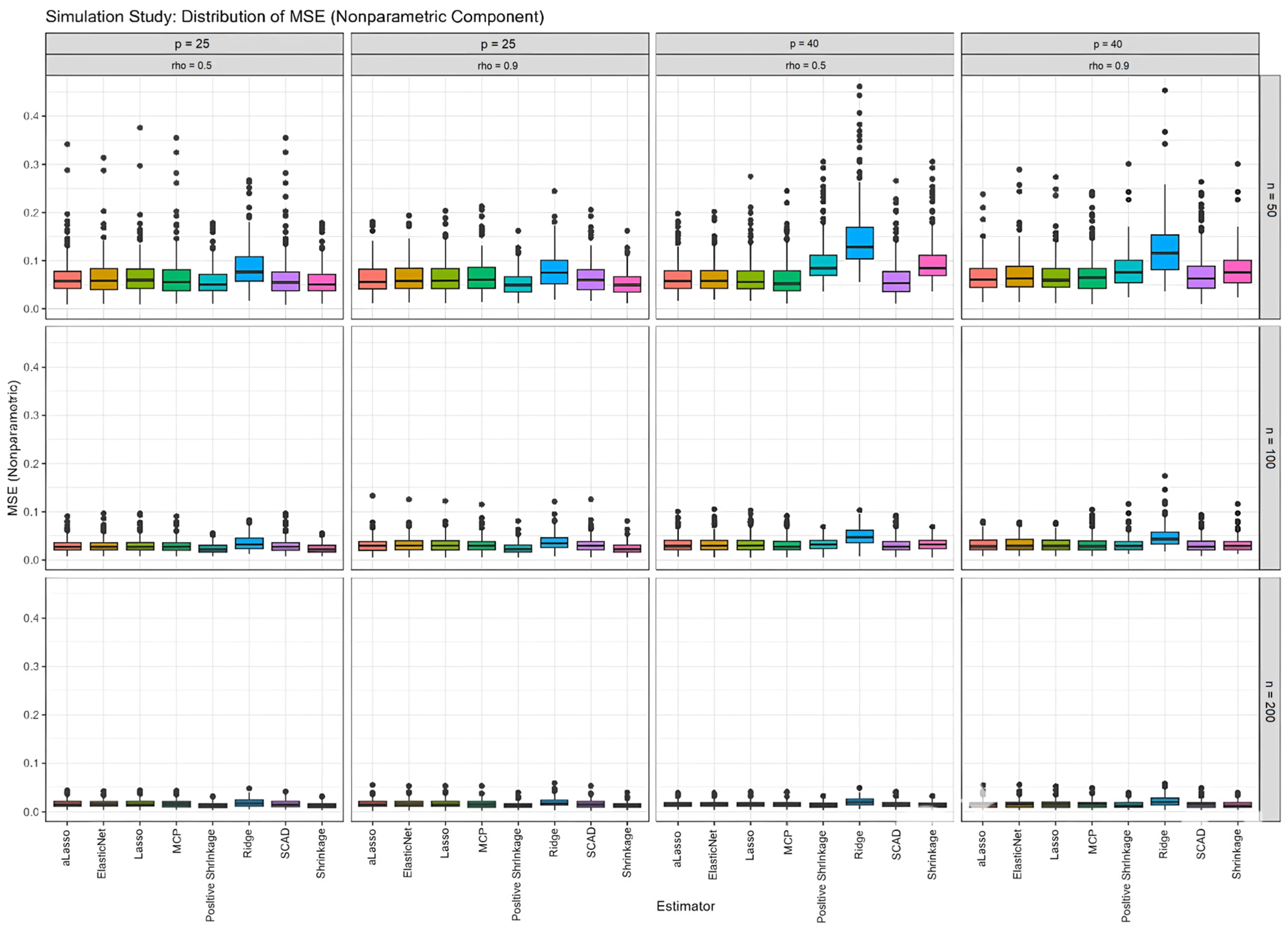
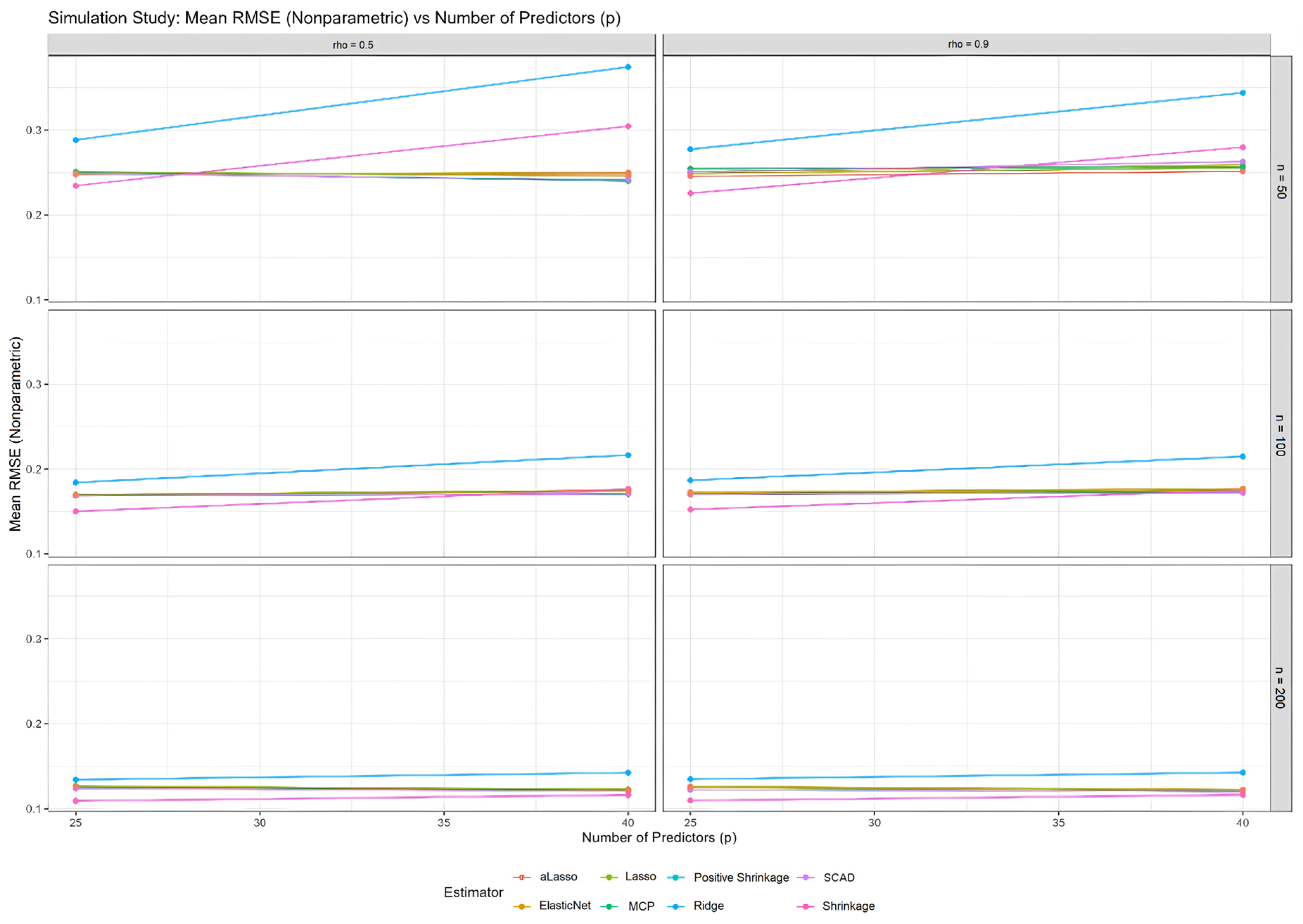
7.2. Analysis of the Nonparametric Component

This subsection examines the estimation of the nonparametric component of a semiparametric model, with the results shown in

Table 4. Simulation results of nonparametric component estimates for all simulation configurations.

	$\mathit{p}$	25						40
	$\mathit{\rho }$	0.5			0.9			0.5			0.9
$\mathit{n}$	Estimator	MSE	RMSE	RE	MSE	RMSE	RE	MSE	RMSE	RE	MSE	RMSE	RE
50	${\widehat{\mathbf{f}}}_{ENK}$	0.07	0.25	1.55	0.07	0.25	1.33	0.07	0.25	2.66	0.07	0.26	2.05
	${\widehat{\mathbf{f}}}_{LK}$	0.07	0.25	1.57	0.07	0.25	1.36	0.06	0.25	2.93	0.07	0.26	2.14
	${\widehat{\mathbf{f}}}_{MCK}$	0.07	0.25	1.63	0.07	0.25	1.34	0.06	0.24	3.31	0.07	0.26	2.32
	${\widehat{\mathbf{f}}}_{PS}$	0.06	0.23	1.51	0.05	0.23	1.51	0.10	0.30	1.51	0.08	0.28	1.51
	${\widehat{\mathbf{f}}}_{RK}$	0.09	0.29	1.00	0.08	0.28	1.00	0.15	0.37	1.00	0.12	0.34	1.00
	${\widehat{\mathbf{f}}}_{SK}$	0.07	0.25	1.68	0.07	0.25	1.39	0.06	0.24	3.34	0.08	0.26	2.24
	${\widehat{\mathbf{f}}}_S$	0.06	0.23	1.51	0.05	0.23	1.51	0.10	0.30	1.51	0.08	0.28	1.51
	${\widehat{\mathbf{f}}}_{aLK}$	0.07	0.25	1.54	0.06	0.25	1.40	0.07	0.25	2.79	0.07	0.25	2.18
100	${\widehat{\mathbf{f}}}_{ENK}$	0.03	0.17	1.24	0.03	0.17	1.24	0.03	0.18	1.74	0.03	0.18	1.59
	${\widehat{\mathbf{f}}}_{LK}$	0.03	0.17	1.26	0.03	0.17	1.28	0.03	0.17	1.82	0.03	0.18	1.65
	${\widehat{\mathbf{f}}}_{MCK}$ ${\widehat{\mathbf{f}}}_{PS}$	0.03	0.17	1.30	0.03	0.17	1.32	0.03	0.17	1.91	0.03	0.17	1.74
		0.02	0.15	1.50	0.02	0.15	1.50	0.03	0.18	1.50	0.03	0.18	1.50
	${\widehat{\mathbf{f}}}_{RK}$	0.04	0.18	1.00	0.04	0.19	1.00	0.05	0.22	1.00	0.05	0.21	1.00
	${\widehat{\mathbf{f}}}_{SK}$	0.03	0.17	1.30	0.03	0.17	1.31	0.03	0.17	1.89	0.03	0.17	1.76
	${\widehat{\mathbf{f}}}_S$	0.02	0.15	1.50	0.02	0.15	1.50	0.03	0.18	1.50	0.03	0.18	1.50
	${\widehat{\mathbf{f}}}_{aLK}$	0.03	0.17	1.25	0.03	0.17	1.28	0.03	0.17	1.79	0.03	0.18	1.63
200	${\widehat{\mathbf{f}}}_{ENK}$	0.02	0.13	1.17	0.02	0.13	1.18	0.02	0.12	1.43	0.02	0.12	1.41
	${\widehat{\mathbf{f}}}_{LK}$	0.02	0.13	1.18	0.02	0.12	1.22	0.02	0.12	1.44	0.02	0.12	1.44
	${\widehat{\mathbf{f}}}_{MCK}$ ${\widehat{\mathbf{f}}}_{PS}$	0.02	0.12	1.22	0.02	0.12	1.29	0.02	0.12	1.51	0.02	0.12	1.52
		0.01	0.11	1.50	0.01	0.11	1.50	0.01	0.12	1.50	0.01	0.12	1.50
	${\widehat{\mathbf{f}}}_{RK}$	0.02	0.13	1.00	0.02	0.13	1.00	0.02	0.14	1.00	0.02	0.14	1.00
	${\widehat{\mathbf{f}}}_{SK}$	0.02	0.12	1.23	0.02	0.12	1.29	0.02	0.12	1.52	0.02	0.12	1.52
	${\widehat{\mathbf{f}}}_S$	0.01	0.11	1.50	0.01	0.11	1.50	0.01	0.12	1.50	0.01	0.12	1.50
	${\widehat{\mathbf{f}}}_{aLK}$	0.02	0.13	1.18	0.02	0.12	1.20	0.02	0.12	1.46	0.02	0.12	1.43

for all simulations. Furthermore, the performance scores of the proposed methods are measured via the MSE and RMSE metrics. In addition, the estimated curves obtained from all methods are examined using all the distinct configurations in Figure 2 and Figure 3.

Table 4 presents the performance scores for the nonparametric component estimators in a similar format to Table 1, Table 2 and Table 3, which focuses on the parametric component. This table would quantify the accuracy and efficiency of each estimator in estimating the nonparametric function $f\left(t\right)$ under various simulation scenarios, varying sample size ($n$), number of predictors ($p$), and multicollinearity levels ($\rho$).

Based on the trends observed in Figure 2, Figure 3, Figure A1 and Figure A4, and the consistent findings in Table 1, Table 2 and Table 3, it is highly probable that Table 4 would further demonstrate the superior performance of ${\widehat{\mathbf{f}}}_{MCK}$, ${\widehat{\mathbf{f}}}_{SK}$, and the shrinkage estimators (${\widehat{\mathbf{f}}}_S$ and ${\widehat{\mathbf{f}}}_{PS}$), particularly in scenarios with high multicollinearity and smaller sample sizes. These estimators would likely exhibit lower MSE and RMSE values compared to others, indicating greater accuracy in estimating the nonparametric function and potentially higher RE values, suggesting greater efficiency relative to a reference estimator like ${\widehat{\mathbf{f}}}_{RK}$. The data in Table 4 provide the numerical backbone to support the visual observations in Figure 2 and the trends shown in Figure 3,Figure A1 and Figure A4, solidifying the conclusion that ${\widehat{\mathbf{f}}}_{MCK}$, ${\widehat{\mathbf{f}}}_{SK}$, ${\widehat{\mathbf{f}}}_S$, and ${\widehat{\mathbf{f}}}_{PS}$ offer significant advantages when estimating the nonparametric component of partially linear models.

Figure 2 provides a visual representation of how well each estimator captures the true nonparametric function, $f\left(t\right).$ When examining the fitted curves, especially under conditions of high multicollinearity ($\rho =0.9$) and small sample size ($n=50$), it becomes apparent that MCP (${\widehat{\mathbf{f}}}_{MCK}$), SCAD ${\widehat{\mathbf{f}}}_{SK}$, and the shrinkage estimators (${\widehat{\mathbf{f}}}_{PS} and {\widehat{\mathbf{f}}}_S$) produce curves that align more closely with the true function (represented by the black line) than those generated by Ridge (${\widehat{\mathbf{f}}}_{RK}$), Lasso (${\widehat{\mathbf{f}}}_{LK}$), aLasso (${\widehat{\mathbf{f}}}_{aLK}$), and ElasticNet (${\widehat{\mathbf{f}}}_{ENK}$). As the sample size increases, the differences become less visually striking, yet the advantage of ${\widehat{\mathbf{f}}}_{MCK}$, ${\widehat{\mathbf{f}}}_{SK}$, and shrinkage estimators persists, particularly when multicollinearity is present. This visual observation is consistent with the quantitative data shown in Figure 3, where these estimators consistently exhibit lower MSE values for the nonparametric component.

Figure 3 complements Figure 2 by quantifying the MSE of the nonparametric component against varying levels of multicollinearity. The trend observed mirrors that of Figure 1, i.e., MSE increases with multicollinearity for all estimators. However, ${\widehat{\mathbf{f}}}_{RK}$, consistently displays the highest MSE, while ${\widehat{\mathbf{f}}}_{MCK}$, ${\widehat{\mathbf{f}}}_{SK}$, and the shrinkage estimators maintain lower MSE values across the board. This quantitative evidence corroborates the visual findings of Figure 2, demonstrating that ${\widehat{\mathbf{f}}}_{MCK}$, ${\widehat{\mathbf{f}}}_{SK}$, and shrinkage estimators (${\widehat{\mathbf{f}}}_S$ and ${\widehat{\mathbf{f}}}_{PS}$,) provide more accurate estimates of the nonparametric function, especially when faced with correlated predictors. The relatively stable RMSE values of these better-performing estimators, even as the number of predictors increases, are shown in Figure A4 and further support their robustness in Appendix A.3.

8. Real Data

In this section, we implement our proposed six estimators, i.e., Ridge, Lasso, aLasso, SCAD, ElasticNet, and MCP, on real data. Our real data, Hitter’s dataset, can be obtained from the ISLR package in R. This dataset contains 322 rows and 20 variables. Three covariates, Division, League, and New League, which are not scalers, were deleted. The CN value obtained from this dataset is 5830, which indicates the presence of multicollinearity in the dataset. The remaining variables used for the estimation of a partially linear model are $\mathrm{S}\mathrm{a}\mathrm{l}\mathrm{a}\mathrm{r}\mathrm{y}$, $\mathrm{A}\mathrm{t}\mathrm{b}\mathrm{a}\mathrm{t}, \mathrm{R}\mathrm{u}\mathrm{n}\mathrm{s}, \mathrm{R}\mathrm{B}\mathrm{I}, \mathrm{W}\mathrm{a}\mathrm{l}\mathrm{k}\mathrm{s}, \mathrm{C}\mathrm{R}\mathrm{B}\mathrm{I}$, $\mathrm{C}\mathrm{w}\mathrm{a}\mathrm{l}\mathrm{k}\mathrm{s}$, $\mathrm{C}\mathrm{H}\mathrm{i}\mathrm{t}\mathrm{s}, \mathrm{C}\mathrm{H}\mathrm{m}\mathrm{r}\mathrm{u}\mathrm{n}$, $\mathrm{H}\mathrm{i}\mathrm{t}\mathrm{s}, \mathrm{H}\mathrm{m}\mathrm{r}\mathrm{u}\mathrm{n},$ $\mathrm{C}\mathrm{a}\mathrm{t}\mathrm{B}\mathrm{a}\mathrm{t}, \mathrm{C}\mathrm{r}\mathrm{u}\mathrm{n}\mathrm{s},$ and $\mathrm{P}\mathrm{u}\mathrm{t}\mathrm{s}\mathrm{O}\mathrm{u}\mathrm{t}\mathrm{s}$. In addition, the performance of the estimators is compared, and the results are shown in

Table 5. Overall model estimation performances of Hitter’s dataset based on introduced estimators.

Estimator	$\mathbf{RMSE} \widehat{\mathit{l}\mathit{o}\mathit{g}\left({\mathit{s}\mathit{a}\mathit{l}}_{\mathit{i}}\right)}$	$\mathbf{MSE} \mathit{l}\mathit{o}\mathit{g}\left({\mathit{s}\mathit{a}\mathit{l}}_{\mathit{i}}\right)$	$\mathbf{RE} \mathit{l}\mathit{o}\mathit{g}\left({\mathit{s}\mathit{a}\mathit{l}}_{\mathit{i}}\right)$
Ridge	0.577	0.333	1.000
Lasso	0.512	0.262	1.270
aLasso	0.443	0.196	1.697
SCAD	0.482	0.232	1.432
ElasticNet	0.474	0.224	1.484
MCP	0.482	0.232	1.432
Shrinkage	0.413	0.171	1.950
Pos. Shrinkage	0.405	0.164	2.025

and Figure 4 and Figure 5. Note that the logarithm of Salary is used as a response variable. From the visual inspection of the relationships between covariate and the response variable, the variable “$\mathrm{Y}\mathrm{e}\mathrm{a}\mathrm{r}\mathrm{s}$” has a significant nonlinear relationship with the response $\mathrm{l}\mathrm{o}\mathrm{g}\left(sal\right)$. The remaining 15 predictor variables are added to the parametric component of the model. Hence, the partially linear model can be written as follows:

$$log({sal}_i)={\mathbf{X}}_i^T\mathsf{\beta }+f({years}_i)+{\epsilon }_i,1\le i\le 263$$

(34)

where

$${\mathbf{X}}_i^T=\left[\begin{array}{c}{AtBat}_i, {Hits}_i, {HmRun}_i, {Runs}_i, {RBI}_i, {Walks}_i, {CAtBat}_i{, CHits}_i, {CHmRun}_i{CRuns}_i, \\ {CRBI}_i, {CWalks}_i, {PutOuts}_i, {Assists}_{ i}, {Errors}_i\end{array}\right]$$

Therefore, there is an $\left(263\times 15\right)$-dimensional covariate matrix for the parametric component of the model, and $\mathsf{\beta }={\left({\beta }_1,\dots ,{\beta }_{15}\right)}^T$ is the $\left(15\times 1\right)$-dimensional vector of the regression coefficients to be estimated.

Table 5 quantifies the performance of each estimator on the Hitters dataset using RMSE, MSE, and RE, all based on the prediction of log(Salary). The Shrinkage and Positive Shrinkage estimators stand out with the lowest RMSE and MSE values of 0.413 and 0.171, and 0.405 and 0.164, respectively. This indicates that these two methods provide the most accurate predictions for log(Salary) on this dataset. Their superior performance is further underscored by their RE values, 1.950 and 2.025, respectively, which demonstrate that they are almost twice as efficient as the Ridge estimator, which has an RE of 1.000 and performs the worst on this metric.

aLasso also performs well, with an RMSE of 0.443, MSE of 0.196, and RE of 1.697, outperforming Lasso, SCAD, ElasticNet, and MCP. Lasso, SCAD, ElasticNet, and MCP exhibit moderate performance, with RMSE values ranging from 0.474 to 0.512 and RE values between 1.270 and 1.484. These results are consistent with the simulation study, which suggested that shrinkage estimators, particularly positive shrinkage, and aLasso are effective in handling multicollinearity and achieving good prediction accuracy.

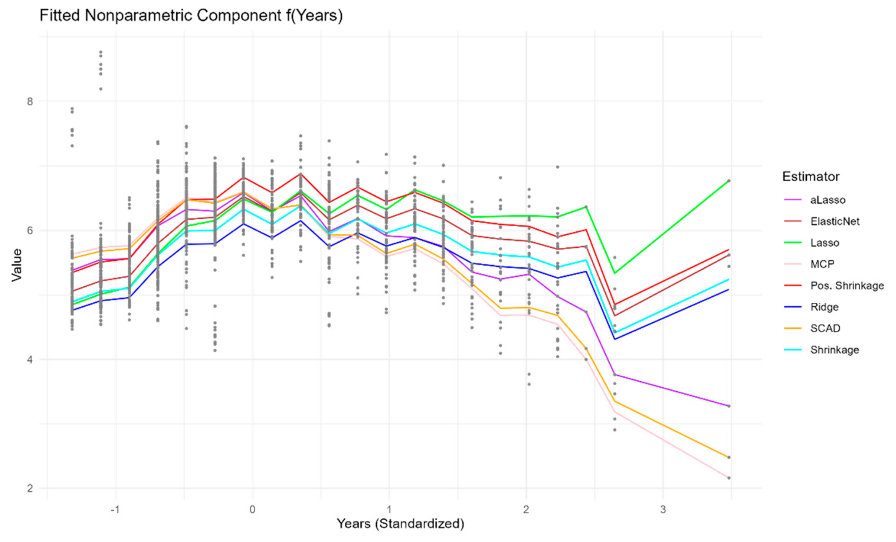
Figure 4 visually depicts the estimated nonparametric function f$\left(Years\right)$ for each estimator, revealing how they model the nonlinear relationship between a player’s standardized years of experience and their $log\left(Salary\right)$. The curves generally capture an initial increase in log(Salary) as years of experience increase, followed by a plateau or a slight decrease for players with more years. Notably, the curves produced by Ridge, MCP, and the shrinkage estimators are relatively similar and smooth, suggesting a consistent estimation of the underlying nonlinear trend. Lasso, aLasso, and ElasticNet exhibit some deviations from this trend, particularly in the middle range of the “Years” variable, indicating potential sensitivity to noise or specific data points. SCAD produces a curve that is very different from the others. The black dots, representing the observed data points adjusted for the parametric component’s effect, provide a visual reference for assessing the fit of each curve. The variation in the shapes of the curves highlights the influence of the chosen estimation method on the estimated nonparametric relationship, emphasizing the importance of considering different estimators and their potential impact on the interpretation of the results.

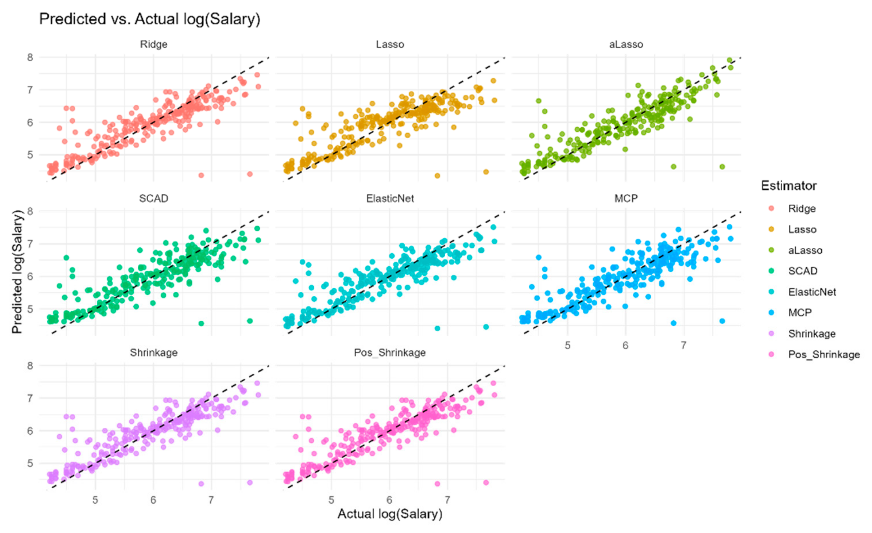
Figure 5 provides a visual comparison of the predicted log(Salary) values against the actual $log\left(Salary\right)$ values for each estimator, offering a direct assessment of their predictive accuracy. The points for Ridge, MCP, and the shrinkage estimators are more closely clustered around the diagonal line ($y=x$), indicating that their predictions are generally closer to the actual values. This observation aligns with the lower RMSE and MSE values reported for these estimators in Table 5. Conversely, Lasso, aLasso, and ElasticNet exhibit a wider spread of points around the diagonal, suggesting greater prediction errors and confirming their higher RMSE and MSE values in the table. The plot for SCAD has a different pattern that does not align with the diagonal. Overall, Figure 5 visually reinforces the quantitative findings in Table 5, demonstrating that Ridge, MCP, and particularly the shrinkage estimators achieve better predictive performance on the Hitters dataset, while Lasso, aLasso, and ElasticNet show relatively weaker performance. This visualization underscores the practical implications of estimator selection for achieving accurate predictions in partially linear models.

9. Conclusions

This paper focuses on the realm of semiparametric regression, specifically focusing on Partially Linear Regression Models (PLRMs) that incorporate both linear and nonlinear components. It considers a comprehensive review of six penalty estimation strategies: Ridge, Lasso, aLasso, SCAD, ElasticNet, and MCP. Recognizing the challenges posed by multicollinearity and the need for robust estimation in sparse models, we further introduce Stein-type shrinkage estimation techniques. The core of the study lies in evaluating the performance of these methods through both theoretical analysis and empirical investigation. A kernel smoothing technique, grounded in penalized least squares, is employed to estimate the semiparametric regression models.

The theoretical contributions include a partly asymptotic analysis of the proposed estimators, providing insights into their long-term behavior and robustness. The empirical investigation encompasses a simulation study that examines the estimators’ performance under various conditions, including different sample sizes, numbers of predictors, and levels of multicollinearity. Finally, the practical applicability of these methods is demonstrated through a real data example using the Hitters dataset, where the estimators are used to model baseball players’ salaries based on their performance metrics. The paper concludes that aLasso and shrinkage estimators exhibit superior performance in terms of prediction accuracy and efficiency in the presence of multicollinearity, especially the positive shrinkage, performing even better than aLasso.

In detail, the following points can be emphasized in terms of theoretical inferences, simulation and real data studies:

• The paper establishes the asymptotic properties of the proposed estimators, including Ridge, Lasso, aLasso, SCAD, ElasticNet, MCP, and the Stein-type shrinkage estimators, providing a theoretical foundation for their use in PLRMs.
• The theoretical results highlight the advantages of aLasso and shrinkage estimation, particularly in scenarios with high multicollinearity and sparsity.
• The simulation study demonstrates that aLasso and the shrinkage estimators, especially the positive shrinkage estimator, consistently outperform other methods in terms of lower Mean Squared Error (MSE) and Root Mean Squared Error (RMSE) for both the parametric and nonparametric components of the PLRM.
• The superior performance of aLasso and shrinkage estimators is more pronounced when the sample size is small and multicollinearity is high, confirming their robustness in challenging conditions.
• MCP and SCAD also exhibit strong performance in the simulations, often outperforming Ridge, Lasso, and ElasticNet, particularly when multicollinearity is present.
• The simulation results reveal that the choice of estimator can significantly impact the estimation of the nonparametric function, with aLasso and shrinkage estimators generally producing smoother and more accurate curves.
• The analysis of the Hitters dataset confirms the practical advantages of aLasso and shrinkage estimation, particularly positive shrinkage, in a real-world scenario with multicollinearity, as indicated by the high condition number.
• The shrinkage and aLasso estimators achieve the lowest RMSE and MSE values when predicting log(Salary), demonstrating their superior predictive accuracy compared to Ridge, Lasso, SCAD, ElasticNet, and MCP.
• The fitted nonparametric curves for the “Years” variable reveal interesting differences in how each estimator captures the nonlinear relationship between experience and salary, with aLasso and shrinkage estimators providing a balance between flexibility and smoothness.
• The real data results align with the findings of the simulation study, further supporting the use of aLasso and shrinkage estimation, especially positive shrinkage, in PLRMs when multicollinearity is a concern. Also, SCAD has unexpected results which needs more investigation.

While this study provides valuable theoretical and empirical insights into the performance of various penalty and shrinkage estimators for partially linear models, several limitations should be acknowledged. The simulation study uses a GCV for the bandwidth, which might not be the best choice. The analysis is also limited to a single real-world dataset (Hitters), and the simulation study, while comprehensive, does not cover all possible scenarios, such as different error distributions.

The computational cost of some estimators, particularly SCAD and MCP, is not explicitly addressed. Additionally, the choice of tuning parameters for the penalized estimators is obtained based on CV criterion, whereas in practice, these need to be carefully selected, potentially impacting the results. The paper’s theoretical results are based on regularity conditions that might not always hold in real-world applications. While shrinkage estimators are introduced and applied, a more in-depth investigation into their properties and performance would be beneficial. These limitations highlight the need for further research and careful consideration when applying these methods in practice.

References

- Engle, R.F.; Granger, C.W.; Rice, J.; Weiss, A. Semiparametric Estimates of the Relation Between Weather and Electricity Sales. J. Am. Stat. Assoc. 1986, 81, 310–320. [Google Scholar] [CrossRef]
- Green, P.J.; Silverman, B.W. Nonparametric Regression and Generalized Linear Models, 1st ed.; Chapman and Hall/CRC: London, UK, 1994. [Google Scholar]
- Ruppert, D.; Wand, M.P.; Carroll, R.J. Semiparametric Regression, 1st ed.; Cambridge University Press: Cambridge, UK, 2003. [Google Scholar]
- Speckman, P. Kernel Smoothing in Partial Linear Models. J. R. Stat. Soc. B 1988, 50, 413–436. [Google Scholar] [CrossRef]
- Heckman, N.E. Spline Smoothing in a Partly Linear Model. J. R. Stat. Soc. B 1986, 48, 244–248. [Google Scholar] [CrossRef]
- Tibshirani, R. Regression Shrinkage and Selection via the Lasso. J. R. Stat. Soc. B 1996, 58, 267–288. [Google Scholar] [CrossRef]
- Zou, H.; Zhang, H.H. On the Adaptive Elastic-Net with a Diverging Number of Parameters. Ann. Stat. 2009, 37, 1733–1751. [Google Scholar] [CrossRef]
- Ahmed, S.E. Penalty, Shrinkage and Pretest Strategies: Variable Selection and Estimation; Springer: New York, NY, USA, 2014. [Google Scholar]
- Wu, J.; Asar, Y. On Almost Unbiased Ridge Logistic Estimator for the Logistic Regression Model. Hacet. J. Math. Stat. 2016, 45, 989–998. [Google Scholar] [CrossRef]
- Ahmed, S.E.; Belaghi, R.A.; Hussein, A.; Safariyan, A. New and Efficient Estimators of Reliability Characteristics for a Family of Lifetime Distributions Under Progressive Censoring. Mathematics 2024, 12, 1599. [Google Scholar] [CrossRef]
- Ahmed, S.E.; Aydın, D.; Yılmaz, E. Penalty and Shrinkage Strategies Based on Local Polynomials for Right-Censored Partially Linear Regression. Entropy 2022, 24, 1833. [Google Scholar] [CrossRef]
- Yüzbaşı, B.; Arashi, M.; Ahmed, S.E. Big Data Analysis Using Shrinkage Strategies. arXiv 2017, arXiv:1704.05074. [Google Scholar]
- Yüzbaşı, B.; Ahmed, S.E.; Aydın, D. Ridge-Type Pretest and Shrinkage Estimations in Partially Linear Models. Stat. Pap. 2020, 61, 869–898. [Google Scholar] [CrossRef]
- Zou, H. The Adaptive Lasso and Its Oracle Properties. J. Am. Stat. Assoc. 2006, 101, 1418–1429. [Google Scholar] [CrossRef]
- Fan, J.; Li, R. Variable Selection via Nonconcave Penalized Likelihood and Its Oracle Properties. J. Am. Stat. Assoc. 2001, 96, 1348–1360. [Google Scholar] [CrossRef]
- Zhang, C.H. Nearly Unbiased Variable Selection under Minimax Concave Penalty. arXiv 2010, arXiv:1002.4734. [Google Scholar] [CrossRef] [PubMed]
- Aydın, D.; Ahmed, S.E.; Yılmaz, E. Right-Censored Time Series Modeling by Modified Semi-Parametric A-Spline Estimator. Entropy 2021, 23, 1586. [Google Scholar] [CrossRef]
- Yilmaz, E.; Yuzbasi, B.; Aydin, D. Choice of Smoothing Parameter for Kernel-Type Ridge Estimators in Semiparametric Regression Models. REVSTAT-Stat. J. 2021, 19, 47–69. [Google Scholar]
- Li, T.; Kang, X. Variable Selection of Higher-Order Partially Linear Spatial Autoregressive Model with a Diverging Number of Parameters. Stat. Pap. 2022, 63, 243–285. [Google Scholar] [CrossRef]
- Sun, L.; Zhou, X.; Guo, S. Marginal Regression Models with Time-Varying Coefficients for Recurrent Event Data. Stat. Med. 2011, 30, 2265–2277. [Google Scholar] [CrossRef]
- Sun, Z.; Cao, H.; Chen, L. Regression Analysis of Additive Hazards Model with Sparse Longitudinal Covariates. Lifetime Data Anal. 2022, 28, 263–281. [Google Scholar] [CrossRef]
- Hoerl, A.E.; Kennard, R.W. Ridge Regression: Biased Estimation for Nonorthogonal Problems. Technometrics 1970, 12, 55–67. [Google Scholar] [CrossRef]
- Yang, S.P.; Emura, T. A Bayesian Approach with Generalized Ridge Estimation for High-Dimensional Regression and Testing. Commun. Stat. Simul. Comput. 2017, 46, 6083–6105. [Google Scholar] [CrossRef]
- Bühlmann, P.; van de Geer, S. Statistics for High-Dimensional Data: Methods, Theory and Applications; Springer Science & Business Media: Heidelberg, Germany, 2011. [Google Scholar]
- Breheny, P.; Huang, J. Coordinate Descent Algorithms for Nonconvex Penalized Regression, with Applications to Biological Feature Selection. Ann. Appl. Stat. 2011, 5, 232–253. [Google Scholar] [CrossRef] [PubMed]
- Zou, H.; Hastie, T. Regularization and Variable Selection via the Elastic Net. J. R. Stat. Soc. B 2005, 67, 301–320. [Google Scholar] [CrossRef]
- Wang, L.; Liu, X.; Liang, H.; Carroll, R.J. Estimation and Variable Selection for Generalized Additive Partial Linear Models. Ann. Stat. 2013, 41, 712–741. [Google Scholar] [CrossRef]
- Ahmed, S.E.; Doksum, K.A.; Hossain, S.; You, J. Shrinkage, Pretest and Absolute Penalty Estimators in Partially Linear Models. Aust. N. Z. J. Stat. 2007, 49, 435–454. [Google Scholar] [CrossRef]
- Kubokawa, T. Highly-Efficient Quadratic Loss Estimation and Shrinkage to Minimize Mean Squared Error; Springer: Berlin/Heidelberg, Germany, 2020. [Google Scholar]
- Piladaeng, J.; Ahmed, S.E.; Lisawadi, S. Penalised, Post-Pretest, and Post-Shrinkage Strategies in Nonlinear Growth Models. Aust. N. Z. J. Stat. 2022, 64, 381–405. [Google Scholar] [CrossRef]
- Piladaeng, J.; Lisawadi, S.; Ahmed, S.E. Improving the performance of least squares estimator in a nonlinear regression model. In Proceedings of the Fourteenth International Conference on Management Science and Engineering Management, Chisinau, Moldova, 30 July–2 August 2020; Springer International Publishing: Berlin/Heidelberg, Germany, 2020; Volume 1, pp. 492–502. [Google Scholar]
- Ahmed, S.E.; Ahmed, F.; Yüzbaşı, B. Post-Shrinkage Strategies in Statistical and Machine Learning for High Dimensional Data, 1st ed.; Chapman and Hall/CRC: New York, NY, USA, 2023. [Google Scholar]
- Phukongtong, S.; Lisawadi, S.; Ahmed, S.E. Linear Shrinkage and Shrinkage Pretest Strategies in Partially Linear Models. E3S Web Conf. 2023, 409, 02009. [Google Scholar] [CrossRef]
- Li, D.; Racine, J. Nonparametric Econometrics: Theory and Practice. In Handbook of Research Methods and Applications in Empirical Macroeconomics; Edward Elgar Publishing: Northampton, MA, USA, 2013; pp. 3–28. [Google Scholar]
- Fan, J.; Gijbels, I. Local Polynomial Modelling and Its Applications: Monographs on Statistics and Applied Probability 66; CRC Press: Boca Raton, FL, USA, 1996. [Google Scholar]
- Zareamoghaddam, H.; Ahmed, S.E.; Provost, S.B. Shrinkage Estimation Applied to a Semi-Nonparametric Regression Model. Int. J. Biostat. 2020, 17, 23–38. [Google Scholar] [CrossRef]
- Ma, W.; Feng, Y.; Chen, K.; Ying, Z. Functional and Parametric Estimation in a Semi- and Nonparametric Model with Application to Mass-Spectrometry Data. Int. J. Biostat. 2013, 11, 285–303. [Google Scholar] [CrossRef]
- Asl, M.N.; Bevrani, H.; Belaghi, R.A.; Ahmed, S.E. Shrinkage and Sparse Estimation for High-Dimensional Linear Models. Adv. Intell. Syst. Comput. 2019, 1, 147–156. [Google Scholar]
- Aldeni, M.; Wagaman, J.C.; Amezziane, M.; Ahmed, S.E. Pretest and Shrinkage Estimators for Log-Normal Means. Comput. Stat. 2022, 38, 1555–1578. [Google Scholar] [CrossRef]
- Al-Momani, M.; Ahmed, S.E.; Hussein, A. Efficient Estimation Strategies for Spatial Moving Average Model. Adv. Intell. Syst. Comput. 2019, 1, 520–543. [Google Scholar]
- Reangsephet, O.; Lisawadi, S.; Ahmed, S.E. Post selection estimation and prediction in Poisson regression model. Thail. Stat. 2020, 18, 176–195. [Google Scholar]
- Reangsephet, O.; Lisawadi, S.; Ahmed, S.E. Weak signals in high-dimensional logistic regression models. In Proceedings of the Thirteenth International Conference on Management Science and Engineering Management, Ontario, ON, Canada, 5–8 August 2019; Springer International Publishing: Berlin/Heidelberg, Germany, 2020; Volume 1, pp. 121–133. [Google Scholar]
- Reangsephet, O.; Lisawadi, S.; Ahmed, S.E. A Comparison of Pretest, Stein-Type and Penalty Estimators in Logistic Regression Model. In Proceedings of the Eleventh International Conference on Management Science and Engineering Management, Kanazawa, Japan, 28–31 July 2017; Springer International Publishing: Berlin/Heidelberg, Germany, 2018; pp. 19–34. [Google Scholar]
- Shah, M.K.; Zahra, N.; Ahmed, S.E. On the Simultaneous Estimation of Weibull Reliability Functions. In Proceedings of the Thirteenth International Conference on Management Science and Engineering Management, Ontario, ON, Canada, 5–8 August 2019. [Google Scholar]
- Antoniadis, A.; Gijbels, I.; Verhasselt, A. Variable Selection in Additive Models Using P-Splines with Nonconcave Penalties. Ann. Inst. Stat. Math. 2012, 64, 5–27. [Google Scholar]
- Nadaraya, E.A. On Estimating Regression. Theory Probab. Appl. 1964, 9, 141–142. [Google Scholar] [CrossRef]
- Watson, G.S. Smooth Regression Analysis. Sankhyā A 1964, 26, 359–372. [Google Scholar]
- Yüzbaşı, B.; Ahmed, S.E.; Arashi, M.; Norouzirad, M. LAD, LASSO and Related Strategies in Regression Models. In Advances in Intelligent Systems and Computing; Springer: Berlin/Heidelberg, Germany, 2019. [Google Scholar]
- Staniswalis, J.G. The Kernel Estimate of a Regression Function in Likelihood-Based Models. J. Am. Stat. Assoc. 1989, 84, 276–283. [Google Scholar] [CrossRef]
- Frank, L.E.; Friedman, J.H. A Statistical View of Some Chemometrics Regression Tools. Technometrics 1993, 35, 109–135. [Google Scholar] [CrossRef]
- R Core Team. R: A Language and Environment for Statistical Computing; R Foundation for Statistical Computing: Vienna, Austria, 2015. [Google Scholar]
- Fu, W.; Knight, K. Asymptotics for Lasso-type estimators. Ann. Stat. 2000, 28, 1356–1378. [Google Scholar] [CrossRef]