A New Higher-Order Convergence Laplace–Fourier Method for Linear Neutral Delay Differential Equations

Abstract

In this article, a new higher-order convergence Laplace–Fourier method is developed to obtain the solutions of linear neutral delay differential equations. The proposed method provides more accurate solutions than the ones provided by the pure Laplace method and the original Laplace–Fourier method. We develop and show the crucial modifications of the Laplace–Fourier method. As with the original Laplace–Fourier method, the new method combines the Laplace transform method with Fourier series theory. All of the beneficial features from the original Laplace–Fourier method are retained. The solution still includes a component that accounts for the terms in the tail of the infinite series, allowing one to obtain more accurate solutions. The Laplace–Fourier method requires us to approximate the formula for the residues with an asymptotic expansion. This is essential to enable us to use the Fourier series results that enable us to account for the tail. The improvement is achieved by deriving a new asymptotic expansion which minimizes the error between the actual residues and those which are obtained from this asymptotic expansion. With both the pure Laplace and improved Laplace–Fourier methods, increasing the number of terms in the truncated series obviously increases the accuracy. However, with the pure Laplace method, this improvement is small. As we shall show, with the improved higher-order convergence Laplace–Fourier method, the improvement is significantly larger. We show that the convergence rate of the new Laplace–Fourier solution has a remarkable order of convergence. The validity of the new technique is corroborated by means of illustrative examples. Comparisons of the solutions of the new method with those generated by the pure Laplace method and the unmodified Laplace–Fourier approach are presented.

1. Introduction

Delay differential equations (DDEs) play an important role in many real-world processes [1,2,3,4,5,6,7]. Mathematical models based on different types of DDEs have been used to describe and study the dynamics of many infectious diseases [3,8,9,10,11,12,13,14,15]. Also, real-world applications of DDEs appear in a variety of fields such as physics, epidemiology, and engineering [2,7,16,17]. For example, NDDEs appear when modeling electrical circuits that include delayed elements [18]. Interestingly, DDEs have been used in climate models related to El Niño–Southern Oscillation (ENSO) [19]. In [20], an NDDE appears in the Partial Element Equivalent Circuit formulation of Maxwell’s equations. In [21], an NDDE was used to model the stick–slip problem related to the torsional motion of the drill. Finally, in [22], a linear NDDE was used for a budget constraint related to physical capital in an economic model. Thus, we can see that there are a variety of applications of NDDEs to real world problems.

The complexity of DDEs is usually greater than those of ordinary differential equations (ODEs). The delays can cause a stable equilibrium to become unstable, and periodic solutions can arise [10,23,24,25,26,27,28]. Recently, there has been an increasing interest in the development of methods for finding and studying the solutions of a variety of DDEs, including some of fractional order [29,30,31,32,33,34,35,36]. The classical method for solving DDEs is the method of steps (MoS), which generates an analytical piecewise solution. This method is based on a stepwise process that requires solving a differential equation in different time intervals [7,37,38,39,40]. However, for many DDEs, the MoS encounters the phenomenon of expression swell [37,40,41]. Thus, for many DDEs the MoS is not able to generate the solution for the whole time domain. However, in some cases the MoS can be used to find a closed-form solution [37,40,41].

There are numerous classifications for the DDEs, amongst which one important type is represented by the neutral delay differential equations (NDDEs). In these equations, the time delays appear in the state variable derivative [42,43,44,45,46,47,48,49,50]. NDDEs arise in numerous mathematical models involving problems in engineering and science [51,52,53,54]. NDDEs have been solved by a variety of methods [33,47,55,56].

The main aim of this paper is to present a new higher-order convergence Laplace–Fourier method, which produces an essentially analytical solution that significantly reduces the error. The Laplace–Fourier method is based on the combination of the Laplace transform and Fourier series theory and can be used to obtain the solutions of linear NDDEs [57]. The solution is composed of a closed-form part and an infinite series [57]. The method requires computing the poles of the Laplace transform equation and computing the residues by Cauchy’s residue theorem. For the closed-form part however, one must use an approximate formula for the location of the poles. In this paper, a new formula developed by the authors provides an improved approximate for the location of the poles. More importantly, however, an improved formula for approximating the residues at the poles is also derived. This new formula is then used to show that the new higher-order convergence Laplace–Fourier method is significantly more accurate than the original Laplace–Fourier method. To the best of our knowledge, there is no similar method close to the one developed in this work besides the regular Laplace–Fourier method developed by the same authors [57]. There are a variety of methods to obtain numerical solutions, and some mathematical software have implemented them [58,59]. For instance, Matlab has the built-in function dde23, which generates numerical solutions for DDEs. It has been shown that analytical solutions developed using Laplace and Laplace–Fourier methods are oftentimes more accurate than the numerical ones [41,57,60].

The pure Laplace method has been used recently to solve fractional linear DDEs [61]. In [62], the Laplace method was applied to solve systems of linear retarded and neutral delay differential equations. It was found that in some cases the solution asymptotically approaches a limit cycle. In [57], it was shown that a previous Laplace–Fourier method can improve the accuracy of the solution of linear DDEs. The Laplace–Fourier method improves the pure Laplace method by taking into account the contribution of all the terms in the pure Laplace solution (infinite series) for terms such that $N>k$. This is accomplished by approximating the tail of the infinite series with a harmonic Fourier series. Then, in turn, one determines an analytic formula for the series. This formula, which constitutes an important component of the solution, is a piecewise continuous function that is composed of polynomials. The Laplace–Fourier method has the versatility to modify the degree of polynomials in order to improve the accuracy. The Laplace–Fourier method also requires us to approximate the formula for the residues with an asymptotic expansion. This is essential to enable us to proceed and use the Fourier series results for solving linear NDDEs.

2. Definitions for NDDEs and Laplace Transform

To facilitate the introduction of the new Laplace–Fourier method, we will recap some of the basic foundations (for more details, see [41,57]). Let us focus on the subclass of NDDEs of the following form:

$$y^{\prime }\left(t\right)=ay\left(t\right)+b{y}^{\prime }(t-\tau )+cy(t-\tau ),t>0,b\ne 0.$$

(1)

For the history function $y\left(t\right)=H\left(t\right)$, $t\in [-\tau ,0]$. The history function can be seen as an initial condition. There are many admissible classes of history functions, and they play a role in the computation of the the solution (see [53,57,63,64] for more details). For instance, history functions can be polynomials or trigonometric functions [41,57]. We will see that, depending on the history function, we can obtain a variety of solutions.

2.1. Applying of the Laplace Transform

Taking the Laplace transform of Equation (1) and solving for $Y\left(s\right)$, one obtains

$$Y\left(s\right)={\displaystyle \frac{N\left(s\right)}{s-a-(bs+c)e^{-s\tau }}},$$

(2)

where $N\left(s\right)=H\left(0\right)-bH(-\tau )+(bs+c)e^{-s\tau }{\int }_{-\tau }^{0}H\left(v\right)e^{-sv}dv$. Assuming that any singularities resulting from the integral term in $N\left(s\right)$ are removable, the relevant poles are determined by the roots of the equation

$$D\left(s\right)=s-a-(bs+c)e^{-s\tau }=0.$$

(3)

Note that $N\left(s\right)$ and $D\left(s\right)$ might have (very unlikely due to the four parameters $a,b,c$, and $\tau$) zeroes in common. In this case, these singularities are removable [41,60,62]. Regardless of the zeroes in common, the Laplace–Fourier method can generate the solution by using the Cauchy residue theorem [41,57]. The exact number of real roots can be at most three, and this depends on the parameters $a,b,c$, and the time delay $\tau$. It can be shown that the real roots of the denominator $D\left(s\right)$ are given by the intersection of the Lambert function and a linear function. Thus, we can have at most three real roots. In the case of no real poles, the Laplace–Fourier solution would be given only in terms of the complex poles. It is important to remark that for the piecewise polynomial component of the higher-order convergence Laplace–Fourier solution, only the complex poles play a role.

2.2. Complex Poles

Dividing the characteristic Equation (3) by s reveals that the approximate location of the poles (for $\left|s\right|$ large and $\mathfrak{Im}\left(s\right)>0$) is given by

$$s_k={\displaystyle \frac{ln\left(b\right)+2k\pi i}{\tau }},k\in \mathbb{N},$$

(4)

when $b>0$. For $b<0$, we have a different formula, but it is similar to that in [41]. These formulas can be used as the initial guesses for determining the actual poles by some numerical method to find zeroes, such as Newton’s method (details in [41]). Applying the inverse Laplace transform to Equation (2) and Cauchy’s residue theorem, one can obtain the solution $y\left(t\right)$ of the NDDE (1). However, this requires finding the residues at the infinitely many poles. Applying L’Hopital’s rule, one obtains that the related residues at the poles are given by

$$c_k={\displaystyle \frac{N\left(r_k\right)}{1+(b{r}_k\tau -b+c\tau )e^{-r_k\tau }}},$$

(5)

where $r_k,k\in \mathbb{N}$ are the sequence of complex poles above the imaginary axis. In order to distinguish the actual poles from the approximates given by Equation (4), we shall use $r_k$. Once the poles have been determined, we can use the Cauchy residue theorem to determine $y\left(t\right)$. Without loss of generality and assuming that there is one real root ($r_0$), then we can write the solution as

$$y\left(t\right)=c_0{e}^{r_{0}t}+2\sum _{k=1}^{\infty }\mathfrak{Re}\left(c_k{e}^{r_{k}t}\right).$$

(6)

Thus, regardless of the number of real roots (at most three), we can always obtain a solution in terms of an infinite non-harmonic series for the linear DDE (1) if $H\left(t\right)\in C^{\infty }$. In [41], it has been shown that any singularities resulting from the integral term in $N\left(s\right)$ are removable, and all of the relevant poles are determined by the roots of the equation $D\left(s\right)=0$. Moreover, the solution is unique (see [63,64]). The solution of the NDDE (1) at some point would have a discontinuous derivative [64]. The smoothing property is not valid for NDDEs, and the solution $y\left(t\right)$ is always as smooth as the history function $H\left(t\right)$ (see [64]). For instance, if the history function $H\left(t\right)$ is discontinuous at some point $t=t_0$, then the exact solution of the NDDE (1) would be discontinuous at $t=t_0+\tau$ [65,66].

2.3. Laplace–Fourier Solution

The main shortcoming of the pure Laplace transform method, when utilized for solving DDEs, is the slow convergence rate of the series solution in the vicinity of the points $t=m\tau ,m\in \mathbb{N}$ [41]. The Laplace–Fourier is able to improve the convergence rate without increasing the number of terms in the series [57]. For the Laplace–Fourier method, we shall assume that $H\left(t\right)\in C^{\infty }$ in order to be able to guarantee the existence of the Laplace–Fourier solution. Recall that the approximate locations of the poles (for $\left|s\right|$ large, $b>0$, and $\mathfrak{Im}\left(s\right)>0$) are given by Equation (4). Therefore, the tail of the series (for $k\ge N$) can be approximated by

$$y_a\left(t\right)\simeq 2\sum _{k=N}^{\infty }\mathfrak{Re}\left(c_k{e}^{\left[{\displaystyle \frac{ln\left(b\right)+2k\pi i}{\tau }}\right]t}\right)\simeq 2e^{{\displaystyle \frac{ln\left(b\right)}{\tau }}t}\sum _{k=N}^{\infty }\mathfrak{Re}\left(c_k{e}^{{\displaystyle \frac{2k\pi i}{\tau }}t}\right).$$

(7)

Observe that being able to remove the $ln\left(b\right)$ term from inside of the sum leaves one with a regular, harmonic Fourier series (inside the sum). Note that a more accurate location of the poles that includes the parameters a and b would not allow us to write the approximated solution $y_a\left(t\right)$ in terms of a regular, harmonic Fourier series. Thus, it is imperative that one uses Equation (4) for the Laplace–Fourier method [57]. However, the actual complex poles depend on $a,b,c$, and $\tau$. Indeed, in Section 4, a more accurate formula for the location of the poles is presented. It can be shown (we will verify this later in Section 3) that the asymptotic expansion for the $c_k$’s at $k=\infty$ is (typically) of the form

$$c_k^a\simeq {\displaystyle \frac{a_2}{{\left(\frac{2k\pi i}{\tau }\right)}^2}}+{\displaystyle \frac{a_3}{{\left(\frac{2k\pi i}{\tau }\right)}^3}}+\cdots ,$$

(8)

in which all the coefficients $a_m$ are real. Hence, labeling ${\alpha }_k={\displaystyle \frac{2k\pi }{\tau }}$, one obtains

$$y_a\left(t\right)\simeq 2e^{{\displaystyle \frac{ln\left(b\right)}{\tau }}t}\sum _{k=N}^{\infty }\mathfrak{Re}\left(\left[{\displaystyle \frac{-a_2}{{\alpha }_k^2}}+{\displaystyle \frac{i{a}_3}{{\alpha }_k^3}}+\cdots \right]e^{{\alpha }_{k}it}\right),$$

(9)

or using Euler’s formula, one obtains

$$y_a\left(t\right)\simeq 2e^{{\displaystyle \frac{ln\left(b\right)}{\tau }}t}\sum _{k=N}^{\infty }\left[{\displaystyle \frac{-a_2}{{\alpha }_k^2}}cos\left({\alpha }_{k}t\right)-{\displaystyle \frac{a_3}{{\alpha }_k^3}}sin\left({\alpha }_{k}t\right)+\cdots \right].$$

(10)

which can then be rewritten as

$$\begin{array}{ccc}{y}_a\left(t\right)\hfill & \simeq \hfill & 2e^{{\displaystyle \frac{ln\left(b\right)}{\tau }}t}{\displaystyle \sum _{k=1}^{\infty }}\left[{\displaystyle \frac{-a_2}{{\alpha }_k^2}}cos\left({\alpha }_{k}t\right)-{\displaystyle \frac{a_3}{{\alpha }_k^3}}sin\left({\alpha }_{k}t\right)+\cdots \right]\hfill \\ \hfill & \hfill & \\ \hfill & \hfill & -2e^{{\displaystyle \frac{ln\left(b\right)}{\tau }}t}{\displaystyle \sum _{k=1}^{N-1}}\left[{\displaystyle \frac{-a_2}{{\alpha }_k^2}}cos\left({\alpha }_{k}t\right)-{\displaystyle \frac{a_3}{{\alpha }_k^3}}sin\left({\alpha }_{k}t\right)+\cdots \right].\hfill \end{array}$$

(11)

Observe that the infinite series in the sum which starts at $k=1$ is, by design, an exact match with the classical type harmonic Fourier Series [67,68]. Therefore, using the relevant Fourier series formulas, enables us to replace this sum with a closed-form analytic expression in the form of a piecewise continuous function.

2.4. Fourier Series Results

The results of the previous section were obtained by assuming that $b>0$, where the approximate location of the poles is given by Equation (4). For the sake of clarity, let us retain this assumption in this section. For the case where $b<0$, the formulas are similar and can be found in [57]. Some of the following results can also be found in [57]. However, we include them here for self-readability.

On the interval $0<x<\tau$, with ${\alpha }_n={\displaystyle \frac{2n\pi }{\tau }}$, we have that

$$\sum _{n=1}^{\infty }{\displaystyle \frac{{cos(\alpha }_{n}x)}{{\alpha }_n^2}}={\displaystyle \frac{3x^2-3x\tau +{\tau }^2/2}{12}}=p_2\left(x\right).$$

(12)

Subsequent results for polynomials of higher degree may be obtained via integration [57,68]. For example,

$$\sum _{n=1}^{\infty }{\displaystyle \frac{sin{(\alpha }_{n}x)}{{\alpha }_n^3}}={\displaystyle \frac{x(x-\tau /2)(x-\tau )}{12}}=p_3\left(x\right),$$

(13)

and

$$\sum _{n=1}^{\infty }{\displaystyle \frac{cos{(\alpha }_{n}x)}{{\alpha }_n^4}}={\displaystyle \frac{{\tau }^4}{1440}}-{\displaystyle \frac{x^2{(x-\tau )}^2}{48}}=p_4\left(x\right).$$

(14)

Therefore using these polynomials enables one to rewrite $y_a\left(t\right)$ as

$$\begin{array}{cc}\hfill y_a\left(t\right)& \simeq 2e^{{\displaystyle \frac{ln\left(b\right)}{\tau }}t}\left[-a_2{p}_2\left(t\right)-a_3{p}_3\left(t\right)+a_4{p}_4\left(t\right)\right]\hfill \\ \hfill & -2e^{{\displaystyle \frac{ln\left(b\right)}{\tau }}t}\sum _{k=1}^{N-1}\left[{\displaystyle \frac{-a_2}{{\alpha }_k^2}}cos\left({\alpha }_{k}t\right)-{\displaystyle \frac{a_3}{{\alpha }_k^3}}sin\left({\alpha }_{k}t\right)+{\displaystyle \frac{a_4}{{\alpha }_k^4}}cos\left({\alpha }_{k}t\right)\right],0<t<\tau .\hfill \end{array}$$

(15)

Therefore,

$$\begin{array}{cc}\hfill y_a\left(t\right)& \simeq 2e^{{\displaystyle \frac{ln\left(b\right)}{\tau }}t}{P}_e\left(t\right)\hfill \\ \hfill & -2e^{{\displaystyle \frac{ln\left(b\right)}{\tau }}t}\sum _{k=1}^{N-1}\left[{\displaystyle \frac{-a_2}{{\alpha }_k^2}}cos\left({\alpha }_{k}t\right)-{\displaystyle \frac{a_3}{{\alpha }_k^3}}sin\left({\alpha }_{k}t\right)+{\displaystyle \frac{a_4}{{\alpha }_k^4}}cos\left({\alpha }_{k}t\right)\right],0<t<\infty .\hfill \end{array}$$

(16)

where $P_e\left(t\right)$ is the $\tau$-periodic extension of the relevant polynomial on the basic interval: $0<t<\tau$. Then, combining the above formula with Equation (6), one obtains

$$y\left(t\right)\simeq c_0{e}^{r_{0}t}+2e^{{\displaystyle \frac{ln\left(b\right)}{\tau }}t}{P}_e\left(t\right)+2\sum _{k=1}^N\mathfrak{Re}\left(c_k{e}^{r_{k}t}-c_k^a{e}^{\left[{\displaystyle \frac{ln\left(b\right)+2k\pi i}{\tau }}\right]t}\right).$$

(17)

in which $c_k^a$ is given by Equation (8). We also note that it is possible to extend Equation (17) by including polynomials of higher degrees.

2.5. Further Insight into the Laplace–Fourier Method

The pure truncated Laplace solution does not include the contribution of all the terms. The most novel aspect of the Laplace Fourier solution is that it does account for these excluded terms [57]. The Laplace–Fourier method is very accurate in the case where $ab+c=0$. This is due to the fact that the estimates (4) provide an exact formula for the poles, since one obtains

$$D\left(s_k\right)=s_k-a-\left(b{s}_k+c\right)e^{-\left({\displaystyle \frac{ln\left(b\right)+2k\pi i}{\tau }}\right)\tau }=s_k-a-{\displaystyle \frac{1}{b}}(b{s}_k+c)=-\left(a+{\displaystyle \frac{c}{b}}\right).$$

(18)

Thus, Equation (17) becomes

$$y\left(t\right)\simeq c_0{e}^{r_{0}t}+2e^{{\displaystyle \frac{ln\left(b\right)}{\tau }}t}{P}_e\left(t\right)+2e^{{\displaystyle \frac{ln\left(b\right)}{\tau }}t}\sum _{k=1}^N\mathfrak{Re}\left([c_k-c_k^a]e^{{\displaystyle \frac{2k\pi i}{\tau }}t}\right)$$

(19)

Then, the series has an improved convergence rate, for the Nth partial sum, of the order $O\left({\displaystyle \sum _{k=N+1}^{\infty }}{k}^{-5}\right)=O\left(N^{-4}\right)$ [57]. This specific convergence rate assumes that the polynomials in $P_e\left(t\right)$ are of order four. The convergence rate can be further enhanced by including additional polynomials of higher orders.

3. New Higher-Order Convergence Laplace–Fourier Method

For the solution of the NDDE (1), one obtains that the portion of $y\left(t\right)$ related to these complex poles is given by

$$y\left(t\right)=2\sum _{k=1}^{\infty }\mathfrak{Re}\left(c_k{e}^{r_{k}t}\right),$$

(20)

in which we recall that

$$c_k\left(s\right)={\displaystyle \frac{H\left(0\right)-bH(-\tau )+(c+bs)e^{-s\tau }{\int }_{-\tau }^{0}H\left(v\right)e^{-sv}dv}{1+(bs\tau -b+c\tau )e^{-s\tau }}}.$$

(21)

However, we also know that at each of the poles $D\left(s\right)$. In which case,

$$e^{-s\tau }={\displaystyle \frac{s-a}{bs+c}}.$$

(22)

Thus, this enables us to rewrite the denominator in Equation (21) as

$$D^{\prime }\left(s\right)=1+(bs\tau -b+c\tau ){\displaystyle \frac{s-a}{bs+c}},$$

(23)

providing $s\in \left\{r_k,k\in \mathbb{N}\right\}=W$. Now applying integration by parts to the integral in the numerator of Equation (21), we find that

$${\int }_{-\tau }^{0}H\left(v\right)e^{-sv}dv={\displaystyle \frac{H(-\tau )e^{s\tau }-H\left(0\right)}{s}}+{\displaystyle \frac{H^{\prime }(-\tau )e^{s\tau }-H^{\prime }\left(0\right)}{s^2}}+O\left(s^{-3}\right).$$

(24)

Substituting the above expression into the numerator in Equation (21) and using Equation (22) to replace all of the exponential terms, it can be shown that

$$N\left(s\right)={\displaystyle \frac{1}{s}}\left[cH(-\tau )+aH\left(0\right)+b{H}^{\prime }(-\tau )-H^{\prime }\left(0\right)\right]+O\left(s^{-2}\right),s\in W.$$

(25)

Therefore,

$$\underset{s\to \infty }{lim}{\displaystyle \frac{N\left(s\right)}{D^{\prime }\left(s\right)}}={\displaystyle \frac{1}{\tau s^2}}\left[cH(-\tau )+aH\left(0\right)+b{H}^{\prime }(-\tau )-H^{\prime }\left(0\right)\right]+O\left(s^{-3}\right),s\in W.$$

(26)

Recall, however, that the Fourier series results that are used require an asymptotic expansion with respect to the frequencies as $k\to \infty$. Therefore, substituting $s_k=ln\left(b\right)/\tau +i{\alpha }_k$ into the above equation, one obtains

$$c_k^a=\underset{k\to \infty }{lim}{\displaystyle \frac{N\left(s_k\right)}{D^{\prime }\left(s_k\right)}}={\displaystyle \frac{-a_2}{{\alpha }_k^2}}+i{\displaystyle \frac{a_3}{{\alpha }_k^3}}+O\left({\alpha }_k^{-4}\right).$$

(27)

where

$$a_2={\displaystyle \frac{1}{\tau }}\left[cH(-\tau )+aH\left(0\right)+b{H}^{\prime }(-\tau )-H^{\prime }\left(0\right)\right]$$

(28)

The analytic expressions for the subsequent coefficients ($a_n$) become progressively more complicated. They can, however, be easily found using the series command with Maple software (https://www.maplesoft.com/products/maple/).

The original Laplace–Fourier method uses the Formula (4) for the poles $s_k$ and substitutes them into Equation (21) right at the outset. As a consequence, all of the exponential terms simplify to

$$e^{-s_k\tau }=e^{-(ln\left(b\right)/\tau +i{\alpha }_k)\tau }={\displaystyle \frac{1}{b}},\forall k.$$

(29)

With, as we observe, a zero imaginary part. Therefore, the term

$$s_k{e}^{-s_k\tau }={\displaystyle \frac{1}{b}}\left({\displaystyle \frac{ln\left(b\right)+2k\pi i}{\tau }}\right)$$

(30)

However, the actual/exact pole $r_k$ is only relatively close to $s_k$. Therefore, the term $e^{-r_k\tau }$ has a relatively small non-zero imaginary part. Let us denote this imaginary part as ${ϵ}_{k}i$. Then, the formula for ${ϵ}_k$ can be derived via the asymptotic expansion for ${\displaystyle \frac{s-a}{bs+c}},$ which is given by ${\displaystyle \frac{1}{b}}(1-(a+c/b)s^{-1}+O\left(s^{-2}\right))$. Thus, when multiplied by $r_k$, one obtains

$$r_k{e}^{-r_k\tau }={\displaystyle \frac{1}{b}}\left({\displaystyle \frac{ln\left(b\right)+2k\pi i}{\tau }}-(a+c/b)\right)+O\left(k^{-1}\right),$$

(31)

for large k. Notice that this $s{e}^{-s\tau }$ term appears in both the numerator and the denominator of Equation (21). Therefore, the expansion of $c_k$ in the original Laplace–Fourier method is only exact when $ab+c=0$. However, when the contribution from the $a+c/b$ term is significant, the original Laplace–Fourier method is oftentimes only marginally better than the pure Laplace solution, and in some extreme cases, might be less accurate. In this paper, we have developed a new higher-order convergence Laplace–Fourier method that addresses this shortcoming. In the next section, we will analyze the convergence of the new Laplace–Fourier method.

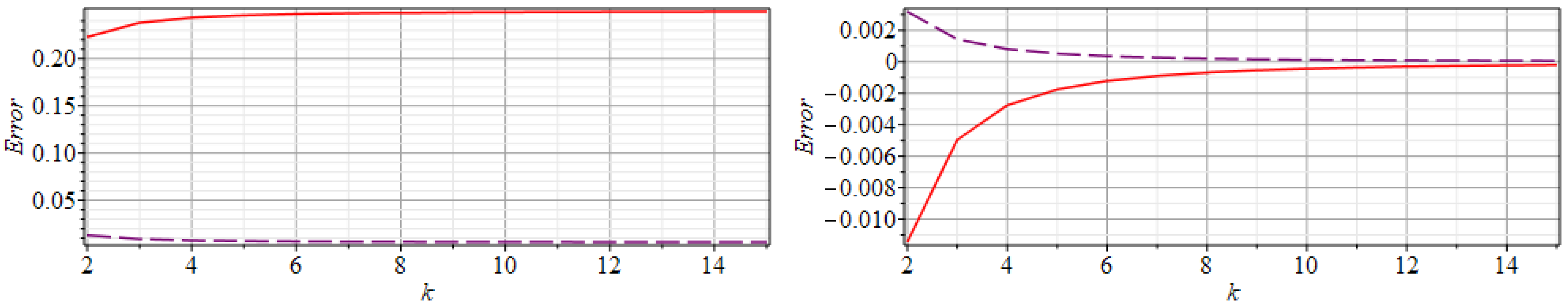
4. Convergence Rate of the New Higher-Order Convergence Laplace–Fourier Solution

In order to establish the convergence rate of the series in Equation (17), we shall need an improved approximate for the location of the poles for large k. This can be obtained by assuming that $s_k$ is of the form

$$s_k={\displaystyle \frac{ln\left(b\right)+2k\pi i}{\tau }}+{\displaystyle \frac{\beta }{k^2}}+i{\displaystyle \frac{\gamma }{k}},k\in \mathbb{N}$$

(32)

The constants $\beta$ and $\gamma$, which depend on all the parameters $a,b,c$, and $\tau$, can be determined by substituting Equation (32) into Equation (22). Then, we equate the coefficients in the respective asymptotic expansions for large k. For the term on the left, it can be shown that

$$e^{-s_k\tau }={\displaystyle \frac{1}{b}}{e}^{-({\displaystyle \frac{\beta }{k^2}}+i{\displaystyle \frac{\gamma }{k}})\tau }={\displaystyle \frac{1}{b}}-i{\displaystyle \frac{\gamma \tau }{bk}}-{\displaystyle \frac{\beta \tau +\frac{1}{2}{\gamma }^2{\tau }^2}{b{k}^2}}+O\left(k^{-3}\right)$$

(33)

and for the term on the right-hand side of Equation (22), one obtains

$${\displaystyle \frac{s_k-a}{b{s}_k+c}}={\displaystyle \frac{1}{b}}+i{\displaystyle \frac{\left(ab+c\right)\tau }{2b^2\pi k}}-{\displaystyle \frac{\tau (ab+c)(bln(b)+c\tau )}{4b^3{\pi }^2{k}^2}}+O\left(k^{-3}\right).$$

(34)

Then, equating the relevant coefficients, one obtains the following system of equations

$$-{\displaystyle \frac{\gamma \tau }{b}}={\displaystyle \frac{\left(ab+c\right)\tau }{2b^2\pi }}$$

(35)

and

$${\displaystyle \frac{\beta \tau +\frac{1}{2}{\gamma }^2{\tau }^2}{b}}={\displaystyle \frac{\tau (ab+c)(bln(b)+c\tau )}{4b^3{\pi }^2}}.$$

(36)

Solving this system for $\beta$ and $\gamma$, we find that

$$\beta ={\displaystyle \frac{(ab+c)(2bln(b)-\tau (ab-c\left)\right)}{8b^2{\pi }^2}},$$

(37)

and

$$\gamma ={\displaystyle \frac{-\left(ab+c\right)}{2b\pi }}.$$

(38)

Remark 1.

This improved approximate $s_k$, which also accounts for the contributions from the parameters a and c, can also be used as a more accurate initial guess in the subroutine where one computes the actual poles $r_k$.

These results can now be used to verify that the convergence rate of the new improved Laplace–Fourier solution is $O\left(N^{-3}\right)$. In order to accomplish this, let us recall Equation (17):

$$y\left(t\right)\simeq c_0{e}^{r_{0}t}+2e^{{\displaystyle \frac{ln\left(b\right)}{\tau }}t}{P}_e\left(t\right)+2\sum _{k=1}^N\mathfrak{Re}\left(c_k{e}^{r_{k}t}-c_k^a{e}^{\left[{\displaystyle \frac{ln\left(b\right)+2k\pi i}{\tau }}\right]t}\right)$$

(39)

and focus on the residues in the sum. Now, we know from Equation (26) that, for large s

$$c_k\left(s\right)={\displaystyle \frac{b_2}{s^2}}+{\displaystyle \frac{b_3}{s^3}}+{\displaystyle \frac{b_4}{s^4}}+O\left(s^{-5}\right),s\in W,$$

(40)

in which

$$b_2={\displaystyle \frac{1}{\tau }}\left[cH(-\tau )+aH\left(0\right)+b{H}^{\prime }(-\tau )-H^{\prime }\left(0\right)\right].$$

(41)

As was the case with the $a_n$, analytic expressions for the subsequent $b_n$ can be readily found using the series command in Maple. If we use the improved approximate $s_k$ in Equation (32) as a surrogate for $r_k$, then one obtains

$$c_k\left(r_k\right)={\displaystyle \frac{-b_2}{{\alpha }_k^2}}+i{\displaystyle \frac{b_3-2b_{2}ln\left(b\right)/\tau }{{\alpha }_k^3}}+{\displaystyle \frac{3b_2{(ln\left(b\right)/\tau )}^2-3b_{3}ln\left(b\right)/\tau +b_4-b_2(a+c/b)/\pi }{{\alpha }_k^4}}+O\left(k^{-5}\right).$$

(42)

However, recall that for the second residue in our sum, we must use the $s_k$ given by Equation (4). In this case,

$$c_k^a\left(s_k\right)={\displaystyle \frac{-b_2}{{\alpha }_k^2}}+i{\displaystyle \frac{b_3-2b_{2}ln\left(b\right)/\tau }{{\alpha }_k^3}}+{\displaystyle \frac{3b_2{(ln\left(b\right)/\tau )}^2-3b_{3}ln\left(b\right)/\tau +b_4}{{\alpha }_k^4}}+O\left(k^{-5}\right).$$

(43)

Hence, for large k,

$$c_k{e}^{r_{k}t}-c_k^a{e}^{\left[{\displaystyle \frac{ln\left(b\right)+2k\pi i}{\tau }}\right]t}\simeq \left(c_k-c_k^a\right)e^{r_{k}t}=\left(-{\displaystyle \frac{b_2(a+c/b)/\pi }{{\alpha }_k^4}}+O\left(k^{-5}\right)\right)e^{r_{k}t}$$

(44)

As a consequence, when $ab+c\ne 0$, the convergence rate of the new Laplace–Fourier solution has a remarkable order of convergence $O\left(N^{-3}\right)$. In the next section, we will present some examples that numerically illustrate the theoretical results obtained in this work.

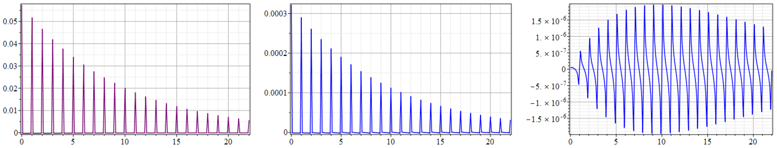
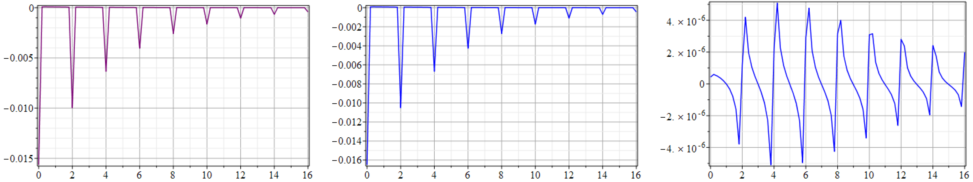
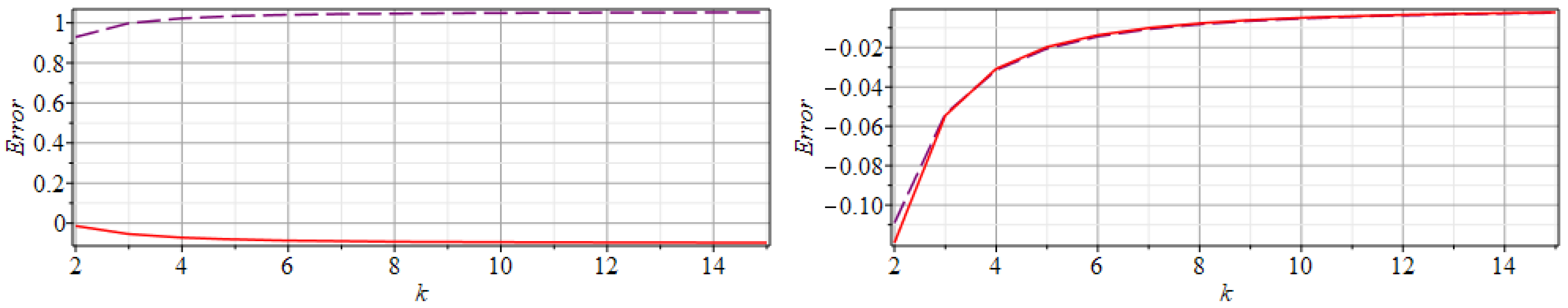
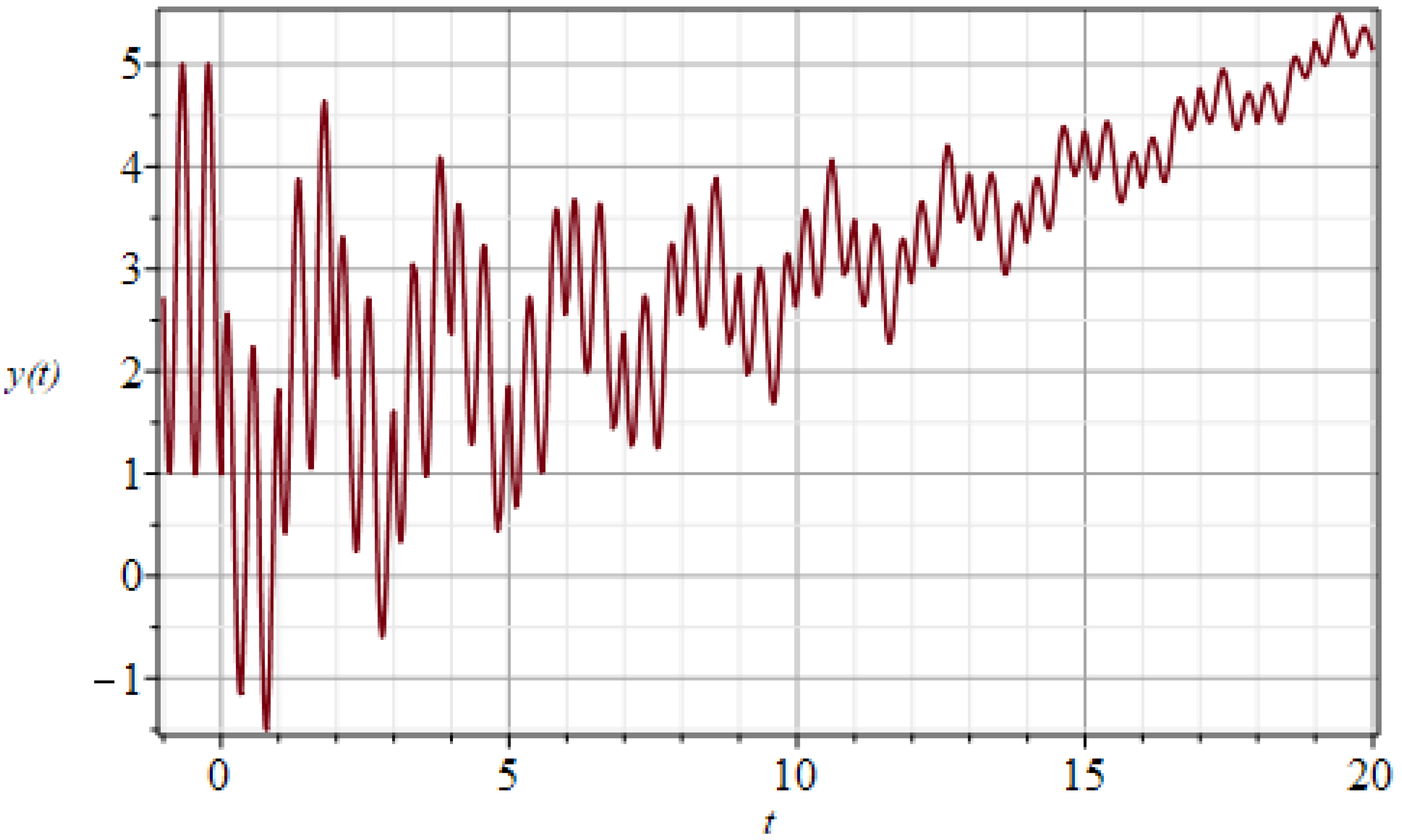
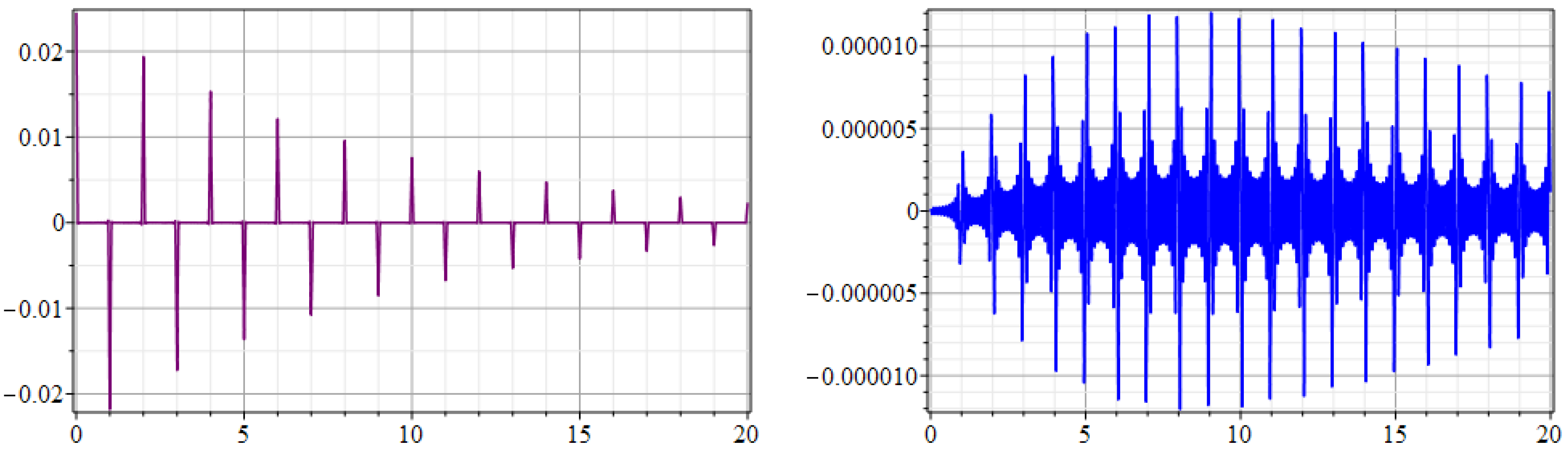
5. Illustrative Results of the New Higher-Order Convergence Laplace–Fourier Method

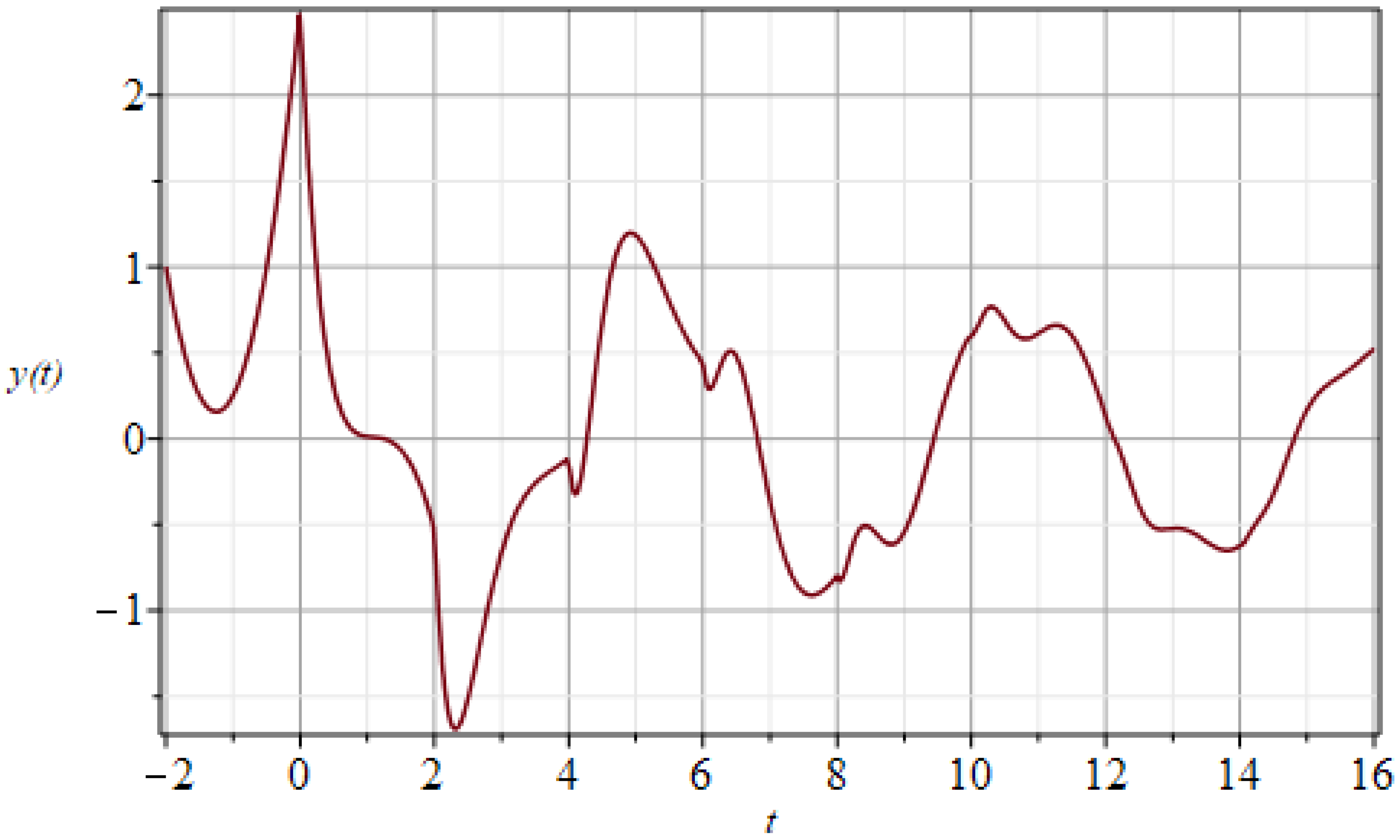
In this section, we will present a comparison between the pure Laplace and the new Laplace–Fourier methods by solving several NDDEs. We shall show that the developed method improves the accuracy of the Laplace solution without increasing the number of terms in the truncated series. In most of the examples, we will use the approximate formula for the location of the poles as our initial guess for determining the actual poles. In all of our examples, we include a graph of the analytic solution obtained via the MoS. In order to have fair comparisons between the methods, we use the same number of terms in each of the truncated series related to the methods. In addition, we include the error graphs for the solutions generated by the pure Laplace solution and the new Laplace–Fourier methods. The errors are obtained by computing the difference between the approximated solutions and the analytical solution over some finite time interval. We used Maple to perform all the required computations for the Laplace transform method, new Laplace–Fourier method, and the MoS. We compute the coefficients in the asymptotic expansions using Maple’s series command.

5.1. Example 1

Let us consider the following linear NDDE:

$$y^{\prime }\left(t\right)=-2.1y\left(t\right)+0.9y^{\prime }(t-1)+2.12y(t-1),H\left(t\right)=2-48t(1+t),t\in [-1,0].$$

(45)

We computed the solutions of NDDE (45) by the MoS (piecewise exact analytical solution), pure Laplace, original Laplace–Fourier, and the new Laplace–Fourier methods using the symbolic software Maple. For NDDE (45), there are two real poles: one negative ($r_0$) and one positive ($r_1$). Figure 1 shows the (oscillatory) solution obtained via the MoS. The solution may appear to approach a steady state, but it does not. It approaches $c_1{e}^{r_{1}t}$, where $r_1\approx 0.009$ and $c_1\approx 9.64$. Therefore, the solution of NDDE (45) increases exponentially, and there is no steady state. In Figure 2, the graphs of the absolute errors related to the different methods are presented. It is clear that the solution given by the new Laplace–Fourier method is the most accurate. While, as expected, the solution produced by the standard pure Laplace method is the least accurate. The accuracy can be further enhanced by increasing the number of terms in the series and/or by including more (higher degree) polynomials. The errors for all solutions decrease as the time increases, despite the fact that the solution itself is increasing. This is an important feature of all the implemented methods. For the absolute error plots, the peaks which occur at $t=k\tau$ are due to the nature of the non-harmonic series form of all the solutions generated by these methods [41,57]. It is important to remark that for all these methods once the solution is obtained, we can compute the solution for any time, even for a very large value of t, with a single calculation. In this example, polynomials of degree eight were used. We note, however, that for this particular example, the number of polynomials has a minimal effect in reducing the errors once we go beyond $p_3\left(x\right)$.

For the NNDE (45), we have that $ab+c=0.23$. On the left-hand side of Figure 3, we have plotted the relative errors of the real and imaginary parts computed using the correct residues $c_k$ versus the approximate values $c_k^a$, which were obtained from using the original Laplace–Fourier method. In particular, we show the graphs of $\mathfrak{Re}(c_k-c_k^a)/\mathfrak{Re}\left(c_k\right)$ and $\mathfrak{Im}(c_k-c_k^a)/\mathfrak{Im}\left(c_k\right)$ for $k=2\dots 12$. On the right-hand side of Figure 3, we have plotted the analogous errors, which were obtained from using the new Laplace–Fourier approximate values $c_k^a$ given by Equation (27).

5.2. Example 2

Let us consider the following linear NDDE:

$$y^{\prime }\left(t\right)=-2.1y\left(t\right)+{\displaystyle \frac{7}{11}}{y}^{\prime }(t-2)-2y(t-2),H\left(t\right)=1+{\displaystyle \frac{3}{2}}(t+2)(0.5+t),t\in [-2,0].$$

(46)

We computed the solutions of NDDE (46) by the MoS (piecewise exact analytical solution), pure Laplace, original Laplace–Fourier, and the new Laplace–Fourier methods. For NDDE (46), there are no real poles. In Figure 4, we show the solution computed by the MoS. In Figure 5, the graphs of the absolute errors related to the different methods are presented. Again, it is clear that the solution given by the new Laplace–Fourier method is the most accurate. In this example however, the solution produced by the original Laplace–Fourier method is slightly less accurate. This is due to the fact that there is a significant error in the asymptotic expansion for the residues $c_k$. However, the solution generated by the new Laplace–Fourier method is highly accurate due to the improvement in the computation of the residues, which is one of the main results of this paper. As usual, more accuracy can be obtained if the number of terms in the solutions are increased and/or more polynomials are included. The errors for all solutions decrease as time increases [41,57]. In this example, polynomials of degree eight were used.

For NNDE (46), we have that $ab+c=-367/110$. On the left-hand side of Figure 6, we have plotted the relative errors of the real and imaginary parts computed using the correct residues $c_k$ versus the approximate values $c_k^a$ which were obtained from using the original Laplace–Fourier method. In particular, we show the graphs of $\mathfrak{Re}(c_k-c_k^a)/\mathfrak{Re}\left(c_k\right)$ and $\mathfrak{Im}(c_k-c_k^a)/\mathfrak{Im}\left(c_k\right)$ for $k=2\dots 12$. On the right-hand side of Figure 6, we have plotted the analogous errors which were obtained from using the new Laplace–Fourier approximate values $c_k^a$ given by Equation (27).

5.3. Example 3

The last NDDE that we consider includes a periodic history function and also considers a coefficient $b<0$. Recall that for this particular case, the formulas for the approximate poles, frequencies, polynomials, etc., are different [57]. The NDDE is the following:

$$y^{\prime }\left(t\right)={\displaystyle \frac{14}{33}}y\left(t\right)-{\displaystyle \frac{8}{9}}{y}^{\prime }(t-1)-{\displaystyle \frac{1}{3}}y(t-1),H\left(t\right)=3-2cos14t,t\in [-1,0].$$

(47)

We computed the analytical solution of NDDE (47) in order to compare it with the solutions provided by the pure Laplace and the new Laplace–Fourier methods. For NDDE (47), there is one real pole (positive). Figure 7 shows the analytical solution given by the MoS. In Figure 8, the graphs of the absolute errors related to the pure Laplace and the new Laplace–Fourier methods are presented. It can be seen that the solution given by the new Laplace–Fourier method is significantly more accurate. This result is expected due to the fact that the new Laplace–Fourier method incorporates the improved asymptotic expansion for the residues.

In this example, we also show an important feature of the new Laplace–Fourier method. In Figure 9, we have plotted the error graphs for the pure Laplace and the new Laplace–Fourier solutions, but in this case, we increased the number of terms for the approximated solution (19) to $N=250$. Notice that the improvement in the new Laplace–Fourier method is considerably larger than the one of the pure Laplace method. We also note that Figure 8 and Figure 9 provide corroboration that the convergence rate for the new improved Laplace–Fourier method is $O\left(N^{-3}\right)$. We know the pure Laplace convergence rate is $O\left(N^{-1}\right)$. And we increased the number of terms in the series by a factor of 5. If we measure the corresponding error reduction based on the y-axis scales, we have an error reduction factor for the pure Laplace at $\approx 0.02/0.004=5$. However, the analogous error reduction factor for the improved Fourier–Laplace came out to $\approx 0.000012/(9.6\times {10}^{-8})=125$. In

Table 1. Maximum errors of the pure Laplace and the Laplace–Fourier methods for different values of terms N. Also, the convergence rates for each of the methods are shown.

Error
N	Pure Laplace	Convergence	New Laplace–Fourier	Convergence
50	$\approx 0.02$	$O\left(N^{-1}\right)$	$\approx 1.2\times {10}^{-5}$	$O\left(N^{-3}\right)$
250	$\approx 0.004$	$O\left(N^{-1}\right)$	$\approx 9.6\times {10}^{-8}$	$O\left(N^{-3}\right)$
500	$\approx 0.002$	$O\left(N^{-1}\right)$	$\approx 1.2\times {10}^{-8}$	$O\left(N^{-3}\right)$

, we present the maximum errors of the pure Laplace and the Laplace–Fourier methods. We have also, however, included the error for $N=500$. It is clear that the Laplace–Fourier method has a much better convergence rate than the pure Laplace method. In this example, polynomials of degree seven were used. And, although not included here, similar results were also observed for the NDDEs (45) and (46). Notice that once the Laplace–Fourier solution is obtained, it can be evaluated at any value of t with a very low computational time, which is a main advantage in comparison with numerical methods.

6. Conclusions

In this article, we have developed a new higher-order convergence Laplace–Fourier method to obtain solutions of linear NDDEs. This new method still combines the Laplace transform and Fourier series theory to obtain the solutions. However, by deriving and implementing an improved formula for the asymptotic expansion, for the residues, we were able to obtain more accurate solutions. The newly developed higher-order convergence Laplace–Fourier method generates more accurate solutions than the ones generated by the pure Laplace method and the original Laplace–Fourier method. We have shown that the convergence rate of the new Laplace–Fourier solution has a remarkable order of convergence at $O\left(N^{-3}\right)$. Examples and different comparisons with other methods have illustrated the accuracy of the new developed method. We have implemented the new method using the well-known Maple computer algebra software, but it can also be implemented with other available symbolic software such as Mathematica or Maxima. An improved approximate for the location of the complex poles that depends on all the parameters of the NDDEs was also derived. However, despite this more accurate approximation of the location of the poles, this cannot be used for the Laplace–Fourier methods. Nevertheless, we have shown that using the formula for the approximated location of poles that only depends on b and the time delay $\tau$ still produces a convergence rate of $O\left(N^{-3}\right)$. For particular NDDEs where b is very small in comparison with a and c, we can then use more terms in the Laplace–Fourier solution, and the accuracy of the analytical Laplace–Fourier solution can be increased.

We have shown that the solutions generated by the new higher-order convergence Laplace–Fourier method were very close to the analytical ones, with impressively small errors. Moreover, the errors effectively become negligible as t increases. It is important to remark that all of the advantageous features from the original Laplace–Fourier method are retained. For instance, the solution still accounts for the terms in the tail of the series, but now in a much more effective manner. And the accuracy of the solution can be increased by increasing the number of terms in the series and/or increasing the degree of the polynomials in the piecewise function. Furthermore, the Laplace–Fourier method generates a solution over the entire time domain, thus enabling one to compute the solution at any time with a single calculation. This is a main advantage in comparison with methods that generate numerical solutions. There are a variety of methods to obtain numerical solutions, and some mathematical specialized software have implemented them [58,59]. It has been shown in previous works that analytical solutions developed using the Laplace and the regular Laplace–Fourier methods are oftentimes more accurate than the numerical ones [41,57,60]. Since the higher-order convergence Laplace–Fourier method produces even more accurate solutions, we have obtained a large improvement regarding accuracy, which is a main contribution of this paper.

Finally, the solution given by the new higher-order convergence Laplace–Fourier method improves at a much larger rate than the one of the pure Laplace method. This is an excellent additional advantage of the new Laplace–Fourier method. The validity of the technique is corroborated by means of various illustrative examples. In summary, the new Laplace–Fourier method is a highly efficient method for solving linear NDDEs.

References

1. Erneux, T. Applied Delay Differential Equations; Springer Science & Business Media: Berlin/Heidelberg, Germany, 2009; Volume 3. [Google Scholar]
2. Halanay, A.; Safta, C.A. A critical case for stability of equilibria of delay differential equations and the study of a model for an electrohydraulic servomechanism. Syst. Control Lett. 2020, 142, 104722. [Google Scholar] [CrossRef]
3. Nelson, P.W.; Murray, J.D.; Perelson, A.S. A model of HIV-1 pathogenesis that includes an intracellular delay. Math. Biosci. 2000, 163, 201–215. [Google Scholar] [PubMed]
4. Goubault, E.; Putot, S.; Sahlmann, L. Inner and outer approximating flowpipes for delay differential equations. In Proceedings of the International Conference on Computer Aided Verification, Oxford, UK, 14–17 July 2018; pp. 523–541. [Google Scholar]
5. Rihan, F.A. Delay Differential Equations and Applications to Biology; Springer: Berlin/Heidelberg, Germany, 2021. [Google Scholar]
6. Shampine, L.; Gahinet, P. Delay-differential-algebraic equations in control theory. Appl. Numer. Math. 2006, 56, 574–588. [Google Scholar] [CrossRef]
7. Smith, H.L. An Introduction to Delay Differential Equations with Applications to the Life Sciences; Springer: New York, NY, USA, 2011; Volume 57. [Google Scholar]
8. Hethcote, H. Mathematics of infectious diseases. SIAM Rev. 2005, 42, 599–653. [Google Scholar]
9. Xu, R. Global dynamics of an {SEIS} epidemiological model with time delay describing a latent period. Math. Comput. Simul. 2012, 85, 90–102. [Google Scholar]
10. Hethcote, H.; Driessche, P. An SIS epidemic model with variable population size and a delay. J. Math. Biol. 1995, 34, 177–194. [Google Scholar] [CrossRef]
11. Yan, P.; Liu, S. SEIR epidemic model with delay. ANZIAM J. 2006, 48, 119–134. [Google Scholar]
12. Guo, B.Z.; Cai, L.M. A note for the global stability of a delay differential equation of hepatitis B virus infection. Math. Biosci. Eng. 2011, 8, 689–694. [Google Scholar]
13. Samanta, G. Dynamic behaviour for a nonautonomous heroin epidemic model with time delay. J. Appl. Math. Comput. 2011, 35, 161–178. [Google Scholar] [CrossRef]
14. Li, J.; Sun, G.Q.; Jin, Z. Pattern formation of an epidemic model with time delay. Phys. A Stat. Mech. Its Appl. 2014, 403, 100–109. [Google Scholar]
15. González-Parra, G.; Sultana, S.; Arenas, A.J. Mathematical modeling of toxoplasmosis considering a time delay in the infectivity of oocysts. Mathematics 2022, 10, 354. [Google Scholar] [CrossRef]
16. Aljahdaly, N.H.; El-Tantawy, S. On the multistage differential transformation method for analyzing damping Duffing oscillator and its applications to plasma physics. Mathematics 2021, 9, 432. [Google Scholar] [CrossRef]
17. Arino, J.; Van Den Driessche, P. Time delays in epidemic models. In Delay Differential Equations and Applications; Springer: Berlin/Heidelberg, Germany, 2006; pp. 539–578. [Google Scholar]
18. Bellen, A.; Guglielmi, N.; Ruehli, A.E. Methods for linear systems of circuit delay differential equations of neutral type. IEEE Trans. Circuits Syst. I Fundam. Theory Appl. 1999, 46, 212–215. [Google Scholar] [CrossRef]
19. Keane, A.; Krauskopf, B.; Postlethwaite, C.M. Climate models with delay differential equations. Chaos Interdiscip. J. Nonlinear Sci. 2017, 27, 114309. [Google Scholar] [CrossRef]
20. Ruehli, A.; Antonini, G.; Ekman, J. Neutral delay differential equations from the PEEC circuit solution of Maxwell’s equation. IFAC Proc. Vol. 2006, 39, 217–222. [Google Scholar] [CrossRef]
21. Inoue, T.; Katsui, T.; Rheem, C.K.; Yoshida, Z.; Matsuo, M.Y. Preliminary Study on Stick-Slip in Drillstring With Analytical Model Expressed With Neutral Delay Differential Equation. In Proceedings of the International Conference on Offshore Mechanics and Arctic Engineering, San Francisco, CA, USA, 8–13 June 2014; Volume 45462, p. V06AT04A026. [Google Scholar]
22. Boucekkine, R.; Pintus, P.A. History’s a curse: Leapfrogging, growth breaks and growth reversals under international borrowing without commitment. J. Econ. Growth 2012, 17, 27–47. [Google Scholar] [CrossRef]
23. Bachar, M. On periodic solutions of delay differential equations with impulses. Symmetry 2019, 11, 523. [Google Scholar] [CrossRef]
24. Biçer, E. On the periodic solutions of third-order neutral differential equation. Math. Methods Appl. Sci. 2021, 44, 2013–2020. [Google Scholar] [CrossRef]
25. Bicer, E. On the asymptotic behavior of solutions of neutral mixed type differential equations. Results Math. 2018, 73, 144. [Google Scholar] [CrossRef]
26. Breda, D.; Maset, S.; Vermiglio, R. Stability of Linear Delay Differential Equations: A Numerical Approach with MATLAB; Springer: Berlin/Heidelberg, Germany, 2014. [Google Scholar]
27. Faria, T.; Oliveira, J.J. Existence of positive periodic solutions for scalar delay differential equations with and without impulses. J. Dyn. Differ. Equ. 2019, 31, 1223–1245. [Google Scholar] [CrossRef]
28. He, J.H. Periodic solutions and bifurcations of delay-differential equations. Phys. Lett. A 2005, 347, 228–230. [Google Scholar]
29. Castro, M.Á.; García, M.A.; Martín, J.A.; Rodríguez, F. Exact and nonstandard finite difference schemes for coupled linear delay differential systems. Mathematics 2019, 7, 1038. [Google Scholar] [CrossRef]
30. García, M.; Castro, M.; Martín, J.A.; Rodríguez, F. Exact and nonstandard numerical schemes for linear delay differential models. Appl. Math. Comput. 2018, 338, 337–345. [Google Scholar]
31. Gumgum, S.; Savasaneril, N.B.; Kurkcu, O.; Sezer, M. Lucas polynomial solution for neutral differential equations with proportional delays. TWMS J. Appl. Eng. Math. 2020, 10, 259–269. [Google Scholar]
32. Jamilla, C.U.; Mendoza, R.G.; Mendoza, V.M.P. Explicit solution of a Lotka-Sharpe-McKendrick system involving neutral delay differential equations using the r-Lambert W function. Math. Biosci. Eng. 2020, 17, 5686–5708. [Google Scholar] [PubMed]
33. Jamilla, C.; Mendoza, R.; Mezo, I. Solutions of neutral delay differential equations using a generalized Lambert W function. Appl. Math. Comput. 2020, 382, 125334. [Google Scholar] [CrossRef]
34. Kumar, M. An Efficient Numerical Scheme for Solving a Fractional-Order System of Delay Differential Equations. Int. J. Appl. Comput. Math. 2022, 8, 262. [Google Scholar] [CrossRef]
35. Luo, X.; Habib, M.; Karim, S.; Wahash, H.A. Semianalytical approach for the approximate solution of delay differential equations. Complexity 2022, 2022. [Google Scholar]
36. Senu, N.; Ahmad, N.A.; Othman, M.; Ibrahim, Z.B. Numerical study for periodical delay differential equations using Runge–Kutta with trigonometric interpolation. Comput. Appl. Math. 2022, 41, 25. [Google Scholar]
37. Bauer, R.J.; Mo, G.; Krzyzanski, W. Solving delay differential equations in S-ADAPT by method of steps. Comput. Methods Programs Biomed. 2013, 111, 715–734. [Google Scholar] [CrossRef]
38. Kalmár-Nagy, T. Stability analysis of delay-differential equations by the method of steps and inverse Laplace transform. Differ. Equ. Dyn. Syst. 2009, 17, 185–200. [Google Scholar]
39. Kaslik, E.; Sivasundaram, S. Analytical and numerical methods for the stability analysis of linear fractional delay differential equations. J. Comput. Appl. Math. 2012, 236, 4027–4041. [Google Scholar]
40. Heffernan, J.M.; Corless, R.M. Solving some delay differential equations with computer algebra. Math. Sci. 2006, 31, 21–34. [Google Scholar]
41. Kerr, G.; González-Parra, G. Accuracy of the Laplace transform method for linear neutral delay differential equations. In Mathematics and Computers in Simulation; Elsevier: Amsterdam, The Netherlands, 2022. [Google Scholar]
42. Bazighifan, O.; Alotaibi, H.; Mousa, A.A.A. Neutral delay differential equations: Oscillation conditions for the solutions. Symmetry 2021, 13, 101. [Google Scholar] [CrossRef]
43. Fabiano, R.H.; Payne, C. Spline approximation for systems of linear neutral delay-differential equations. Appl. Math. Comput. 2018, 338, 789–808. [Google Scholar]
44. Fabiano, R.H. A semidiscrete approximation scheme for neutral delay-differential equations. Int. J. Numer. Anal. Model. 2013, 10. [Google Scholar]
45. Faheem, M.; Raza, A.; Khan, A. Collocation methods based on Gegenbauer and Bernoulli wavelets for solving neutral delay differential equations. Math. Comput. Simul. 2021, 180, 72–92. [Google Scholar]
46. Liu, M.; Dassios, I.; Milano, F. On the stability analysis of systems of neutral delay differential equations. Circuits Syst. Signal Process. 2019, 38, 1639–1653. [Google Scholar]
47. Qin, H.; Zhang, Q.; Wan, S. The continuous Galerkin finite element methods for linear neutral delay differential equations. Appl. Math. Comput. 2019, 346, 76–85. [Google Scholar]
48. Philos, C.G.; Purnaras, I. Periodic first order linear neutral delay differential equations. Appl. Math. Comput. 2001, 117, 203–222. [Google Scholar]
49. Raza, A.; Khan, A. Haar wavelet series solution for solving neutral delay differential equations. J. King Saud Univ.-Sci. 2019, 31, 1070–1076. [Google Scholar] [CrossRef]
50. Santra, S.S.; Nofal, T.A.; Alotaibi, H.; Bazighifan, O. Oscillation of Emden–Fowler-Type Neutral Delay Differential Equations. Axioms 2020, 9, 136. [Google Scholar] [CrossRef]
51. Gu, K.; Niculescu, S.I. Survey on recent results in the stability and control of time-delay systems. J. Dyn. Sys. Meas. Control 2003, 125, 158–165. [Google Scholar] [CrossRef]
52. Kim, B.; Kwon, J.; Choi, S.; Yang, J. Feedback stabilization of first order neutral delay systems using the Lambert W function. Appl. Sci. 2019, 9, 3539. [Google Scholar] [CrossRef]
53. Kuang, Y. Delay Differential Equations; University of California Press: Berkeley, CA, USA, 2012. [Google Scholar]
54. Xu, Q.; Stepan, G.; Wang, Z. Balancing a wheeled inverted pendulum with a single accelerometer in the presence of time delay. J. Vib. Control 2017, 23, 604–614. [Google Scholar] [CrossRef]
55. Enright, W.; Hayashi, H. Convergence analysis of the solution of retarded and neutral delay differential equations by continuous numerical methods. SIAM J. Numer. Anal. 1998, 35, 572–585. [Google Scholar] [CrossRef]
56. Xu, X.; Huang, Q.; Chen, H. Local superconvergence of continuous Galerkin solutions for delay differential equations of pantograph type. J. Comput. Math 2016, 34, 186–199. [Google Scholar]
57. Kerr, G.; González-Parra, G.; Sherman, M. A new method based on the Laplace transform and Fourier series for solving linear neutral delay differential equations. Appl. Math. Comput. 2022, 420, 126914. [Google Scholar] [CrossRef]
58. Shampine, L.F.; Thompson, S. Solving ddes in matlab. Appl. Numer. Math. 2001, 37, 441–458. [Google Scholar] [CrossRef]
59. Shampine, L.F.; Thompson, S. Numerical solution of delay differential equations. In Delay Differential Equations; Springer: Berlin/Heidelberg, Germany, 2009; pp. 1–27. [Google Scholar]
60. Sherman, M.; Kerr, G.; González-Parra, G. Comparison of Symbolic Computations for Solving Linear Delay Differential Equations Using the Laplace Transform Method. Math. Comput. Appl. 2022, 27, 81. [Google Scholar] [CrossRef]
61. Golmankhaneh, A.K.; Tejado, I.; Sevli, H.; Valdés, J.E.N. On initial value problems of fractal delay equations. Appl. Math. Comput. 2023, 449, 127980. [Google Scholar]
62. Kerr, G.; Lopez, N.; González-Parra, G. Analytical Solutions of Systems of Linear Delay Differential Equations by the Laplace Transform: Featuring Limit Cycles. Math. Comput. Appl. 2024, 29, 11. [Google Scholar] [CrossRef]
63. Hale, J.K.; Lunel, S.M.V. Introduction to Functional Differential Equations; Springer Science & Business Media: Berlin/Heidelberg, Germany, 2013; Volume 99. [Google Scholar]
64. Kuang, Y. Delay Differential Equations: With Applications in Population Dynamics; Academic Press: Cambridge, MA, USA, 1993. [Google Scholar]
65. Diekmann, O.; Van Gils, S.A.; Lunel, S.M.; Walther, H.O. Delay Equations: Functional-, Complex-, and Nonlinear Analysis; Springer Science & Business Media: Berlin/Heidelberg, Germany, 2012; Volume 110. [Google Scholar]
66. Sherman, M.; Kerr, G.; González-Parra, G. Analytical solutions of linear delay-differential equations with Dirac delta function inputs using the Laplace transform. Comput. Appl. Math. 2023, 42, 268. [Google Scholar] [CrossRef]
67. Brown, J.W.; Churchill, R.V. Fourier Series and Boundary Value Problems; McGraw-Hill Book Company: New York, NY, USA, 2009. [Google Scholar]
68. Oberhettinger, F. Fourier Expansions: A Collection of Formulas; Elsevier: Amsterdam, The Netherlands, 2014. [Google Scholar]
Figure 1. Analytical solution obtained by the MoS. The NDDE is y ( t ) = 2.1 y ( t ) + 0.9 y ( t 1 ) + 2.12 y ( t 1 ) , H ( t ) = 2 48 t ( 1 + t ) , t [ 1 , 0 ] .
Mca 30 00037 g001
Figure 2. Errors of the solutions obtained by pure Laplace (left), original Laplace–Fourier (center), and the new Laplace–Fourier (right) methods. The NDDE is y ( t ) = 2.1 y ( t ) + 0.9 y ( t 1 ) + 2.12 y ( t 1 ) , H ( t ) = 2 48 t ( 1 + t ) , t [ 1 , 0 ] .
Mca 30 00037 g002
Figure 3. Relative errors of the imaginary (solid lines) and real (dashed lines) parts using the correct residues c k versus the approximate values c k a for the original Laplace–Fourier (left) and for the new Laplace–Fourier method (right). The NDDE is y ( t ) = 2.1 y ( t ) + 0.9 y ( t 1 ) + 2.12 y ( t 1 ) , H ( t ) = 2 48 t ( 1 + t ) , t [ 1 , 0 ] .
Mca 30 00037 g003
Figure 4. Analytical solution obtained by the MoS. The NDDE is y ( t ) = 2.1 y ( t ) + 7 11 y ( t 2 ) 2 y ( t 2 ) , H ( t ) = 1 + 3 2 ( t + 2 ) ( 0.5 + t ) , t [ 2 , 0 ] .
Mca 30 00037 g004
Figure 5. Errors of the solutions obtained by pure Laplace (left), original Laplace–Fourier (center), and the new Laplace–Fourier (right) methods. The NDDE is y ( t ) = 2.1 y ( t ) + 7 11 y ( t 2 ) 2 y ( t 2 ) , H ( t ) = 1 + 3 2 ( t + 2 ) ( 0.5 + t ) , t [ 2 , 0 ] .
Mca 30 00037 g005
Figure 6. Relative errors of the imaginary (solid lines) and real (dashed lines) parts using the correct residues c k versus the approximate values c k a for the original Laplace–Fourier (left) and for the new Laplace–Fourier method (right). The NDDE is y ( t ) = 2.1 y ( t ) + 0.9 y ( t 1 ) + 2.12 y ( t 1 ) , H ( t ) = 2 48 t ( 1 + t ) , t [ 1 , 0 ] .
Mca 30 00037 g006
Figure 7. Analytical solution obtained by the MoS. The NDDE is y ( t ) = 14 33 y ( t ) 8 9 y ( t 1 ) 1 3 y ( t 1 ) , H ( t ) = 3 2 cos 14 t , t [ 1 , 0 ] .
Mca 30 00037 g007
Figure 8. Errors of the solutions obtained by pure Laplace (left) and the new Laplace–Fourier (right) methods. The NDDE is y ( t ) = 14 33 y ( t ) 8 9 y ( t 1 ) 1 3 y ( t 1 ) , H ( t ) = 3 2 cos 14 t , t [ 1 , 0 ] . The number of terms used to compute the approximated solution (19) is N = 50 .
Mca 30 00037 g008
Figure 9. Relative errors of the imaginary (left) and real (right) parts using the correct residues c k versus the approximate values c k a for the original Laplace–Fourier (solid lines) and for the new Laplace–Fourier method (dashed lines). The NDDE is y ( t ) = 14 33 y ( t ) 8 9 y ( t 1 ) 1 3 y ( t 1 ) , H ( t ) = 3 2 cos 14 t , t [ 1 , 0 ] . The number of terms used to compute the approximated solution (19) is N = 250 .
Mca 30 00037 g009