Abstract
This paper presents a trajectory-tracking controller of an inverted pendulum system on a self-balancing differential drive platform. First, the system modeling is described by considering approximations of the swing angles. Subsequently, a discrete convex representation of the system via the nonlinear sector technique is obtained, which considers the nonlinearities associated with the nonholonomic constraint. The design of a discrete parallel distributed compensation controller is achieved through an alternative method due to the presence of uncontrollable points that avoid finding a solution for the entire polytope. Finally, simulations and experimental results using a prototype illustrate the effectiveness of the proposal.
1. Introduction
The control of critical systems is an important area of study in robotics, as these systems operate around unstable equilibrium points; once they reach a critical zone, it is impossible to re-stabilize them due to physical limitations in their actuators; a classic example is the inverted pendulum on a self-balancing platform. The main challenge lies in maintaining two coupled joints within the allowable limits of the equilibrium point despite the inevitable presence of measurement noise, disturbances, and model inaccuracies [1,2]. One way to prevent the system from going beyond its bounds is using constrained predictive control strategies [3,4]. However, these strategies come with high computational costs, making them prohibitive for most of the low-cost embedded hardware.
As the balancing platform is essentially a mobile robot with differential traction, movement restrictions arise due to its nonholonomic nature, adding complexity and turning it into a multi-objective problem. Balance must be maintained while following a specific trajectory on the plane, which poses significant challenges in planning and control execution [5]. The literature covers various subjects: hardware, sensing configurations, and control methods for two-wheeled and self-balancing robots [6,7,8]. For instance, the authors in [1] introduced a low-cost prototype with nested control to regulate the longitudinal displacement and speed via the pitch angle. In [9,10], advanced control algorithms are proposed using adaptive sliding mode and direct fuzzy control for improved velocity tracking and stability. The works [11,12] presented a nonlinear control approach, avoiding linearization around the equilibrium points; a machine-learning-based adaptive fuzzy logic-proportional integral controller for variable payloads in a two-wheeled underactuated-mobile inverted pendulum was developed by [13]. Recently, refs. [14,15] proposed a self-balancing robot with PID control using sensors and complementary filters for practical angular velocity estimation and motor stability; the controller was implemented with Arduino. However, to the best of the authors’ knowledge, few works have been dedicated to the study of two-wheeled and self-balancing platforms with a coupled inverted pendulum.
This paper presents the model and control of the inverted pendulum coupled with a two-wheeled and self-balancing differential robot. The model is developed under specific considerations, thus, allowing for simplifications without losing accuracy within the operating region. A discrete parallel distributed compensation (PDC) controller is designed for control and trajectory tracking based on an exact convex model [16]. Experimental results are presented to illustrate the performance of the proposed method.
The rest of the paper is organized as follows: Section 2 outlines the fundamental concepts and the problem to be solved. Section 3 presents the main results related to obtaining the mathematical model and controller design. Section 4 illustrates the performance of the proposed control scheme by means of simulations, while Section 5 validates the control strategy by means of an experimental test. Finally, Section 6 closes the paper with some final remarks and conclusions.
Preliminaries: Throughout the paper, the following notation will be employed: In the case of a matrix , and stand for the transpose and the inverse, respectively. Given the complex variable , represents its complex conjugate. Additionally, the symbol * indicates the transpose of the element in the symmetric position of the matrix.
2. Problem Statement
Consider the inverted pendulum system coupled to a two-wheeled and self-balancing mobile platform with differential traction, as displayed in Figure 1. This system can be modeled as a double inverted pendulum, which includes rotational motion and longitudinal movement. The differential traction mechanism allows the platform to follow a specific path. The control objective for the mobile platform is to track a desired reference signal while the pendulum is stabilized at the vertical position.
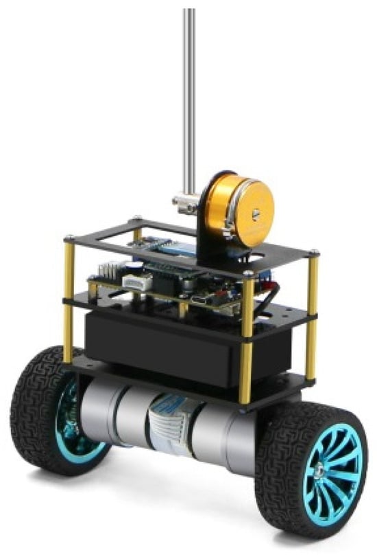
Figure 1.
Prototype of the inverted pendulum on a self-balancing differential robot.
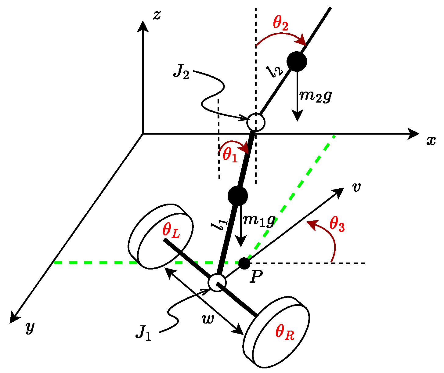
A free-body diagram of the system can be seen in Figure 2, where and represent the joints. In this case, joint couples the inverted pendulum with the cart and its pivotal, allowing the pendulum to swing while mounted on the mobile platform. The parameters and variables of this system are shown in Table 1.
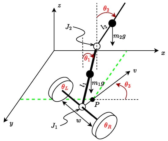
Figure 2.
Diagram of a self-balancing car with an inverted pendulum.

Table 1.
Relationship of parameters for the self-balancing cart model with an inverted pendulum.
Considering the Euler–Lagrange energy approach to model the longitudinal motion, where both wheels rotate together to stabilize the oscillating body. The energy equations for each wheel are defined by the following:
The potential energy for both is zero () as they remain on the horizontal plane. For the position of the cart (, ), the localization of the center of mass in the plane () of the joint (self-balancing) is represented by the following:
and the velocity of the center of mass :
As for the kinetic and potential energies at the joint , we have
which are equivalent to:
Similarly, for the joint (pendulum), its position and velocity in the plane (); are described by the following expressions:
Their kinetic and potential energies are obtained as follows:
by replacing and , we have:
Nonholonomic Model
The above equations do not consider the kinematic part of the nonholonomic inherent in the differential traction vehicle setup. Following [5], the model of the differential robot considering the displaced point is as follows:
where and are the wheel velocities. By considering these velocities, the angle can be computed in real-time using the following odometry equation:
Note that it is not possible to simultaneously control x, y, and due to the nonholonomic constraints; therefore, is treated as an exogenous parameter and the dynamic equation associated with is removed from (4). Now, let us consider the accelerations at each wheel and , an augmented system can be formulated with and ; it yields the following augmented nonlinear system:
Equations (1)–(3) describe the kinetic and potential energy of the tires and the joint together with the kinematic model (5); all of them will be used to solve the Euler–Lagrange equations describing the robot behavior. Here, the challenge is to design a tracking controller that maintains the vertical position of the joint while the differential cart follows a trajectory. The next section proposes a method for the design of a discrete-time PDC controller for trajectory tracking while guaranteeing stability.
3. Main Results
The proposed methodology assumes that the only energy contributing to the joint motion comes from the translation of the cart, with zero rotational energy at ; rotation about will only be considered in the kinematic part of the cart. Following the Euler–Lagrange modeling procedure, the kinetic energy can be expressed as and the potential energy as (from Equations (1), (2), and (3), respectively). The Lagrangian is then denoted as , where is the generalized coordinate.
Traditionally, the functional derivative is applied using a vector q together with the non-conservative forces acting on each joint; in this case, the torques applied to each wheel are considered [17]. However, a model with torques as the inputs could be more practical. This work assumes that each motor has an internal velocity controller, which is very common, as discussed in [18].
The vector of generalized coordinates is defined by and solving the Euler–Lagrange equation:
the solution for the generalized coordinates is obtained as follows:
Considering that angles and variate within a small range , the following approximations can be used:
hence, (6) and (7) yield:
where and represent the accelerations of each wheel that are considered as the control inputs. From (9) and (10), a system of first-order ordinary differential equations is obtained:
with:
Finally, by combining (5) and (11), a nonlinear model of the inverted pendulum on a self-balancing robot yields:
with:
Model (12) contains information about the kinematic aspect associated with the nonholonomic constraints and the dynamic longitudinal model related to self-balancing coupled with the inverted pendulum. Despite the small angle approximations, the model contains some nonlinearities related to the angle that will be handled in the next section by considering exact convex modeling.
Convex Controller Design
The nonlinear model (12) can be represented as a discrete convex Takagi–Sugeno (TS) model to simplify the controller design. This transformation is achieved using the nonlinear sector technique, as detailed in [16]. A convex representation is obtained by expressing the nonlinearities of the system as bounded functions. This rewriting of the nonlinear model allows us to design the controller by obtaining a numerical solution using Linear Matrix Inequalities (LMIs).
The resulting discrete convex model is given by the following:
where , , and are the state, input, and output vectors, respectively. The exogenous premise vector is , it is assumed to be bounded in a compact set , and the number of vertices is . Matrices , , and are the discrete equivalent matrix vertices computed utilizing the sector nonlinearity approach [16]. The membership functions , hold the convex sum property in : . Hence, as the entries of the premise vector have natural limits, we have ; then, the membership functions
are obtained with , , and .
For the control and stabilization of the system (13), the following PDC-type control law is employed
where , is the feedback gain to be designed.
As is customary in the convex community, the design of the feedback gains is carried out by quadratic Lyapunov functions ending in LMI conditions. However, the polytopic representation assumes independence among all terms of the vector . Because of coupling among these terms, regions within the compact set do not accurately belong to the model, leading to conservatism in the polytopic representation, as discussed in [19]. Specifically, the point within results in two critically uncontrollable poles, limiting an asymptotically stable solution for the entire .
Therefore, the values of for each vertex are computed by considering a Linear Quadratic Regulator (LQR). This approach allows for a straightforward adjustment of the cost matrices to attain the desired solution. The discrete-time LQR gains are calculated using the matrices Q and R to solve the optimization problem [20]:
As a stability test, an LMI region with a radius infinitesimally greater than unity to encompass the uncontrollable poles is considered through the following [21]:
where , , . These LMIs verify that all closed-loop system poles are within the circular region of radius . A non-negative slack variable is introduced to handle numerical issues arising from critically stable uncontrollable poles.
Remark 1.
Due to the presence of uncontrollable points within the polytope defined by the nonlinear terms and , it is not possible to find a direct solution for LMIs (14). This is a computational problem that arises from the specific structure of the model and avoids those standard LMI solvers finding a feasible solution. However, the system is controllable, and a solution must exist, even if the solver can not solve the LMI directly. The proposed approach computes the controller gains at the vertex of the polytope by considering an LQR. Then, with the computed gains, the LMI (14) is solved to prove the asymptotic stability. We acknowledge that obtaining a direct LMI solution would be ideal. Nonetheless, the proposed method provides an effective alternative for stabilizing the inverted pendulum system from a practical point of view.
4. Simulation Results
For the simulations and experimental tests, the parameters in Table 2 have been used; most of these parameters have been provided by the manufacturer, while others have been computed and estimated in the laboratory. Due to the characteristics of the prototype, a sampling time of is considered.
Table 2.
Parameters of the prototype.
To compute the LQR at each vertex, the following cost matrices have been used:
The weight matrices were adjusted empirically to balance the system performance and actuator power consumption. It should be noted that the proposed method primarily validates the stability of the convex gain configurations without ensuring optimal performance due to the presence of non-controllable points within the convex polytope. Some aspects, such as robustness, noise handling, and optimization of the weight matrices, are beyond the scope of this study. However, the stability of the system is verified by testing the LMI (14) with the computed gains, which guarantees asymptotic convergence of the desired tracking controller. The computed gains are:
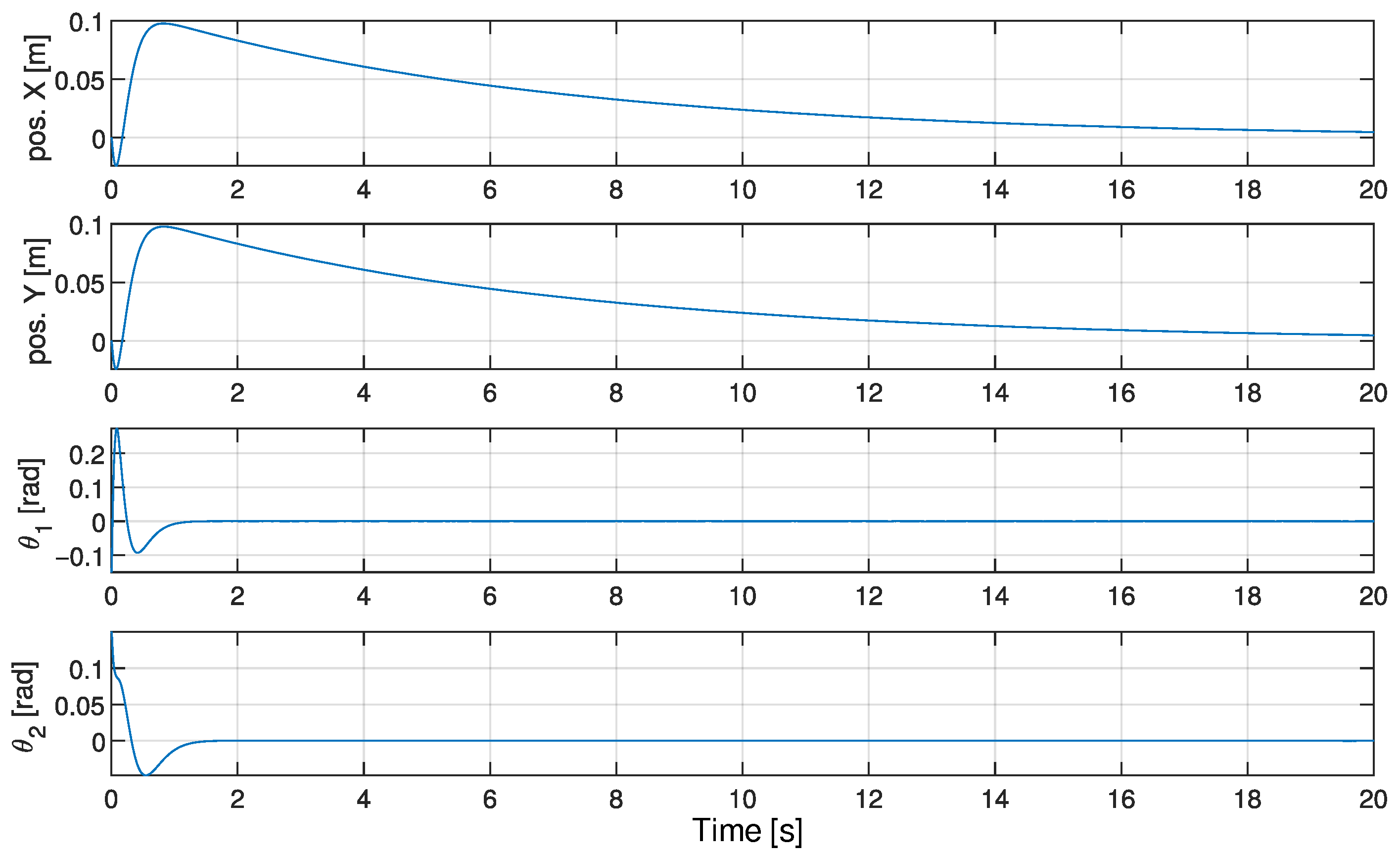
Simulation results illustrate the stabilization of the pendulum from an unstable initial position, and its return to the origin are presented in Figure 3. These simulations operate within the -degree range, consistent with the small-angle approximation. A Gaussian noise signal was also introduced into the control inputs to simulate possible disturbances. As can be seen in the figure, the controllers perform well, keeping the vertical position of the pendulum while maintaining the system at the origin.
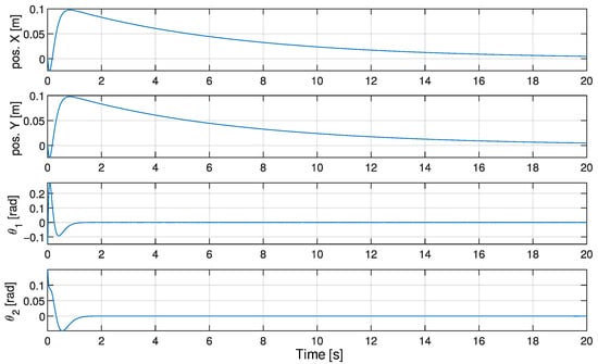
Figure 3.
Transient response for initial conditions at , , different from zero.
5. Experimental Results
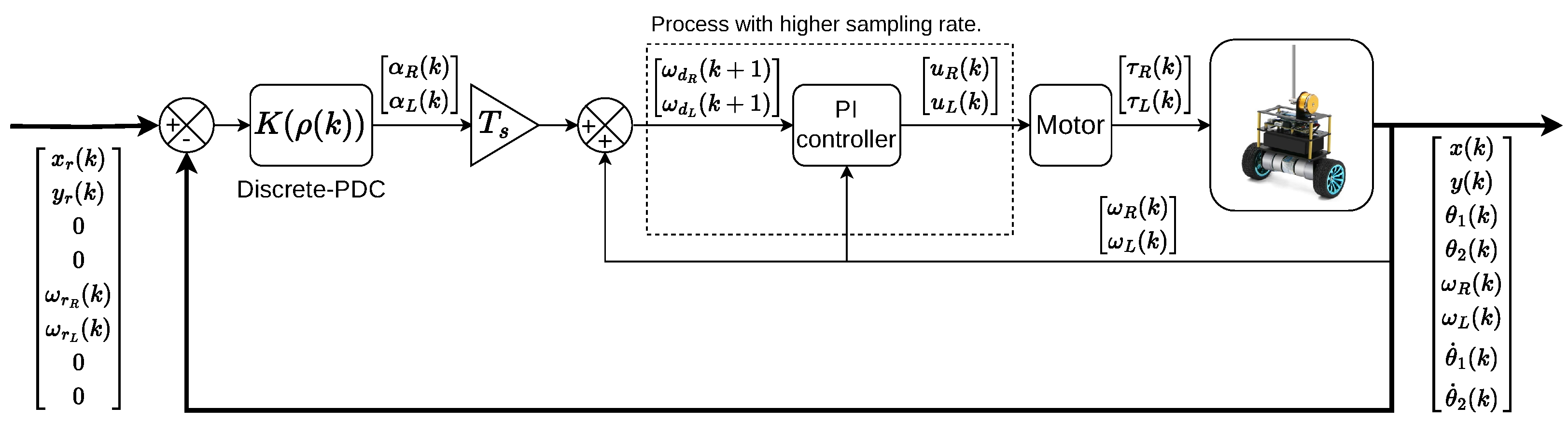
For practical implementation, the speed in each actuator is assumed to be controlled; in our case, the manufacturer provides a tuned PI controller to control the speed in each motor. Figure 4 shows a closed-loop system diagram of the proposal. As the output of the PDC controller is in terms of acceleration (rad/s2) at sampling instant , it is necessary to obtain the reference of velocity for the PI controller. To this end, a dynamic integrator is added. First, the PDC acceleration command is multiplied by the sampling time to obtain the required velocity increment at time in rad/s. This increment is added to the current velocity to obtain the reference velocity at . The PI controller is correctly tuned and uses a considerably smaller sampling period, inserting virtually negligible dynamics into the overall system.
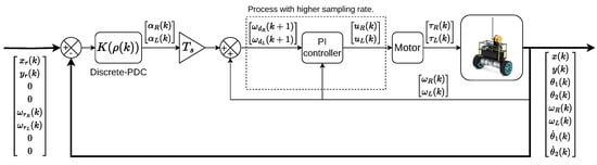
Figure 4.
Overall system diagram. Symbols and u represent the torque and voltage applied to each DC motor.
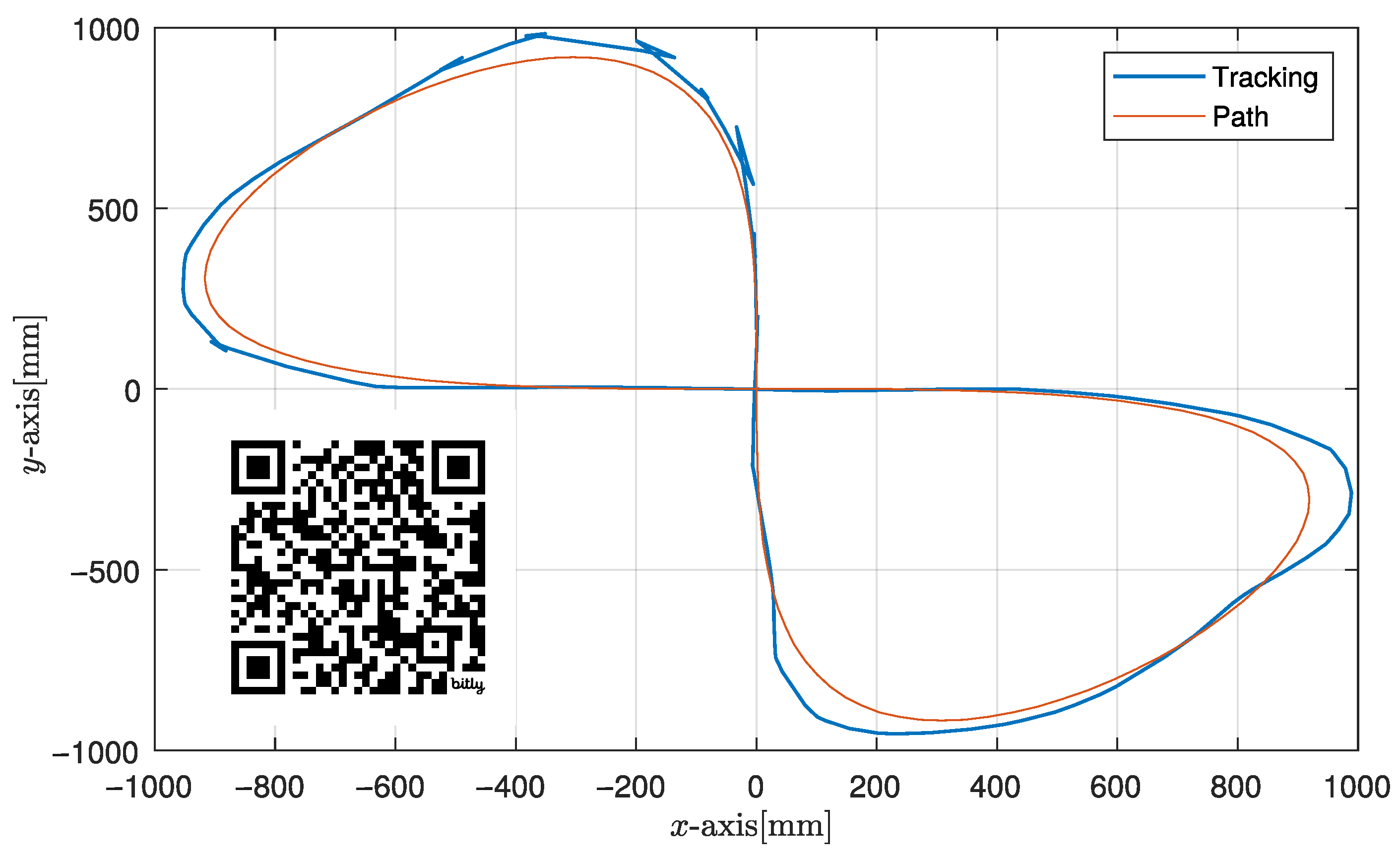
The algorithm has been programmed in the embedded system provided by the manufacturer, which consists of an STM32F103—Arm Cortex-M3 microcontroller. The data have been acquired through Bluetooth serial communication, with a sampling period of 500 ms. A lemniscate trajectory was considered as a reference. Details of how to implement this reference are given in Appendix A.
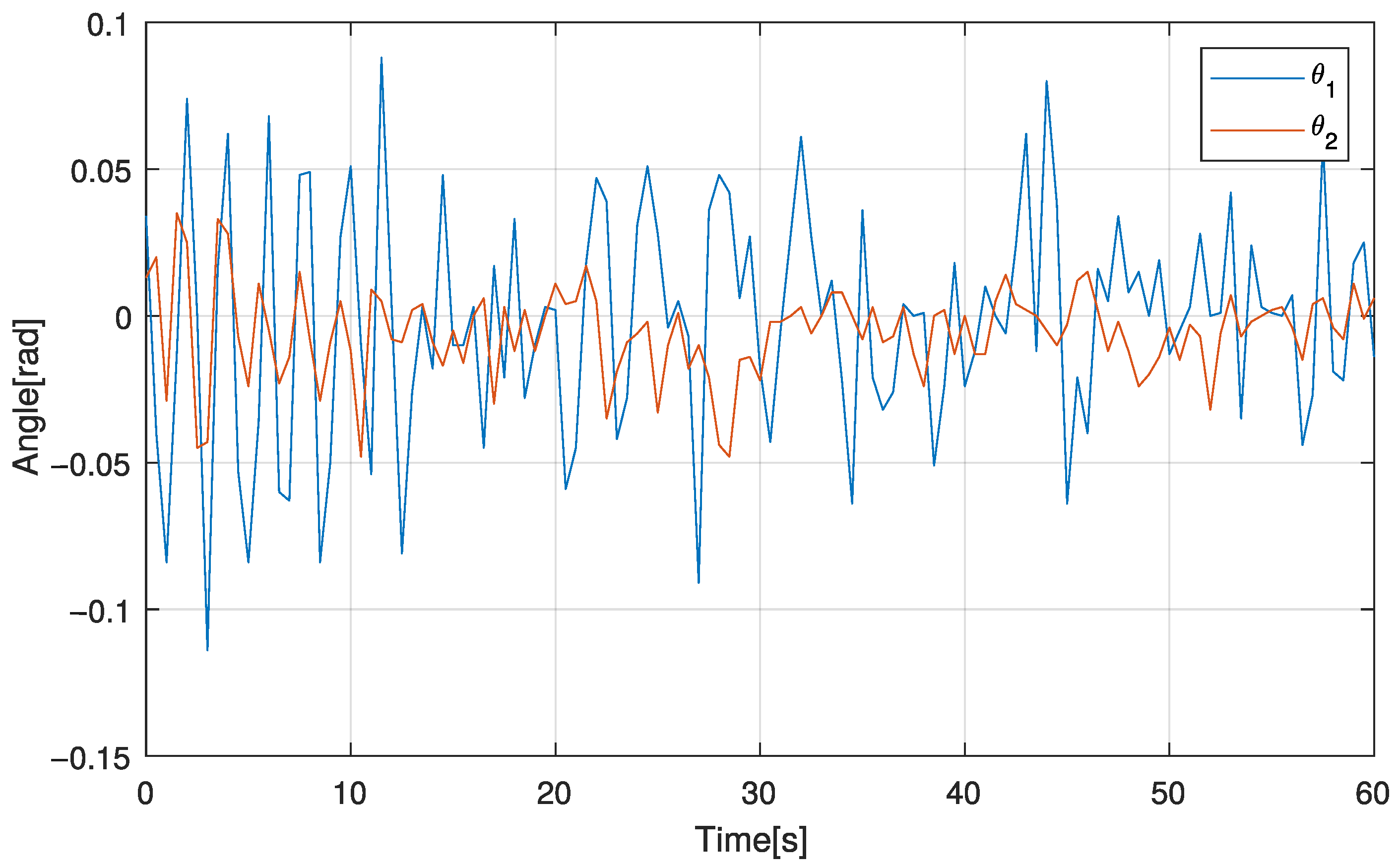
Figure 5 displays the trajectory tracking response, where a slight deviation can be seen in the curves due to the variations in the linear and angular velocities of the path. These deviations show the sensitivity of the system to path accelerations. Figure 6 illustrates the behavior of angles and during the 60 s of testing. In this case, noise is particularly noticeable at , mainly due to the IMU’s low quality and the potentiometer used to measure . However, despite the noise, the maximum deflection peaks remain within the designed values for the small angle approximations.
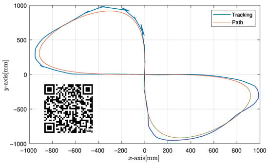
Figure 5.
Experimental trajectory tracking.
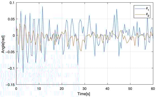
Figure 6.
Transient behavior of the angles and .
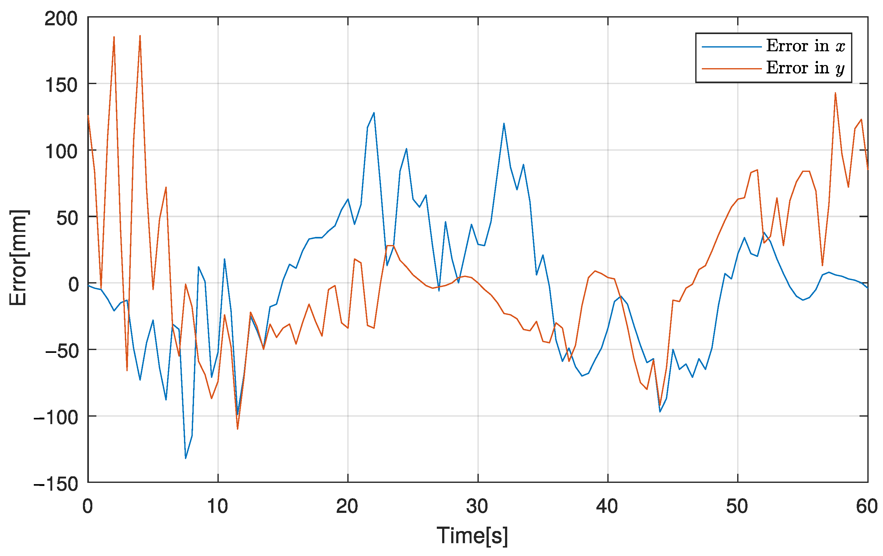
Figure 7 shows the errors concerning x and y obtained in the tracking test. Instantaneous deviations are observed due to the continuous effort to stabilize the cart, the pendulum, and the sensor noise. The different plots illustrate that the control system design implies a compromise between tracking error reduction and system stability. A video of the experimental test can be consulted at the link: https://bit.ly/gturixpendubot (accessed on 16 September 2024).
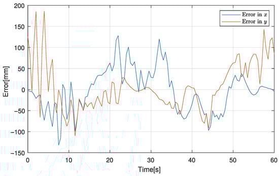
Figure 7.
Transient behavior of the trajectory tracking error in the x and y axes.
6. Conclusions
A convex approach has been considered for modeling and controlling an inverted pendulum coupled with a self-balancing differential drive cart. The adopted control approach is practical for satisfactorily managing the nonholonomic constraints in the differential drive kinematic model of the cart, as stability and trajectory tracking have been achieved. Regardless of the noise and disturbances, the system presents an adequate response, which is demonstrated to be robust and practical. The main drawback encountered was the impossibility of finding a feasible solution for the LMIs due to uncontrollable points that appear due to the nonholonomic system. This led to exploring an alternative solution using LQR, followed by stability verification. Future work will focus on improving the controller’s robustness and performance, optimizing its ability to handle system disturbances and uncertainties, and considering more advanced LMI techniques.
Author Contributions
Conceptualization, Y.G.-C. and F.-R.L.-E.; methodology, Y.G.-C., F.-R.L.-E. and V.E.-M.; software, F.-R.L.-E.; validation, Y.G.-C. and F.-R.L.-E.; formal analysis, F.-R.L.-E., Y.G.-C. and V.E.-M.; investigation, Y.G.-C.; resources, J.D.-Z.; data curation, Y.G.-C. and M.L.-P.; writing—original draft preparation, Y.G.-C.; writing—review and editing, Y.G.-C., F.-R.L.-E. and V.E.-M.; supervision, project administration and funding acquisition, J.D.-Z. and F.-R.L.-E. All authors have read and agreed to the published version of the manuscript.
Funding
This research was funded by Tecnológico Nacional de México (TecNM) and Consejo Nacional de Humanidades, Ciencias y Tecnologías (CONAHCYT) in Mexico.
Data Availability Statement
The raw data supporting the conclusions of this article will be made available by the the authors upon request.
Acknowledgments
This research was supported by Tecnológico Nacional de México through the Proyectos de Investigación Científica call and by the National Council of Humanities, Science, and Technologies (CONAHCYT) under the national scholarship program. The authors are grateful for the scientific support provided by the RICCA network (Red Internacional de Control y Cómputo Aplicados). We also extend our appreciation to the anonymous reviewers for their valuable feedback, which has significantly contributed to improving the quality of this paper.
Conflicts of Interest
The authors declare no conflicts of interest.
Appendix A
The experiment utilized a lemniscate trajectory, mathematically described by the following equations:
where and represent the maximum amplitude on the respective axis, is the angular frequency, and is the period to traverse one complete cycle of the trajectory.
The linear velocity at each instant of the path, , is given by:
where the velocity components and are:
The angle of the velocity vector is calculated as:
and the angular velocity is derived as:
The inverse kinematics for determining the reference velocity at each wheel are expressed as:
where w is the distance between the wheels and r is the radius.
The reference coordinates and velocities in their discretized Equations (A1) and (A2) form are given by:
where is the angular frequency, and is the sampling period.
The parameters used to generate the trajectory are shown in Table A1:
Table A1.
Parameters used for the experimental path.
Table A1.
Parameters used for the experimental path.
| Parameter | Value |
|---|---|
| 1000 [mm] | |
| 500 [mm] | |
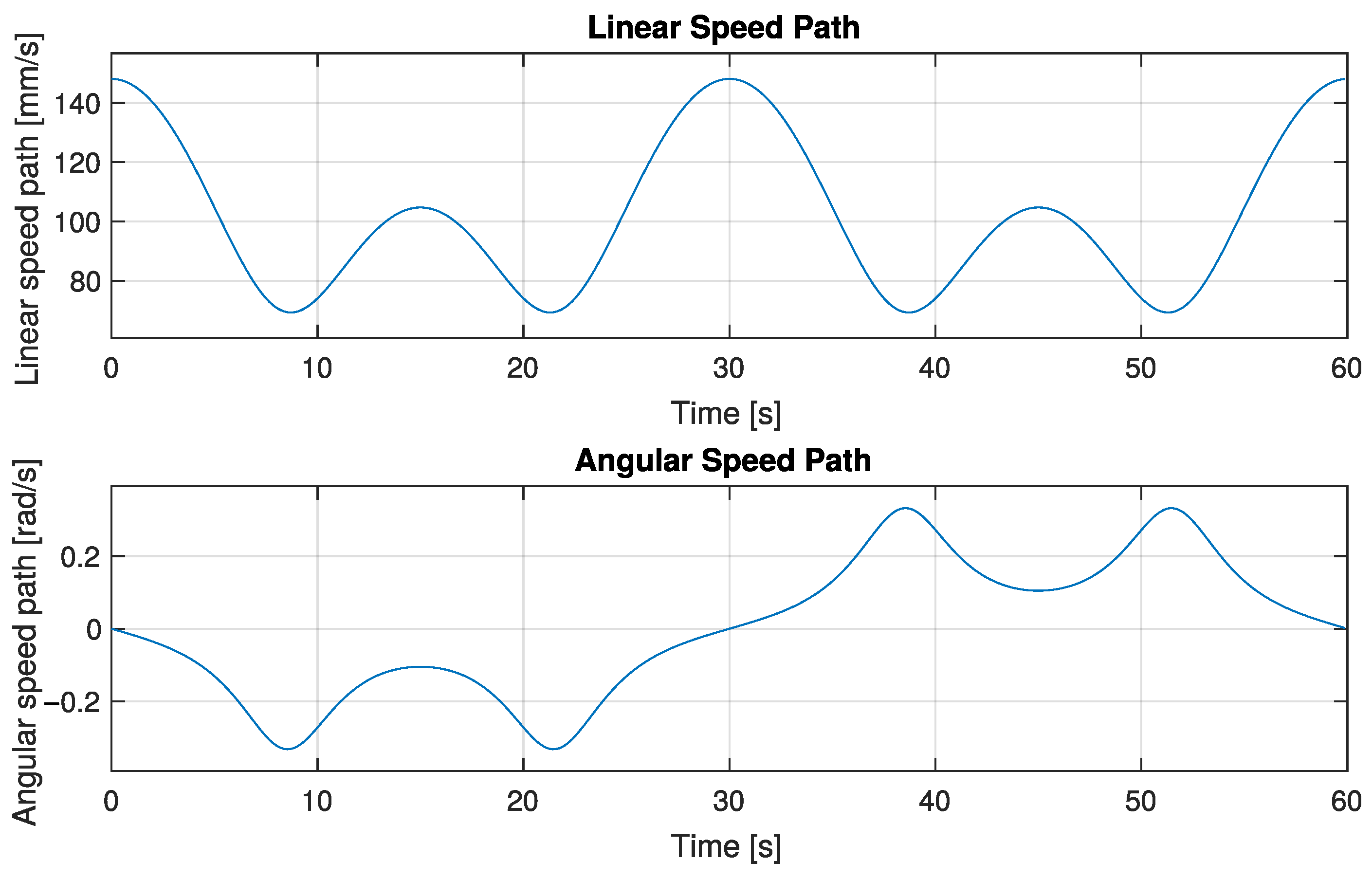
Figure A1 illustrates the behavior of the instantaneous linear and angular velocities along the generated trajectory. In this scenario, the system encounters a trajectory with variable angular and linear velocities.
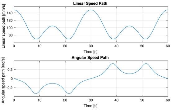
Figure A1.
Instantaneous linear and angular velocity of the generated trajectory.
Figure A1.
Instantaneous linear and angular velocity of the generated trajectory.
References
- Brentari, M.; Zambotti, A.; Zaccarian, L.; Bosetti, P.; Biral, F. Position and speed control of a low-cost two-wheeled, self-balancing inverted pendulum vehicle. In Proceedings of the 2015 IEEE International Conference on Mechatronics (ICM), Nagoya, Japan, 6–8 March 2015; pp. 347–352. [Google Scholar]
- Rahmani, R.; Mobayen, S.; Fekih, A.; Ro, J.S. Robust Passivity Cascade Technique-Based Control Using RBFN Approximators for the Stabilization of a Cart Inverted Pendulum. Mathematics 2021, 9, 1229. [Google Scholar] [CrossRef]
- Valencia-Palomo, G.; Hilton, K.R.; Rossiter, J.A. Predictive control implementation in a PLC using the IEC 1131.3 programming standard. In Proceedings of the 2009 European Control Conference (ECC), Budapest, Hungary, 23–26 August 2009; IEEE: Piscataway, NJ, USA, 2009; pp. 1317–1322. [Google Scholar]
- Valencia-Palomo, G.; Rossiter, J. Novel programmable logic controller implementation of a predictive controller based on Laguerre functions and multiparametric solutions. IET Control Theory Appl. 2012, 6, 1003–1014. [Google Scholar] [CrossRef]
- Diaz, D.; Kelly, R. On modeling and position tracking control of the generalized differential driven wheeled mobile robot. In Proceedings of the 2016 IEEE International Conference on Automatica, ICA-ACCA 2016, Curico, Chile, 19–21 October 2016. [Google Scholar]
- Chan, R.P.M.; Stol, K.A.; Halkyard, C.R. Review of modelling and control of two-wheeled robots. Annu. Rev. Control 2013, 37, 89–103. [Google Scholar] [CrossRef]
- Raudys, A.; Šubonienė, A. A Review of Self-balancing Robot Reinforcement Learning Algorithms. In Proceedings of theCommunications in Computer and Information Science, Curico, Chile, 19–21 October 2020; pp. 159–170. [Google Scholar]
- Kuntal, V.; Kumar, R.; Soni, H.; Sagarmani; Mishra, S.; Singh, S.K.; Choudhury, B. Advancements in Control Algorithms and Key Components for Self-Balancing Electric Unicycles: A Comprehensive Review. In Proceedings of the 2023 3rd International Conference on Innovative Mechanisms for Industry Applications (ICIMIA), Bengaluru, India, 21–23 December 2023; pp. 491–497. [Google Scholar]
- Yue, M.; Wang, S.; Sun, J.Z. Simultaneous balancing and trajectory tracking control for two-wheeled inverted pendulum vehicles: A composite control approach. Neurocomputing 2016, 191, 44–54. [Google Scholar] [CrossRef]
- Chiew, T.H.; Lee, Y.K.; Chang, K.M.; Ong, J.J.; Goh, Y.H. Design and Analysis of Super Twisting Sliding Mode-PID Controller for Two-wheeled Self-balancing Robot. AIP Conf. Proc. 2023, 2680, 020127. [Google Scholar]
- Díaz-Téllez, J.; Gutierrez-Vicente, V.; Estevez-Carreon, J.; Ramírez-Cárdenas, O.D.; García-Ramirez, R.S. Nonlinear Control of a Two-Wheeled Self-balancing Autonomous Mobile Robot. In Advances in Soft Computing, Proceedings of the 20th Mexican International Conference on Artificial Intelligence, MICAI 2021, Mexico City, Mexico, 25–30 October 2021; Springer International Publishing: Cham, Switzerland, 2021; pp. 348–359. [Google Scholar]
- Lower, M. Nonlinear Controller for an Inverted Pendulum Using the Trigonometric Function. Appl. Sci. 2023, 13, 12272. [Google Scholar] [CrossRef]
- Unluturk, A.; Aydogdu, O. Machine Learning Based Self-Balancing and Motion Control of the Underactuated Mobile Inverted Pendulum with Variable Load. IEEE Access 2022, 10, 104706–104718. [Google Scholar] [CrossRef]
- Nougues, S.; Guayacan, S.M.; Cuadros, D.G.; Leon-Rodriguez, H. Modelling and Design a Self-Balancing Dual-Wheeled Robot with PID Control. In Proceedings of the 2023 23rd International Conference on Control, Automation and Systems (ICCAS), Yeosu, Republic of Korea, 17–20 October 2023; pp. 489–497. [Google Scholar]
- Sani, M.A.A.; David, J.B.A.; Jaafar, N.H.; Yusof, M.I.; Sani, N.S.; Sadikan, S.F.N. The Development of a Self-Balancing Robot Based on Complementary Filter and Arduino. In Applied Problems Solved by Information Technology and Software; SpringerBriefs in Applied Sciences and Technology; Springer Nature: Cham, Switzerland, 2024; Part F2025; pp. 71–78. [Google Scholar]
- Bernal, M.; Sala, A.; Lendek, Z.; Guerra, T.M. Analysis and Synthesis of Nonlinear Control Systems; Studies in Systems, Decision and Control; Springer International Publishing: Cham, Switzerland, 2022; Volume 408. [Google Scholar]
- Zhong, W.; Röck, H. Energy and passivity based control of the double inverted pendulum on a cart. In Proceedings of the 2001 IEEE International Conference on Control Applications, Mexico City, Mexico, 7 September 2001; pp. 896–901. [Google Scholar]
- Gómez-Coronel, L.; Alvarado-Algarin, A.; Marquez-Zepeda, M.J.; Ancheyta-López, H.; López-Estrada, F.R.; Santos-Ruiz, I. Modeling and full-state feedback stabilization of a linear inverted pendulum. In Proceedings of the 24th Robotics Mexican Congress, COMRob 2022, Hidalgo, Mexico, 9–11 November 2022; pp. 42–47. [Google Scholar]
- Atoui, H.; Sename, O.; Milanes, V.; Martinez-Molina, J.J. Toward switching/interpolating LPV control: A review. Annu. Rev. Control 2022, 54, 49–67. [Google Scholar] [CrossRef]
- Das, S.; Pan, I.; Halder, K.; Das, S.; Gupta, A. LQR based improved discrete PID controller design via optimum selection of weighting matrices using fractional order integral performance index. Appl. Math. Model. 2013, 37, 4253–4268. [Google Scholar] [CrossRef]
- Duan, G.-R.; Yu, H.H. LMIs in Control Systems: Analysis, Design and Applications; CRC Press: Boca Raton, FL, USA, 2013; pp. 99–102. [Google Scholar]

Disclaimer/Publisher’s Note: The statements, opinions and data contained in all publications are solely those of the individual author(s) and contributor(s) and not of MDPI and/or the editor(s). MDPI and/or the editor(s) disclaim responsibility for any injury to people or property resulting from any ideas, methods, instructions or products referred to in the content. |
© 2024 by the authors. Licensee MDPI, Basel, Switzerland. This article is an open access article distributed under the terms and conditions of the Creative Commons Attribution (CC BY) license (https://creativecommons.org/licenses/by/4.0/).