Analytical Solutions of Microplastic Particles Dispersion Using a Lotka–Volterra Predator–Prey Model with Time-Varying Intraspecies Coefficients

Abstract

Discarded plastic is subjected to weather effects from different ecosystems and becomes microplastic particles. Due to their small size, they have spread across the planet. Their presence in living organisms can have several harmful consequences, such as altering the interaction between prey and predator. Huang et al. successfully modeled this system presenting numerical results of ecological relevance. Here, we have rewritten their equations and solved a set of them analytically, confirming that microplastic particles accumulate faster in predators than in prey and calculating the time values from which it happens. Using these analytical solutions, we have retrieved the Lotka–Volterra predator–prey model with time-varying intraspecific coefficients, allowing us to interpret ecological quantities referring to microplastics dispersion. After validating our equations, we solved analytically particular situations of ecological interest, characterized by extreme effects on predatory performance, and proposed a second-order differential equation as a possible next step to address this model. Our results open space for further refinement in the study of predator–prey models under the effects of microplastic particles, either exploring the second-order equation that we propose or modify the Huang et al. model to reduce the number of parameters, embedding in the time-varying intraspecies coefficients all the adverse effects caused by microplastic particles.

1. Introduction

The discovery of Bakelite in 1907 revolutionized modern life by introducing plastic materials to the world. The popularization of these polymers began with their commercial production around 1950 [1,2]. Plastic’s versatility, stability, low weight, and low production cost leveraged its global market for this material [2]. The increase in plastic consumption has had serious repercussions on nature. It is estimated that 9.5 million tons of plastic end up in the oceans every year [3,4] and there are still no estimates for the amount of plastic deposited on land [5].

All discarded plastic is subject to weather effects of different ecosystems. This material can be slowly degraded by photo-oxidation, thermal pathways, mechanochemical interactions or biodegradation [6]. The results of all these processes are small particles known as microplastics, which have dimensions that vary between 1 μm and 5 mm [7] and the most different compositions, colors, and shapes [8].

Due to their small size, microplastics have spread across the planet. They have already been detected in all parts of the ocean [9], in the poles [10], in drinking water [11], in arable areas and pastures [12], in the habitat of terrestrial animals [13,14,15], and in various foods consumed by people [16]. Many studies suggest that the near-ubiquity of microplastics means that their transfer is not limited to food chain related dynamics, but also occurs through bioaccumulation from one trophic level to another [17,18,19].

The presence of microplastics in living organisms can have several consequences. Studies indicate the possibility of gastrointestinal inflammation [20], decreased reproductive capacity [21], reduced ability to feed [22], reduced growth rate [23], and even malformation of embryos [24]. Early research suggests that microplastics can alter the interaction between prey and predator [25], producing interesting study approaches that use Lotka–Volterra prey–predator models modified to take into account the microplastics [26].

The Lotka–Volterra model (LVM) was originally developed from the logistic equation, describing chemical reactions [27]. However, over the years, modifications of this model have allowed new and specific applications, such as the study of the interaction between prey and predators [28,29,30], the influence of harmful elements on population dynamics [31], and, more specifically, the effect that microplastics has on trophic relationships [18,19,26].

This paper aims to go beyond the numerical solutions of a prey–predator model by studying analytical solutions of the model proposed by Huang et al. [26], which takes into account the impact of microplastics on the population dynamics. We rewrite the Huang et al. four equations model, reducing it to two equations equivalent to one and including the time-varying intraspecies coefficients. This approach clarifies the model parameters meanings and allows us to solve analytically three special cases of ecological relationships. These special cases are based on possible extreme effects of predatory performance reduction caused by exposure to MP particles and are mathematically characterized by the decoupling of the differential equations of the model, for which we also perform numerical simulations. We also propose a second-order differential equation as a possible next step to address this model.

We organized the presentation as follows: In Section 2, we introduce Huang et al.’s work, including their model and main results. In addition, we justify our interest in their research, presenting our motivations and intentions, and rewrite four original equations of the predator–prey model, reducing them to only two ones, redefining/regrouping some quantities, including time-varying intraspecies coefficients, giving them ecological meanings analogous to the standard LVM. In Section 3, we analytically validate that microplastic (MP) particles accumulate faster in predators than in preys and calculate the characteristics times from which their concentration and changing rate of the total amount are greater in predators than in preys. After validating our model, we explore analytically and numerically three special ecological regimes characterized by extreme effects on predatory performance, which can lead these two populations to become independent. In addition, we introduce a second-order differential equation as a possible future study of our two equations system. In Section 4, we compile our results and interpretations, presenting their implications and research possibilities of refining LVM under effects of MP particles, exploring our second-order equation or modifying the standard model to reduce its number of parameters, embedding in the time varying intraspecies coefficients all the adverse effects caused by MP particles. In Section 5, we summarize our main results and point to future studies.

2. Materials and Methods

In 2020, Huang et al. [26] published a study using the LVM where they theoretically investigated predator–prey population dynamics in terms of toxicological response intensity to microplastic (MP) parts and examined the negative effects on prey feeding ability and predator performance due to MP particles. The study suggests that dynamic LVMs can be an important tool to predict the ecological impacts of MP particles on predator–prey population dynamics.

Combining a single-species model with the LVM, Huang et al. obtained the following model:

$$\begin{array}{c}\hfill \left\{\begin{array}{c}{\dot{x}}_1\left(t\right)=x_1\left(t\right)[r_{10}-d_1-r_{11}{C}_1\left(t\right)-(a_1-d_3)x_2\left(t\right)]\hfill \\ {\dot{x}}_2\left(t\right)=x_2\left(t\right)[-r_{20}-r_{21}{C}_2\left(t\right)+(a_2-d_2)x_1\left(t\right)]\hfill \\ {\dot{C}}_1\left(t\right)=S_1{C}_E-g_1\hfill \\ {\dot{C}}_2\left(t\right)=S_2{C}_E+k{C}_1\left(t\right)-g_2\hfill \end{array}\right.,\end{array}$$

(1)

where $x_1\left(t\right),x_2\left(t\right),C_1\left(t\right),C_2\left(t\right)\ge 0$. This model neglects the influence of the intraspecific competition and shows the effect of the microplastics by its concentration. Considering $t\ge 0$ in those differential equations, $x_1$ and $x_2$ represent the population of prey and predator, respectively. $r_{10}{x}_1$ and $r_{20}{x}_2$ are the intrinsic growth rate of prey and mortality rate of predator without toxicity, respectively. $a_1{x}_1{x}_2$ is the lost amount of prey eaten by predators, and $a_2{x}_1{x}_2$ is the increasing number of predators due to the feeding of prey, with $a_1,a_2>0$. The parameters $d_1$, $d_2$, and $d_3$ represent the decline in the prey feeding ability, the adverse effect of reduced predatory performance, and the lost amount of prey eaten by the predator, respectively. The response intensities of MP particles on prey and predator are denoted by $r_{11}$ and $r_{21}$, respectively. The microplastics egestion rates of prey and predator, $g_1,g_2\ge 0$ ($g_1<0$ or $g_2<0$ would imply a MP particles “negative egestion”, by prey or predator), are independent of the microplastics concentration in the environment $C_E\ge 0$, and the amount of microplastics concentration removed at each time step is independent of the total amount of microplastics in the organisms, $C_1$ and $C_2$. The quantity $k{C}_1$ represents the accumulated toxicity of MP particles transferred from the prey. Finally, $S_1,S_2\ge 0$ are related to the effects of plastic particle selection of prey and predator, respectively ($S_1<0$ or $S_2<0$, which would imply an environment MP particle “negative ingestion” rate by prey or predator).

The authors estimated parameters and performed simulations that indicated that predators are more vulnerable than prey under exposure to microplastics. The effect of MP particles on both population growths can be negligible when toxicological response intensities of prey and predator are small, the system is prey-dependent for predator functional response, and the reduced feeding capacity of prey and predator induced by microplastics does not significantly affect the population dynamics. The conclusions are compatible with empirical evidence. This study indicates that this model is adequate to approach the prediction of population dynamics of the predator–prey system under toxicological effects of persistent organic pollutants.

Stimulated by the relevance of the study and the innovativeness of its approach, we decided to explore the Huang et al. model, going beyond its numerical solutions by obtaining analytical solutions that reproduce some of their results, using these solutions to validate our equations, and going even further presenting and analyzing particular cases of possible ecological interest.

After elaborating the model, Huang et al. estimated its parameters and performed numerical simulations, implementing them using MATLAB programming and its Simulink toolbox, based on differential equations such as those presented by the system (1). We have realized that it is possible to rewrite only two equations, reducing them to the derivatives ${\dot{x}}_1\left(t\right)$ and ${\dot{x}}_2\left(t\right)$. In addition, it is interesting to redefine/regroup some quantities of the model, significantly reducing its number of parameters and clarifying its understanding and ecological interpretation. Since some of the parameters in the system are related, we can regroup them into effective (net) and variable rates of decline and growth.

Initially, we define the quantities: $\alpha =a_1-d_3$, which is the difference between the rate of prey population decline and the rate of the lost amount of prey eaten by predators (that we call effective rate of prey population decline), and ${\alpha }^{\prime }=d_2-a_2$, which is the difference between the rate of reduced predatory performance and the rate of predator population growth (that we call negative of the effective rate of predator population growth), and rewrite the system (1):

$$\begin{array}{c}\hfill \left\{\begin{array}{c}{\dot{x}}_1\left(t\right)=x_1\left(t\right)[r_{10}-d_1-r_{11}{C}_1\left(t\right)-\alpha x_2\left(t\right)]\hfill \\ {\dot{x}}_2\left(t\right)=x_2\left(t\right)[-r_{20}-r_{21}{C}_2\left(t\right)-{\alpha }^{\prime }{x}_1\left(t\right)]\hfill \\ {\dot{C}}_1\left(t\right)=S_1{C}_E-g_1\hfill \\ {\dot{C}}_2\left(t\right)=S_2{C}_E+k{C}_1\left(t\right)-g_2\hfill \end{array}\right.,\end{array}$$

(2)

where $x_1\left(t\right),x_2\left(t\right),C_1\left(t\right),C_2\left(t\right)\ge 0$.

We see that the solution to $C_1\left(t\right)$ is a first degree polynomial:

$$C_1\left(t\right)=C_1\left(0\right)+{\tilde{C}}_{1}t,$$

(3)

with

$${\tilde{C}}_1=S_1{C}_E-g_1,$$

(4)

which means that the total amount of microplastics in the prey population varies at a constant rate ${\tilde{C}}_1$. Note that the parameters $S_1$, $C_E$, and $g_1$ combine to form a quantity with units of $\left[C_1\right]/\left[t\right]$.

Using the solution of $C_1\left(t\right)$, we obtain the solution of $C_2\left(t\right)$, which is a second degree polynomial:

$$C_2\left(t\right)=C_2\left(0\right)+{\tilde{C}}_{2}t+\frac{k{\tilde{C}}_1}{2}{t}^2,$$

(5)

with

$${\tilde{C}}_2=S_2{C}_E-g_2+k{C}_1\left(0\right),$$

(6)

meaning that the total amount of microplastics in the predator population, unlike the prey population, varies at a rate that is directly proportional to time, and equal to ${\tilde{C}}_2+k{\tilde{C}}_{1}t$.

Comparing the expressions for the total amount of MP particles in the prey, $C_1\left(t\right)$, and predators, $C_2\left(t\right)$, we show that, over time, the concentration of microplastics inside the predator population will eventually be larger than the concentration inside prey population, which occurs at

$$t_{C_2>C_1}>\frac{\left(\widetilde{C_1}-\widetilde{C_2}\right)+\sqrt{{\left(\widetilde{C_1}-\widetilde{C_2}\right)}^2-2k\widetilde{C_1}\left(C_2\left(0\right)-C_1\left(0\right)\right)}}{k\widetilde{C_1}}.$$

(7)

This result analytically confirms the already known fact [26] that MP particles tend to accumulate faster in predators than in prey, which occurs when the rate of change of the total amount of microplastics inside predators is greater than the rate of change of the total amount of microplastics inside prey, more specifically at

$$t_{\dot{C_2}>\dot{C_1}}>\frac{\widetilde{C_1}-\widetilde{C_2}}{k\widetilde{C_1}}.$$

(8)

Replacing $C_1\left(t\right)$ and $C_2\left(t\right)$ in the first two equations of the system (2), one needs only two coupled differential equations to write the Huang et al. model:

$$\begin{array}{c}\hfill \left\{\begin{array}{c}{\dot{x}}_1\left(t\right)=x_1\left(t\right)\{r_{10}-d_1-r_{11}[C_1\left(0\right)+{\tilde{C}}_{1}t]-\alpha x_2\left(t\right)\}\hfill \\ {\dot{x}}_2\left(t\right)=x_2\left(t\right)\left\{-r_{20}-r_{21}\left[C_2\left(0\right)+{\tilde{C}}_{2}t+\frac{k{\tilde{C}}_1}{2}{t}^2\right]-{\alpha }^{\prime }{x}_1\left(t\right)\right\}\hfill \end{array}\right..\end{array}$$

(9)

Regrouping further this system of equations, one sees that it is possible to rearrange some of its quantities, to obtain variable rates of growth/decline of prey/predators. Regrouping the quantities: $c_0=r_{10}-d_1-r_{11}{C}_1\left(0\right)$, $c_0^{\prime }=-r_{20}-r_{21}{C}_2\left(0\right)$, $c_1=r_{11}{\tilde{C}}_1$, $c_1^{\prime }=r_{21}{\tilde{C}}_2$, and $c_2^{\prime }=r_{21}k{\tilde{C}}_1/2$, we define ${\beta }_1\left(t\right)=c_0-c_{1}t$, which is the rate of prey population growth, and ${\beta }_2\left(t\right)=c_0^{\prime }-c_1^{\prime }t-c_2^{\prime }{t}^2$, which is the rate of predator population decline. Note that the effect of the initial conditions appears only on the coefficients $c_0$ and $c_0^{\prime }$.

In this way, for ${\dot{x}}_i\left(t\right)$, we have:

$$\begin{array}{c}\hfill \left\{\begin{array}{c}{\dot{x}}_1\left(t\right)=x_1\left(t\right)[{\beta }_1\left(t\right)-\alpha x_2\left(t\right)]\hfill \\ {\dot{x}}_2\left(t\right)=x_2\left(t\right)[{\beta }_2\left(t\right)-{\alpha }^{\prime }{x}_1\left(t\right)]\hfill \end{array}\right..\end{array}$$

(10)

This system is similar to the well-known standard Lotka–Volterra (predator–prey) equations, except that its prey population growth and predator population decline rates are now time-varying intraspecific coefficients, which have built-in the effects of microplastics in the organisms.

A simple steady-state analysis ${\dot{x}}_1\left(t\right)={\dot{x}}_1\left(t\right)=0$, as $t\to \infty$, leads to the observed regimes. In one hand, if $x_1(\infty )=0$, then $x_2(\infty )\ge 0$ may have arbitrary values. On the other hand, if $x_2(\infty )=0$, then $x_1(\infty )\ge 0$ may have arbitrary values. In case $x_1(\infty )\ne 0$, then $x_2(\infty )={\beta }_2(\infty )/\alpha \to \infty$. Similarly, $x_2(\infty )\ne 0$, then $x_1(\infty )={\beta }_1(\infty )/\alpha \to \infty$. Particular cases presented below show these asymptotic values.

Huang et al. investigate the toxicological effects of MP particles according to the value of response intensity $r_{11}$ and $r_{12}$ implementing the model (1) using MATLAB programming and its Simulink toolbox. The authors classified interactions into four different conditions (response intensities of prey and predator to toxicological effects induced by MP particles): (a) without the influence of MP particles ($C_1=C_2=r_{11}=r_{21}=0$); (b) predator and prey have the same response strength to MP particles ($\Delta =r_{11}/r_{21}=1.0$); (c) predator has much larger response strength than prey ($\Delta =r_{11}/r_{21}=0.1$); (d) predator has much smaller response strength than prey ($\Delta =r_{11}/r_{21}=10.0$). Huang et al. constructed phase-portraits and short-term population dynamics graphs of predator–prey for each of these four conditions, with the following values: $C_E=30$, $x_1\left(0\right)=100$, $x_2\left(0\right)=100$, $C_1\left(0\right)=0$, $C_2\left(0\right)=0$, $r_{10}=4.1$, $r_{20}=4.0$, $d_1=0.1$, $d_2=0.002$, $d_3=0.002$, $a_1=0.052$, $a_2=0.052$, $g_1=1.2$, $g_2=1.3$, $S_1=0.042$, $S_2=0.039$, $a_1=0.052$, $k=2.0$. In addition, they analyzed the negative effects of PM particles on prey feeding ability and predatory performance increasing the values of $d_1$, $d_2$, and $d_3$ to $d_1=0.6$, $d_2=0.012$, and $d_3=0.012$, and taking three conditions of different response strength ($r_{11}=r_{21}=10.0$; $r_{11}=1.0$; and $r_{21}=10.0$; and $r_{11}=10.0$ and $r_{21}=1.0$).

3. Results

Implementing the model of Equation (10) using the SciPy Python library, with the function odeint from Scipy.integrate package, and considering the five scenarios described in the previous section, we successfully reproduced the phase-portraits and the population dynamics graphs of Huang et al. The system we built consists of only two first-order coupled equations, has a reduced and more comprehensible set of parameters, and reproduces all the results of Huang et al. These equations are decoupled in three situations: $\alpha ={\alpha }^{\prime }=0$, $\alpha =0$, and ${\alpha }^{\prime }=0$, which address specific ecological regimes [32].

3.1. Maximum Reduction of Predatory Performance: $\alpha =0$ and ${\alpha }^{\prime }=0$

Exposure to MP particles can cause anomalous behaviors that impair the prey feeding ability and predatory performance of organisms, which lead, for example, to a decrease in the intrinsic growth rate of prey and a reduction in the number of predators. The Huang et al. model considers some of these harmful effects. For example, it denotes $d_2$ to the adverse effect of reduced predatory performance, and $d_3$ to the consequent lost amount of prey eaten by the predator. In our study, we initially considered the extreme situation in which: 1—the presence of MP particles impairs the predatory performance to the point where there is no further increase in the predators population due to their prey feeding or, in other words, $d_2$ is large enough to reduce to zero the effective rate of predator population growth ($-{\alpha }^{\prime }=a_2-d_2=0$); and 2—as a consequence of the drastic reduction in the predatory performance, no more prey is eaten by predators; in other words, $d_3$ is large enough to reduce to zero the effective rate of prey population decline ($\alpha =a_1-d_3=0$). This is a very special scenario, where the harm caused by microplastics on predators makes these two populations independent, transforming a relationship of predation into a relationship of neutralism, in a process described by the decoupling of the equations for $\dot{x_1}$ and $\dot{x_2}$.

Assuming $\alpha ={\alpha }^{\prime }=0$, the system (10) becomes:

$$\begin{array}{c}\hfill \left\{\begin{array}{c}{\dot{x}}_1\left(t\right)=x_1\left(t\right){\beta }_1\left(t\right)\hfill \\ {\dot{x}}_2\left(t\right)=x_2\left(t\right){\beta }_2\left(t\right)\hfill \end{array}\right.,\end{array}$$

(11)

which describes the population dynamics of two independent groups, prey, and predators, i.e., the variation in the number of individuals in one group does not affect the growth dynamics of the other.

Solving the system above, we get independent solutions for $x_1$ and $x_2$, which will be labeled $\left(ind\right)$ for future reference:

$$x_1^{\left(ind\right)}\left(t\right)=x_1\left(t\right)=x_1\left(0\right)e^{{\int }_0^{t}d{t}^{\prime }{\beta }_1\left(t^{\prime }\right)}=x_1\left(0\right)e^{c_{0}t-c_1{t}^2/2}$$

(12)

and

$$x_2^{\left(ind\right)}\left(t\right)=x_2\left(t\right)=x_2\left(0\right)e^{{\int }_0^{t}d{t}^{\prime }{\beta }_2\left(t^{\prime }\right)}=x_2\left(0\right)e^{c_0^{\prime }t-c_1^{\prime }{t}^2/2+c_2^{\prime }{t}^3/3}.$$

(13)

Analyzing the Equations (12) and (13), it is convenient to calculate $X_1^{\left(ind\right)}\left(t\right)$ and $X_2^{\left(ind\right)}\left(t\right)$:

$$\begin{array}{cc}\hfill X_1^{\left(ind\right)}\left(t\right)& ={\int }_0^{t}d{t}^{\prime }{x}_1^{\left(ind\right)}\left(t^{\prime }\right)\hfill \\ & =x_1\left(0\right)\sqrt{\frac{\pi }{2c_1}}{e}^{\frac{c_0^2}{2c_1}}\left[\mathrm{erf}\left(\frac{c_{1}t-c_0}{\sqrt{2c_1}}\right)-\mathrm{erf}\left(\frac{-c_0}{\sqrt{2c_1}}\right)\right],\hfill \end{array}$$

(14)

$$\begin{array}{cc}\hfill X_2^{\left(ind\right)}\left(t\right)& ={\int }_0^{t}d{t}^{\prime }{x}_2^{\left(ind\right)}\left(t^{\prime }\right)\hfill \\ & =x_2\left(0\right){\int }_0^{t}d{t}^{\prime }{e}^{c_0^{\prime }{t}^{\prime }-c_1^{\prime }{t}^{\prime 2}/2-c_2^{\prime }{t}^{\prime 3}/3},\hfill \end{array}$$

(15)

where the error function is $\mathrm{erf}\left(x\right)=\frac{2}{\sqrt{\pi }}{\int }_0^{x}dt{e}^{-t^2}$.

To calculate $X_1^{\left(ind\right)}\left(t\right)$, we used: $\int dt{e}^{at-b{t}^2}=\frac{\sqrt{\pi }{e}^{\frac{a^2}{4b}}}{2\sqrt{b}}\mathrm{erf}\left(\frac{2bt-a}{2\sqrt{b}}\right)$.

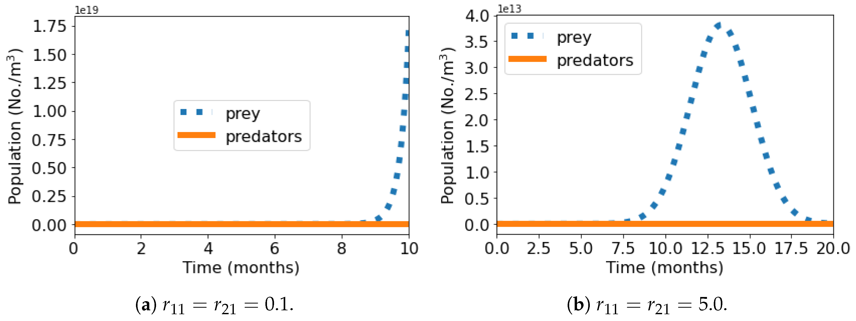
The model (11) was implemented using Python. We performed simulations taking the same scenarios adopted by Huang et al. and described in Section 3. Figure 1 shows the short-term population dynamics graphs of the predator–prey system—the number of organisms (No./m³) versus time (months)—where we observe two patterns: 1—the growth of the prey population at a rate ${\beta }_1\left(t\right)$ accompanied by the extinction of predators and 2—the extinction of both species.

As an example of the first pattern observed when $\alpha ={\alpha }^{\prime }=0$, we consider the case where effects of MP particles on prey and predator are weak ($r_{11}=r_{21}=0.1$). Since prey and predator are independent species and, according to the result of Huang et al., predators are more vulnerable than prey to the effects of MP particles, we have the growth of prey at a rate ${\beta }_1\left(t\right)$ accompanied by the expected extinction of predators (Figure 1a). This behavior was observed in two other scenarios: without the influence of MP particles ($C_1=C_2=r_{11}=r_{21}=0$) and when predators have much larger response strength than prey to MP particles ($r_{11}=0.01$ and $r_{21}=0.1$), in which the effects of microplastics are not strong enough to stop the growth of the prey population. When the response intensities of MP particles on prey and predator are both increased to $r_{11}=r_{21}=5.0$, we have an example of the second pattern, in which the effects of microplastics lead both species to extinction (Figure 1b). Prey population growth is substantially affected by this increase of $r_{11}$, and the number of prey rises at $t=7.5$, peaks at $t=13.7$, and decreases to zero. All other simulated scenarios depict this complete extinction. In these cases, the increase of the adverse effect of reduced predatory performance ($d_2$) and the consequent lost amount of prey eaten by the predator ($d_3$) led to an increasingly early extinction of prey, characterized by curves with increasingly less pronounced peaks.

3.2. Reduction of Predatory Performance with No Prey Eaten by Predator: α = 0

Setting $\alpha =0$ leads to the second case where the equations of the system (10) decouple. In this way, we have

$$\begin{array}{c}\hfill \left\{\begin{array}{c}{\dot{x}}_1\left(t\right)=x_1\left(t\right){\beta }_1\left(t\right)\hfill \\ {\dot{x}}_2\left(t\right)=x_2\left(t\right)[{\beta }_2\left(t\right)-{\alpha }^{\prime }{x}_1\left(t\right)]\hfill \end{array}\right..\end{array}$$

(16)

In the original system (1), since $a_1{x}_1{x}_2$ refers to the lost amount of prey eaten by predators and $d_3{x}_1{x}_2$ refers to the decreasing of that amount, $\alpha =a_1-d_3=0$ describes the regime where the prey population does not decline due to predator feeding (a “total decreasing”).

For $\alpha =0$, the population dynamics of prey are not affected by the predator population size. Nevertheless, the dynamics of predators are affected by the presence of prey. That happens because the model assumes a specific effect that affects the lost amount of prey eaten by predator (denoted by $d_3$) and a distinct effect that affects the number of predators due to their reduced predatory performance (denoted by $d_2$). Thus, even if there is not a lost amount of prey eaten by predators ($\alpha =a_1-d_3=0$), the adverse effect of reduced predatory performance may not be strong enough that the number of predators does not depend on the number of prey (${\alpha }^{\prime }=d_2-a_2$). In this scenario, the effects of microplastics make only the prey population independent.

In this scenario, since $x_1\left(t\right)=x_1^{\left(ind\right)}\left(t\right)=x_1\left(0\right)\exp \left(c_{0}t-c_1{t}^2/2\right)$, we have

$$\begin{array}{ccc}\hfill x_2\left(t\right)& =& x_2\left(0\right)e^{{\int }_0^{t}d{t}^{\prime }[{\beta }_2\left(t^{\prime }\right)-{\alpha }^{\prime }{x}_1^{\left(ind\right)}\left(t^{\prime }\right)]}\hfill \\ & =& x_2^{\left(ind\right)}\left(t\right)e^{-{\alpha }^{\prime }{X}_1^{\left(ind\right)}\left(t\right)},\hfill \end{array}$$

where $x_2^{\left(ind\right)}\left(t\right)=x_2\left(0\right)\exp \left(c_0^{\prime }t-c_1^{\prime }{t}^2/2-c_2^{\prime }{t}^3/3\right)$.

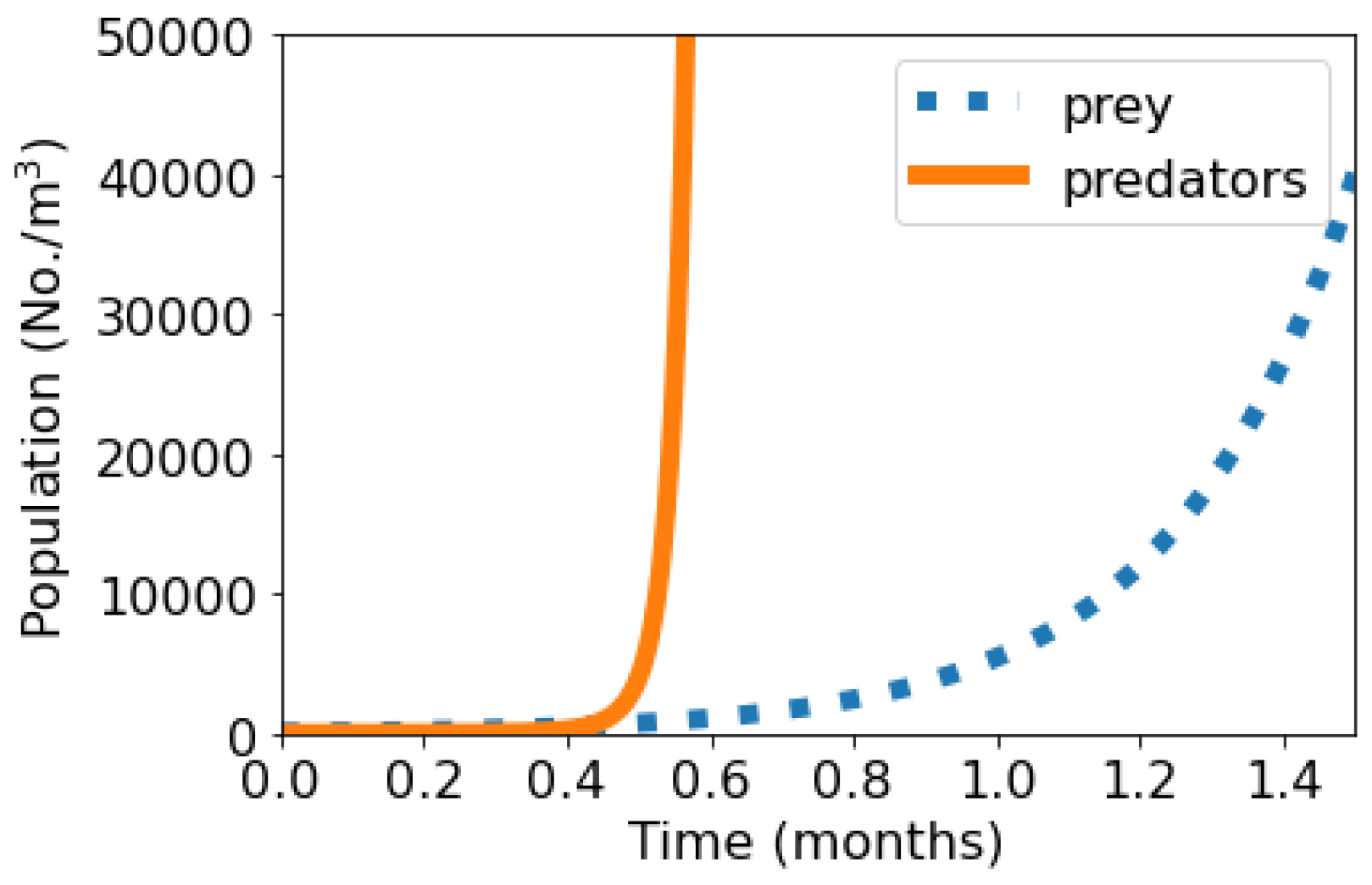
The model (16) was implemented using Python. We performed simulations taking the same scenarios adopted by Huang et al. and described in Section 3. Figure 2 shows the short-term population dynamics graphs of the predator–prey—the number of organisms (No./m³) versus time (months)—where we observe the same pattern, characterized by the growth of the prey population at a rate ${\beta }_1\left(t\right)$ accompanied by the predator “population explosion”.

On one hand, the prey population behaves in these scenarios in the same way as in each of the situations shown in Figure 1, since, in both cases, this population is independent of the predator population and the harmful effects of MP particles are the only factor limiting its growth. On the other hand, the predator population is substantially benefited by its dependence on prey. Figure 2 shows that, in the simulation range allowed by the Python compiler, the number of predators rises very quickly at around $t=0.4$. This “explosive growth” was also observed in all other cases where $\alpha =0$, in which it was noted that it happens at around $t=0.5$ when the values of $d_1$, $d_2$, and $d_3$ are increased.

3.3. Reduction of Predatory Performance with No Increase in the Number of Predators Due to the Feeding of Prey: α′ = 0

A third way to decouple the equations of the system (10) is to make ${\alpha }^{\prime }=0$:

$$\begin{array}{c}\hfill \left\{\begin{array}{c}{\dot{x}}_1\left(t\right)=x_1\left(t\right)[{\beta }_1\left(t\right)-\alpha x_2\left(t\right)]\hfill \\ {\dot{x}}_2\left(t\right)=x_2\left(t\right){\beta }_2\left(t\right)\hfill \end{array}\right..\end{array}$$

(17)

Since $a_2{x}_1{x}_2$ is the increasing number of predators due to the feeding of prey, and $d_2{x}_1{x}_2$ is the decreasing number of predators due to the adverse effect of reduced predatory performance, ${\alpha }^{\prime }=d_2-a_2=0$ defines a regime of reduction of predatory performance, where there is no increase in the number of predators due to the feeding of prey. Here, the exposure to MP particles makes only the predators population independent.

Since $x_2\left(t\right)=x_2^{\left(ind\right)}\left(t\right)=x_2\left(0\right)\exp \left(c_0^{\prime }t-c_1^{\prime }{t}^2/2-c_2^{\prime }{t}^3/3\right)$, we have

$$\begin{array}{ccc}\hfill x_1\left(t\right)& =& x_1\left(0\right)e^{{\int }_0^{t}d{t}^{\prime }{\beta }_1\left(t^{\prime }\right)-\alpha {\int }_0^{t}d{t}^{\prime }{x}_2^{\left(ind\right)}\left(t^{\prime }\right)}\hfill \\ & =& x_1^{\left(ind\right)}\left(t\right)e^{-\alpha X_2^{\left(ind\right)}\left(t\right)}.\hfill \end{array}$$

(18)

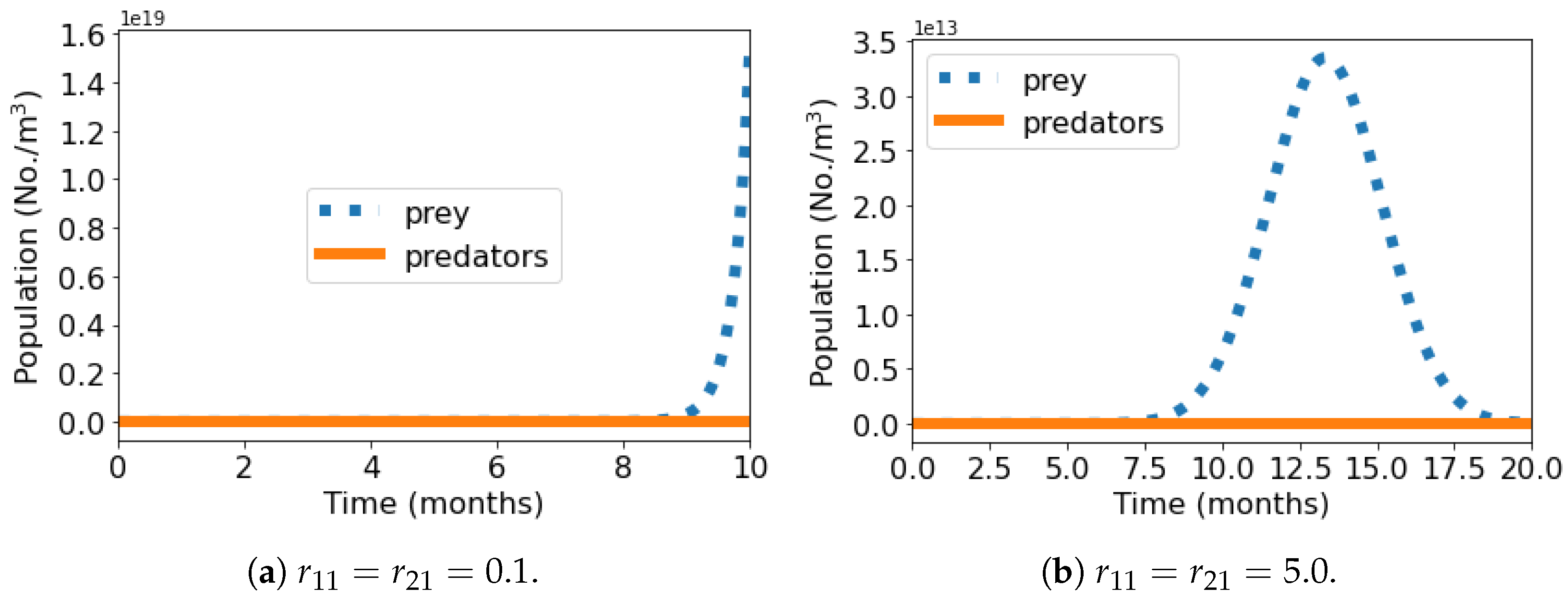
The model (17) was implemented using Python. We performed simulations taking the same scenarios adopted by Huang et al. and described in Section 3. Figure 3 shows the short-term population dynamics graphs of the predator–prey-number of organisms (No./m³) versus time (months)—where we observe the same two patterns of the Section 3.1, where $\alpha ={\alpha }^{\prime }=0$.

When ${\alpha }^{\prime }=0$, the prey population is the only one affected by the presence of the other species, and predator extinction occurs early in every scenario, since there is no increase in its number due to the feeding of the prey, besides being under the harmful effects of the MP particles (Figure 3). Thus, the population dynamics of the system are similar to those in Figure 1. However, it can be seen in each of these situations that the dependence on the predator, even weak, led to an early extinction of the prey, which also presented curves with less pronounced peaks.

A possible next step for a system of ODEs such as (10) is to combine the two first-order differential equations into a single second-order one. To do so, we first write $x_2\left(t\right)$ as a function of ${\beta }_1\left(t\right)$ and the ratio ${\dot{x}}_1/x_1$ and differentiate ${\dot{x}}_1\left(t\right)$ in Equation (10), leading to: ${\ddot{x}}_1\left(t\right)={\dot{x}}_1\left(t\right)[{\beta }_1\left(t\right)-\alpha x_2\left(t\right)]+x_1\left(t\right)[{\dot{\beta }}_1\left(t\right)-\alpha {\dot{x}}_2\left(t\right)]$, and then to: ${\ddot{x}}_1\left(t\right)={\dot{x}}_1\left(t\right){\beta }_1\left(t\right)+x_1\left(t\right){\dot{\beta }}_1\left(t\right)-\alpha \{{\dot{x}}_1\left(t\right)+x_1\left(t\right)[{\beta }_2\left(t\right)-{\alpha }^{\prime }{x}_1\left(t\right)]\}{x}_2\left(t\right)$. Using the calculated $x_2\left(t\right)$, one obtains:

$${\ddot{x}}_1\left(t\right)={\beta }_2{\dot{x}}_1\left(t\right)+\left[{\dot{\beta }}_1\left(t\right)-{\beta }_1\left(t\right){\beta }_2\left(t\right)\right]x_1\left(t\right)+{\alpha }^{\prime }{\beta }_1\left(t\right)x_1^2\left(t\right)-\left[-\frac{{\dot{x}}_1\left(t\right)}{x\left(t\right)}+{\alpha }^{\prime }{x}_1\left(t\right)\right]{\dot{x}}_1\left(t\right),$$

which does not depend on $\alpha$. Analogously, if one had written the second-order equation for $x_2\left(t\right)$, it would be independent of ${\alpha }^{\prime }$. This issue stresses that possibly Huang et al. should be reviewed.

4. Discussion

Rewriting the Huang et al. four equations model, reducing it to a two equations one and including time-varying intraspecies coefficients, allowed us to obtain an equivalent model with a format analogous to the standard LVM. This first step clarified the meanings of the model parameters and led us to explore and solve analytically special, and simpler, cases of ecological relationships. Bioaccumulation of microplastics through food web, and its consequent accelerated accumulation and magnification on predator [17,18,19], is a known effect that we analytically showed based on this model, calculating the time threshold from which their concentration and changing rate of the total amount are greater in predators than in prey.

The three situations that we studied are characterized by some possible behavioral abnormalities caused by the exposure to MP particles. More specifically, we considered effects of reduction of predatory performance [26], where prey is not affected by predator population size ($\alpha =0$), and/or there is no increase in the number of predators due to the feeding of prey (${\alpha }^{\prime }=0$). In our study, theses effects are considered so strong that they can make one of the species independent, or even make both independent of each other. In the cases where $\alpha ={\alpha }^{\prime }=0$ or only ${\alpha }^{\prime }=0$, results reveal basically two patterns, depending on the response strength to MP particles: 1—the growth of prey at a rate ${\beta }_1\left(t\right)$ accompanied by the extinction of predators, where the effects of microplastics are not strong enough to stop the growth of the prey population; and 2—the extinction of predator followed by the eventual extinction of prey. The most interesting, and counterintuitive, result of these three cases appears when $\alpha =0$, where there is predators “population explosion”, showing the predator population is substantially benefited by its dependence on prey. We also point out that the Huang et al. model is not able to address the Allee effect [33,34]. It is important to emphasize that the underlying structure of the model is exponential, and the three special situations that we studied are limit cases, which lead to very different predictions from the original study and result in the extremely large numbers of organisms shown in Figure 1, Figure 2 and Figure 3.

5. Conclusions

We rewrite the Huang et al. model by reducing its number of equations and defining new parameters, making it analogous to the standard LVM with time varying intraspecific coefficients. The time threshold from which the MP particles concentration and changing rate of its total amount are greater in predators than in prey was calculated. We solved analytically specific and simpler ecological situations where the effect of MP particles cause severe abnormal behavior on predator and prey, leading them to become independent of each other. Our simulations reveal a counterintuitive result when toxicological effects of MP particles cause a total interruption of prey feeding ability, which can produce a predator “population explosion”.

Our advance in the analytical treatment of the Huang et al. model opens space for further refinement in the study of predator–prey models under toxicological effects of MP particles, either exploring the second-order equation that we propose or modifying the original model to further reduce its number of parameters, embedding in the time-varying intraspecies coefficients all the adverse effects caused by MP particles.