Article

An Efficient Numerical Scheme Based on Radial Basis Functions and a Hybrid Quasi-Newton Method for a Nonlinear Shape Optimization Problem

Laboratory of Applied Mathematics and Computer Science, Faculty of Science and Technology, Cady Ayyad University, Avenue Abdelkrim El Khattabi B. P., Marrakesh 549, Morocco
*
Author to whom correspondence should be addressed.
Math. Comput. Appl. 2022, 27(4), 67; https://doi.org/10.3390/mca27040067
Submission received: 25 June 2022 / Revised: 31 July 2022 / Accepted: 2 August 2022 / Published: 4 August 2022
(This article belongs to the Special Issue Computing and Green Technology)

Abstract

:
The purpose of this work is to construct a robust numerical scheme for a class of nonlinear free boundary identification problems. First, a shape optimization problem is constructed based on a least square functional. Schauder’s fixed point theorem is manipulated to show the existence solution for the state solution. The existence of an optimal solution of the optimization problem is proved. The proposed numerical scheme is based on the Radial Basis Functions method as a discretization approach, the minimization process is a hybrid Differential Evolution heuristic method and the quasi-Newton method. At the end we establish some numerical examples to show the validity of the theoretical results and robustness of the proposed scheme.

1. Introduction

The aim of this paper is to study a shape optimization problem derived from a class of nonlinear inverse problems, which can describe, for example, chemical reactive flows, nonlinear heat conduction, climate modeling [1,2].
Let us consider the following class of nonlinear inverse problem: find ( Γ , u ) such that
( A ( x , u ) u ) = f in Ω ( A ( x , u ) u ) · ν + β u = g 1 on Σ ( A ( x , u ) u ) · ν = g 2 on Γ u = j on Ω
where Ω is an open-bounded set in R 2 with Ω = Γ Σ , the boundary part Γ is assumed to be unknown (Figure 1). f , g 1 , g 2 , j and β are given functions. The quasilinear term A ( x , t ) is a Caratheodory function assumed to be uniformly elliptic, bounded matrix field and satisfying some weak Lipschitz continuity-type conditions [3]. Since we are dealing with a nonlinear problem, Schauder’s fixed point theorem is recommended for such a situation. To prove the uniqueness we will follow the same steps as in [3].
In the last few years, nonlinear inverse problems have motivated countless scientific works in twop major ways. The first covers theoretical analysis, where several techniques were used such as truncation, Schauder’s fixed point and the topological degree. The second concerns numerical methods: several works proposed different approaches to solve nonlinear inverse problems. In [4], the nonlinear Necrotic cancer model is considered, and the authors prove the existence of an optimal solution, although the numerical approximation is not studied. Zheng and Cui [5] show the existence of an optimal solution of the shape design problem describing cancer growth with the presence of a nonlinear boundary condition. Another approach proposed in [6] focuses on solving the shape design problem that arises in nonlinear axisymmetric magnetostatics using a combined finite element inside the ferromagnetic region, and on exterior air they use the boundary elements. Kolvenbach et al. [7] designed an approach to approximate the solution of a shape optimization problem with a nonlinear PDE-constraint arising in electrical engines and of dynamic elastic structures.
Our contribution aims to establish and show the existence of an optimal solution for the shape optimization problem associated with the inverse problem (1), besides to construct a numerical scheme based on the RBF meshless method as a solver for the state equations. The minimization process will be performed using a hybrid Differential Evolution heuristic method with the BFGS quasi-Newton. Hybrid methods have been lately used to solve several applications in inverse problems. In [8], the authors propose conjugate gradient guided with differential evolution to minimize a shape optimization problem derived from a bilateral free boundaries problem. The same authors, in [9], manipulate the genetic algorithm to find the best initial guess for the conjugate gradient, applied to an optimal control problem of bilateral free boundaries. Mozaffari et al. [10] use the imperialist competitive algorithm with the conjugate gradient combined with the boundary element method for the identification of two interfaces. Another hybridization of the gradient method with the genetic algorithm was proposed in [11] for the computation of a shape cavity in the electrostatic problem.
This choice of RBFs comes from their simplicity to implement and their ability to provide efficient approximation. Compared to one of the most used methods in the literature, the finite element method, RBF methods are accurate, fast, suitable for irregular boundaries and easier to implement than FEM. The disadvantage of RBF methods is the difficulty to control the accuracy of the solution systematically. In contrast with FEM, the error of the approximation became smaller on finer meshes. For RBF methods, increasing the number of nodes may not always lead to more accurate solution. However, a good selection of the shape parameter according to each set of nodes may be the solution to overcame this issue, even if this shape parameter does not have an optimal value known a priori, and several works have proposed some alternatives to find an optimal shape parameter for certain PDEs classes [12,13]. We refer some works that used RBF methods in the approximation of inverse problem [14,15].
To start, let us assume the next parametrization of Γ and Ω ; similarly to [16], we write
Γ ( φ ) = ( x , φ ( x ) ) / x [ a , b ] and Ω ( φ ) = ( x , y ) : y ] 0 , φ ( x ) [ and x ] a , b [ D ,
D is a fixed box in R 2 . Then the set of admissible shapes Π reads
Π = { Ω ( φ ) : φ C 0 ( [ a , b ] ) , H , L > 0 : 0 φ ( x ) H , and φ ( x ) φ ( x ) L x x x , x [ a , b ] } .
Π is equipped with the convergence of characteristic function as a topology. For a given admissible shape Ω Π , we consider the following state equations:
( A ( x , u ) u ) = f in Ω , u = j δ on Ω ,
j δ is noisy data, which satisfy:
j δ j H 1 / 2 ( Ω ) δ .
The other state equation is given as follows
( A ( x , u ) u ) = f in Ω , ( A ( x , u ) u ) · ν + β u = g 1 on Σ , ( A ( x , u ) u ) · ν = g 2 on Γ .
Then, consider the shape functional
J δ ( Ω , u 1 , u 2 ) = 1 2 Ω ( u 1 u 2 ) 2 d x ,
with u 1 and u 2 being the solutions of (2) and (3) respectively.
To this end, the shape optimization problem can be written as follows:
min Ω Π J δ , ρ ( Ω ) : = J δ ( Ω , u 1 , u 2 ) + ρ P ( Ω ) , s . t . u 1 U 1 and u 2 U 2 ,
with ρ > 0 is a penalty coefficient and P ( Ω ) = Ω d s is the regularization term, the space U 1 and U 2 are given by the following
U 1 = u H 1 ( Ω ) , u solution of ( ) , U 2 = u H 1 ( Ω ) , u solution of ( ) .
The rest of this work is organized as follows. In the next section we discuss the existence of an optimal solution to the optimization problem (5). The description of the proposed algorithm is detailed in Section 3. At the end, some numerical illustrations are established in Section 4 to prove the validity of the proposed algorithm.

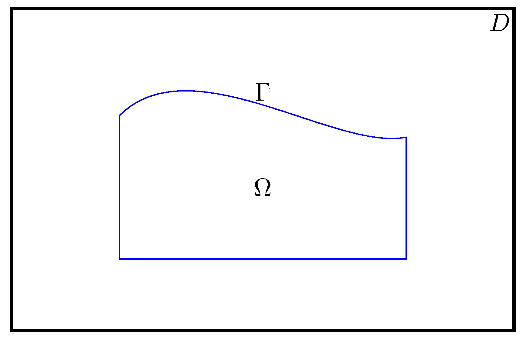
2. Analysis of the Shape Optimization Problem

This section is divided into two parts, in the first one we prove the unique existence of state equation solutions. In the second part we will show the existence of optimal solution of the constrained optimization problem (5).

2.1. Existence of the State Equation Solution

Let η , μ R such that 0 < η < μ , we consider the set
M ( η , μ , D ) = A M 2 ( R ) : ( A ( x ) λ , λ ) η | λ | 2 and | A ( x ) λ | μ | λ | λ R 2 and a . e . D ,
with M 2 ( R ) is the space of 2 × 2 measurable matrix functions.
First we introduce some assumptions to help with the existence of unique solution of the state problems:
H1 
Consider the regularity
1.
f L 2 ( D ) and g 1 , g 2 , j L 2 ( D ) ,
2.
β L ( D ) and there exists C β such that 0 < C β β a.e. in D.
H2 
A is a Caratheodory function, such that:
1.
x A ( x , t ) is measurable for all t R ,
2.
t A ( x , t ) is continuous for almost every x D ,
3.
A ( · , t ) M ( η , μ , D ) for all t R ,
4.
t A ( x , t ) is differentiable for almost every x D .
H3 
There exists a function ϑ : R R that satisfies
1.
ϑ continuous, nondecreasing and non negative function,
2.
| A ( x , ξ 1 ) A ( x , ξ 2 ) | ϑ | ξ 1 ξ 2 | a.e., x D , for ξ 1 ξ 2 ,
3.
for any t > 0 , lim x 0 + x t d ξ ϑ ( ξ ) = + .
Example 1
(function A satisfies assumptions H2 and H3). Consider the nonlinear diffusion function A ( x , u ( x ) ) = exp ( u ( x ) ) , it is obvious that A satisfies the assumptions H2.
Let u and v be two elements of H 1 ( D ) , we write
A ( x , u ( x ) ) A ( x , v ( x ) ) = exp ( u ( x ) ) exp ( v ( x ) ) .
With the mean value inequality theorem applied on the exponential function on the interval
min { u ( x ) , v ( x ) } , max { u ( x ) , v ( x ) } ,
we obtain the existence of a constant C = max x I exp ( x ) > 0 such that
| A ( x , u ( x ) ) A ( x , v ( x ) ) | C | u ( x ) v ( x ) | ,
with
I = ] min { u ( x ) , v ( x ) } , max { u ( x ) , v ( x ) } I ^ = min { u m , v m } , max { u M , v M } [ ,
where u m and u M (resp. v m and v M ) are the min and max values of u (resp. v) on D. Thereafter C C ^ = max x I ^ exp ( x ) , we write then
| A ( x , u ( x ) ) A ( x , v ( x ) ) | ϑ ( | u ( x ) v ( x ) | ) : = C ^ | u ( x ) v ( x ) | ,
which means that ϑ ( ξ ) = C ^ ξ , then ϑ satisfies the assumptionsH3-1andH3-2.
From another hand we have for any t > 0
x t d ξ ϑ ( ξ ) = x t d ξ C ^ ξ = 1 C ^ ln ( t ) ln ( x ) ,
thus
lim x 0 + x t d ξ ϑ ( ξ ) = + .
Let us define the next space:
U = u H 1 ( Ω ) u = j δ on Ω .
Using H1H2, the weak formulation of (2) reads
Find u U such that : for all v H 0 1 ( Ω ) Ω A ( x , u ) u v d x + Σ β u v d s = Ω f v d x .
Similarly we write the weak formulation of (3)
Find u H 1 ( Ω ) such that : for all v H 1 ( Ω ) Ω A ( x , u ) u v d x + Σ β u v d s = Ω f v d x + Σ g 1 v d s + Γ g 2 v d s .
We have the next existence result:
Theorem 1.
For any Ω Π , under assumptionsH1H3, the weak Formulations (6) and (7) admit unique solutions in U and H 1 ( Ω ) , respectively. Moreover, those solutions are bounded independently from Ω.
Proof. 
The proofs of the existence of u 1 and u 2 are quite similar, thus we only concentrate on the existence of u 2 . To establish this proof we will manipulate the Schauder’s fixed point theorem. For that, let us consider the following mapping
T : w L 2 ( Ω ) T ( w ) = u U 2 .
For a fixed w L 2 ( Ω ) we shall prove the solution existence of the next problem
Find u H 1 ( Ω ) such that : for all v H 1 ( Ω ) Ω A ( x , w ) u v d x + Σ β u v d s = Ω f v d x + Σ g 1 v d s + Γ g 2 v d s .
with the fact that A ( x , w ) belongs to M ( η , μ , Ω ) , then there exists a solution of the variational problem (8), we refer the reader to [17].
Now we choose the test function in (8) to be u, and taking into account H2-3 it follows that:
η u 0 , Ω 2 Ω A ( x , w ) | u | 2 d x + Σ β u 2 d s , Ω f u d x + Σ g 1 u d s + Γ g 2 u d s .
With the uniform Poincaré inequality [18], there exists C 0 independent from Ω such that
u 1 , Ω 2 C 0 u 0 , Ω 2 ,
we deduce the estimate
η C 0 u 1 , Ω 2 f 0 , Ω + C 1 g 1 0 , Σ + C 2 g 2 0 , Γ u 1 , Ω .
Thus we obtain
T ( w ) 1 , Ω = u 1 , Ω C 3 with C 3 = C 0 f 0 , D + C 1 g 1 0 , D + C 2 C 2 g 2 0 , D η .
The constant C 2 comes from the continuity of the uniform trace operator [19], in addition it is independent from Ω , which implies that C 3 is also independent from Ω . Now, let the convex set be
W = u L 2 ( Ω ) : u 1 , Ω C 3 .
We ought to show that the mapping T is continuous and compact from W into W. From the definition of W and the estimate (10) we can easily see that T ( W ) W .
Consider then a sequence { w n } from W, we set { u n } = { T ( w n ) } , we have
Ω A ( x , w n ) u n v d x + Σ β u n v d s = Ω f v d x + Σ g 1 v d s + Γ g 2 v d s .
Since { w n } and { u n } are bounded in H 1 ( Ω ) , there exist w and u such that
(i) 
{ u n } converges weakly to u in H 1 ( Ω ) ,
(ii) 
{ w n } converges weakly to w in H 1 ( Ω ) .
By Rellich theorem u n converges strongly to u as a subsequence in L 2 ( Ω ) . Thus { T ( w n ) } is relatively compact, thereafter T is compact.
Now we focus on the continuity of the mapping T. Again with Rellich theorem, there exists a subsequence of { w n } denoted again { w n } , such that
w L 2 ( Ω ) : w n w strong in L 2 ( Ω ) .
To end up the continuity proof we pass to limit in (11), first we mention that
A ( x , w n ) A ( x , w ) a . e in Ω , | A ( x , w n ) v | μ | v | a . e in Ω .
With the Lebesgue dominated convergence theorem we obtain
A ( x , w n ) v A ( x , w ) v a . e . in Ω .
Using the fact that u n converges weakly to u in L 2 ( Ω ) we derive
lim n Ω A ( x , w n ) u n v d x = Ω A ( x , w ) u v d x .
Thereafter we obtain u = T ( w ) , which implies that T is continuous. Hence, Schauder’s fixed point theorem ensures that T admits a fixed point in W.
Now we have proved the solution existence of (3), we move on to show its uniqueness. Consider then u and v two elements of U 2 , we shall show that u = v . Taking the function ϑ in H3-3, following the same manner as in [20] we set
F y ( x ) = y x d t ϑ 2 ( t ) and G y ( x ) = y x d s ϑ ( s ) if x y , F y ( x ) = G y ( x ) = 0 , otherwise .
with y > 0 tending to 0. Moreover, we have the next proprieties [3,20]:
F y ( u v ) , G y ( u v ) H 1 ( Ω ) , X ( u v ) = X ( u v ) ( u v ) with X = F y , G y .
Let us define the set: Ξ = { x Ω : ( u v ) ( x ) > y } . The idea is to show that meas ( Ξ ) = 0 .
Using the fact that u , v U 2 we have
Ω A ( x , u ) u w d x + Σ β u w d s = Ω A ( x , v ) v w d x + Σ β v w d s ,
we choose F y ( u v ) as a test function in the last equation, we obtain:
Ω A ( x , u ) u ( F y ( u v ) ) d x = Ω A ( x , v ) u 2 ( F y ( u v ) ) d x Σ β ( u v ) ( F y ( u v ) ) d s ,
adding the term Ω A ( x , u ) v F y ( u v ) d x with the definition of F y , it follows that
Ξ A ( x , u ) ϑ 2 ( u v ) | ( u v ) | 2 d x = Ξ A ( x , v ) A ( x , u ) ϑ 2 ( u v ) u 2 ( u v ) d x Σ β ( u v ) ( F y ( u v ) ) d s .
Manipulating the assumption H2-3 we obtain
η Ξ 1 ϑ 2 ( u v ) | ( u v ) | 2 d x Ξ A ( x , u ) 1 ϑ 2 ( u v ) | ( u v ) | 2 d x Ξ A ( x , v ) A ( x , u ) 1 ϑ 2 ( u v ) u 2 ( u v ) d x Σ β ( u v ) ( F y ( u v ) ) d s .
The integral Σ β ( u v ) ( F y ( u v ) ) d s is positive, it follows
η Ξ 1 ϑ 2 ( u v ) | ( u v ) | 2 d x Ξ A ( x , v ) A ( x , u ) ϑ 2 ( u v ) u 2 ( u v ) d x .
Taking into consideration H3-2 we deduce
η Ξ 1 ϑ 2 ( u v ) | ( u v ) | 2 d x Ξ 1 ϑ ( u v ) v ( u v ) d x v 0 , Ξ ( u v ) ϑ ( u v ) 0 , Ξ .
Thus
( u v ) ϑ ( u v ) 0 , Ξ C 4 with C 4 = C 3 η .
Using now the function G again, it yields
G y ( u v ) 0 , Ξ C 4 ,
Hence we obtain
G y ( u v ) 1 , Ξ C 5 with C 5 2 = C 4 2 C 0 .
With the results of [20], we have the existence of a sequence { y m } that tends to 0 and a function G H 1 ( Ω ) such that in term of subsequence G y m ( u v ) converges to G weakly in H 1 ( Ω ) and strongly in L 2 ( Ω ) .
Thereafter, lim m + G y m ( u v ) ( x ) < + a.e. in Ω . From the definition of G y and the assumption H3-3 we deduce
lim y m 0 G y m ( u v ) ( x ) = lim y m 0 y m ( u v ) ( x ) d s ϑ ( s ) = + a . e . in Ξ .
Consequently, meas ( Ξ ) = 0 so that u v a.e. in Ω .
To end up the proof we repeat the same technique by changing the roles of u and v which leads to v u , hence the equality.    □
We have proved that there exists a unique solution u 2 of (7) which is bounded by C 3 in H 1 ( Ω ) with C 3 being an independent constant from Ω . Similarly we have the existence of a unique solution u 1 of (6) and there exists C 6 > 0 independent constant from Ω such that u 1 1 , Ω C 6 . We shall highlight that those estimates are held in H 1 ( D ) . If we consider u ˜ denotes the uniform extension of u in H 1 ( D ) [19], from the classical theory we have that u ˜ 1 , D = u 1 , Ω .

2.2. Existence of an Optimal Shape Design

In this part we prove the next existence theorem:
Theorem 2.
The shape optimization problem (5) admits an optimal solution in F .
F = Π × U 1 × U 2 are the feasible solutions spaces of the optimization (5). Before proving this theorem, we need first to define some topology on the space F :
Definition 1.
Consider a sequence { Ω n , u 1 , n , u 2 , n } n = { Ω ( φ n ) , u 1 , n , u 2 , n } n and an element ( Ω , u 1 , u 2 ) b of F . Let’s define the following topology on F :
{ Ω n , u n } n { Ω , u } Ω n n Ω , u 1 , n n u 1 and u 2 , n n u 2 .
The convergence of Ω n to Ω is in the sense of their characteristic functions, u i , n is assumed to converge weakly to u i in H 1 ( Ω ) , which is equivalent to the convergence of their uniform extensions [21] u ˜ i , n to u ˜ i in H 1 ( D ) , for i = 1 , 2 .
Remark 1.
The convergence of Ω n to Ω implies the uniform convergence of φ n and φ n to φ and φ , respectively, in [ a , b ] .
With respect to this topology we have the next compactness result.
Lemma 1.
The space of feasible solutions F is compact.
Proof. 
Let ( Ω n , u 1 , n , u 2 , n ) be a sequence of F , we shall prove the existence of a subsequence of ( Ω n , u 1 , n , u 2 , n ) that converges in F .
First we have Ω n = Ω ( φ n ) , using Ascoli-Arzéla theorem [22] we ensure that ( φ n ) converges uniformly as a subsequence to an element φ , yields Ω = Ω ( φ ) Π .
Since u ˜ i , n are bounded, we can use the Rellich theorem [22] to show the existence of u ˜ i such that u ˜ i , n converges weakly to u ˜ i in H 1 ( D ) . This means that there exists subsequence of { ( Ω n , u 1 , n , u 2 , n ) } that converges to ( Ω , u 1 , u 2 ) , we only need to show that u i U i for i = 1 , 2 . We will only show that u 2 U 2 , to do so we ought to prove that
E ( Ω n , u 2 , n ) n E ( Ω , u 2 )
with
E ( O , ϕ ) , v = O A ( x , ϕ ) ϕ v d x + Σ β ϕ v d s .
We will prove only that
lim n Ω n A ( x , u 2 , n ) u 2 , n v d x = Ω A ( x , u 2 ) u 2 v d x ,
the others term will be shown in a similar way. First we have again
A ( x , u ˜ 2 , n ) A ( x , u ˜ 2 ) a . e in D and u ˜ 2 , n u ˜ 2 weak in L 2 ( D ) .
With the Lebesgue-dominated convergence theorem we infer that
A ( x , u ˜ 2 , n ) u ˜ 2 , n A ( x , u ˜ 2 ) u ˜ 2 weak in L 2 ( D ) .
Now, we write
Ω n A ( x , u 2 , n ) u 2 , n v d x Ω A ( x , u 2 ) u 2 v d x = D χ Ω n χ Ω A ( x , u ˜ 2 , n ) u ˜ 2 , n v d x + D χ Ω n A ( x , u ˜ 2 , n ) u ˜ 2 , n A ( x , u ˜ 2 ) u ˜ 2 v d x .
With the above convergence, it follows that
lim n Ω n A ( x , u 2 , n ) u 2 , n v d x Ω A ( x , u 2 ) u 2 v d x = 0 .
Finally there exists a subsequence of { ( Ω n , u 1 , n , u 2 , n ) } that converges to ( Ω , u 1 , u 2 ) in F , which implies that F is compact.    □
Lemma 2.
The cost functional J δ , ρ is semi lower continuous on F .
Proof. 
Let { ( Ω n , u 1 , n , u 2 , n ) } be a sequence in F that converges to ( Ω , u 1 , u 2 ) in F . With Rellich theorem we have the strong convergence of u ˜ i , n to u ˜ i in L 2 ( D ) as a subsequence for i = 1 , 2 , from another side we have χ Ω n converging to χ Ω in L 1 ( D ) . Thereafter
lim n Ω n u 1 , n u 2 , n 2 d x = lim n D χ Ω n u ˜ 1 , n u ˜ 2 , n 2 d x = Ω u 1 u 2 2 d x .
From another hand, Ω n converges to Ω hence [23]
P ( Ω n ) lim inf n P ( Ω ) .
Finally we obtain
J δ , ρ ( Ω , u 1 , u 2 ) lim inf n J δ , ρ ( Ω n , u 1 , n , u 2 , n ) .
   □
To conclude this section, we shall mention that the proof of Theorem 2 is based on the compactness of the space F and the lower semi-continuity of functional J , which is guaranteed with the last two lemmas.

3. Description of the Proposed Scheme

In this section we concentrate on the description of the proposed scheme to solve the shape optimization problem (5). As mentioned before, the radial basis functions method is chosen to discretize the state equations. For the minimization process, we develop a hybrid method that we split into two phases: the first deals with the use of the differential evolution heuristic method to find a best initial guess, that will be used to run the second phase which concerns the application of the BFGS quasi-Newton.

3.1. RBF Discretization

Consider Ω h a uniform grid of size h of an admissible shape Ω Π
Ω h = { x i c } 1 i N Π h = { Ω ( φ h ) , φ h = ( φ 1 , , φ N ) , 0 φ i H , | φ i + 1 φ i | L h i { 1 , , N 1 } } .
The RBF interpolant writes
u ( x ) = j = 1 N ψ j ( x ) ξ j with ψ j ( x ) = ϕ ε x x j c 2 ,
where · 2 is the Euclidean norm, ϕ is a radial basis function, the coefficient ε is the shape parameters, ξ 1 , , ξ N are the freedom coefficients, they are computed by solving the next matrix system
ϕ ε x 1 x 1 c ϕ ε x 1 x N c ϕ ε x N x 1 c ϕ ε x N x N c ξ 1 ξ N = u 1 u N .
It is known that the RBF interpolation matrix is symmetric, and generally nonsingular which is an issue depending on the choice of the RBF function ϕ ε , in a way to be positive definite. All the choices of RBF given in Table 1 are strictly conditionally positive definite except for the multiquadric RBF, which needs some other arguments to yield a positive definite matrix.
The choice of this parameter affects the accuracy of the interpolation with RBF, such that a bad choice will lead to an ill-conditioned linear system [24]. However, the choice of an optimal shape parameter is one of the delicate problems in RBF approximation; some studies show that it can be done by varying the shape parameter in a range then taking the optimal as the argument with best approximating in error [25]. Others [26] have proposed to take ε = 0.815 d m where d m is the minimum distance between two collocation points. In [13], the choice of a shape parameter is made with respect to the variation of the condition number of the linear system. A few choices of radial basis functions [27] are given in Table 1.
First, we write the state Equations (2) and (3) as
L u i = f in Ω and B i u i = l i on Ω .
where L is the nonlinear operator L = ( A ( x , · ) · ) , B 1 is the identity and B 2 is the mixed Robin and identity mapping, the right-hand sides are l 1 = j δ on Ω , l 2 = g 1 on Σ and g 2 on Γ . Then we can write the following
F 1 ( u 1 ) = 0 and F 2 ( u 2 ) = 0 .
The discrete form of the cost functional is given by the following
J δ , ρ ( Ω h ) = 1 2 M ( Ω h ) ( u 1 u 2 ) , u 1 u 2 + ρ R ( Ω h ) .
with M ( Ω h ) being the mass matrix given by
M ( Ω h ) = Ω h ψ i ( x ) ψ j ( x ) d x i , j .
Then we summarize the optimization problem as next
min Ω h Π h J δ , ρ ( Ω h ) s . t . F 1 ( u 1 ) = 0 and F 2 ( u 2 ) = 0 .
To solve the nonlinear equations F i ( u i ) = 0 we use the nonlinear conjugate gradient method, which is presented below in Algorithm 1.Mca 27 00067 i001

3.2. Computation of the Discrete Gradient

In this part, we will establish the discrete expression of the cost functional gradient. First we write
J δ , ρ ( Ω h ) : = J δ ( Ω h , u 1 ( Ω h ) , u 2 ( Ω h ) ) + ρ R ( Ω h ) .
Then for any admissible direction V we have
J δ , ρ ( Ω h ) ( V ) = ( Ω J δ ( Ω h , u 1 , u 2 ) ) V + ( u 1 J δ ( Ω h , u 1 , u 2 ) ) u 1 ( Ω h ) + ( u 2 J δ ( Ω h , u 1 , u 2 ) ) u 2 ( Ω h ) + R ( Ω h ) V .
Additionally, we have the following
J δ ( Ω h ) = J δ ( Ω ( φ ) ) φ i i = 1 N = 1 2 M ( Ω h ) ( u 1 u 2 ) , u 1 u 2 + M ( Ω h ) ( u 1 u 2 ) , u 1 u 2 ,
where
M ( Ω h ) = M ( Ω ( φ ) ) φ i i = 1 N , u 1 ( Ω h ) = u 1 ( Ω ( φ ) ) φ i i = 1 N and u 2 ( Ω h ) = u 2 ( Ω ( φ ) ) φ i i = 1 N .
Since we have F 1 ( u 1 ) = 0 and F 2 ( u 2 ) = 0 then we can write using the chain rule:
F 1 ( u 1 ) u 1 + F 1 ( u 1 ) u 1 = 0 and F 2 ( u 2 ) u 2 + F 2 ( u 2 ) u 2 = 0 .
The adjoint state solutions can be expressed as next
F 1 ( u 1 ) p 1 = u 1 J δ ( Ω h ) = M ( Ω h ) ( u 1 u 2 ) , F 2 ( u 2 ) p 2 = u 2 J δ ( Ω h ) = M ( Ω h ) ( u 1 u 2 ) .
Thus we have the discrete gradient
J δ , ρ ( Ω h ) = ( Ω J δ ( Ω h ) ) V p 1 F 1 ( u 1 ) u 1 p 2 F 2 ( u 2 ) u 2 + ρ R ( Ω h ) .

3.3. Differential Evolution Heuristic Method

In this part, we put some light on one of the contemporary heuristic methods, the Differential evolution (DE). It was originated by Storn and Price [28]. As in all heuristic methods, DE searches the best solution of an optimization problem by improving a number of candidate solutions until a prescribed stopping criteria is satisfied. Nevertheless, such an optimization method does not guarantee the existence of an optimal solution. Its role in our approach is to search for the best initial guess to initialize the quasi-Newton method, which ensures the existence of an optimal solution in case if it exists.
DE is a population-based method. With an initial population P 0 of M candidate solutions, X i usually called agents. The fitness of X i is equal to the value of the cost functional at X i . Applying three operators mutation, crossover and selection, DE moves a current population to the new future population. It starts by performing the mutation operator, that consists to generate a new agent according to the next:
Y i n + 1 = X k 1 n + ς ( X k 2 n X k 3 n ) for each i { 1 , . . . , M } ,
with n is the current generation number. k 1 , k 2 and k 3 are random indexes generated randomly in { 1 , . . , i 1 , i + 1 , . . M } . The scaling coefficient ς is chosen from [ 0 , 2 ] .
The offspring agent generated by crossover operator is obtained as follows. For each X i P n , generate the new agent
Z i k n + 1 = X i k n if d k > υ Y i k n + 1 if d k υ for each k { 1 , . . . , K } ,
where K is the length of X i , d k is a number chosen randomly in [ 0 , 1 ] for each k, Y i n + 1 is the offspring of the mutation operation (20), υ is the ratio of the crossover.
We come to the last operation, the selection. It is the stage where the decision—which agents will live to the future generation—is made. Based on the fitness of X i n and Z i n + 1 the fittest one will live, meaning the one with the smallest cost value will continue in the future generation P n + 1 .
This choice of this particular heuristic method is due to its efficiency and fast convergence in comparison with the famous heuristic methods used in the literature, such as for example the genetic algorithm, which applies almost the same operators.

3.4. Quasi-Newton Method

Here, we describe a quasi-Newton variant method, the Broyden, Fletcher, Goldfarb and Shanno method (BFGS) [29], which is based on the approximation of Hessian matrix. First, with an initial guess Ω 0 , the iteration is considered:
Ω n + 1 = Ω n + ϱ n d n ,
where ϱ n is the step size, d n is the direction of descent, obtained as solution of the linear system:
L n d n = J δ , ρ ( Ω n ) ,
where L is a matrix updated according to the formula
L n + 1 = L n + Λ n ( Λ n ) T < t n , Λ n > L n [ t n ( t n ) T ] L n < L n t n , t n > ,
L 0 is the identity matrix and
t n = J δ , ρ ( Ω n + 1 ) J δ , ρ ( Ω n ) , and Λ n = Ω n + 1 Ω n .
All the steps of the proposed scheme are summarized in Algorithm 2.Mca 27 00067 i002

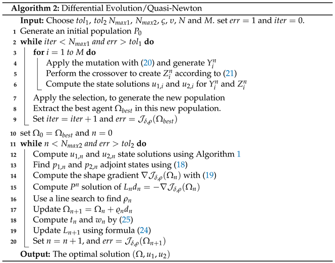
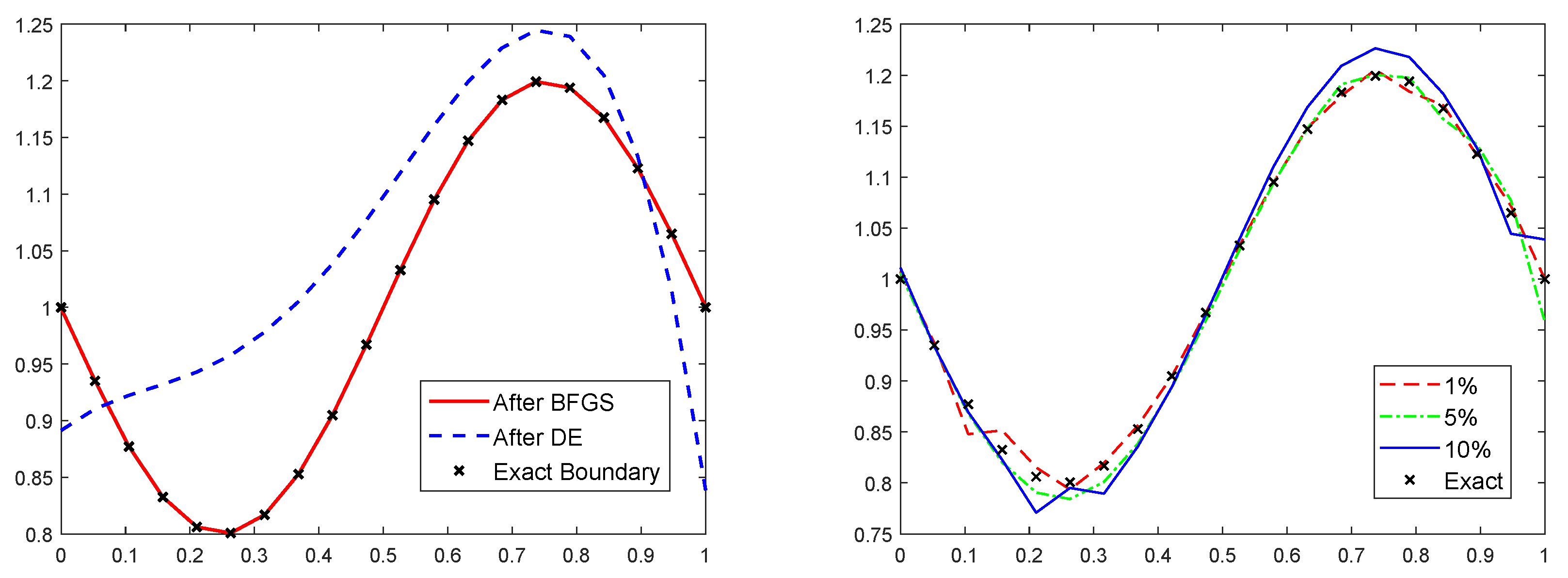
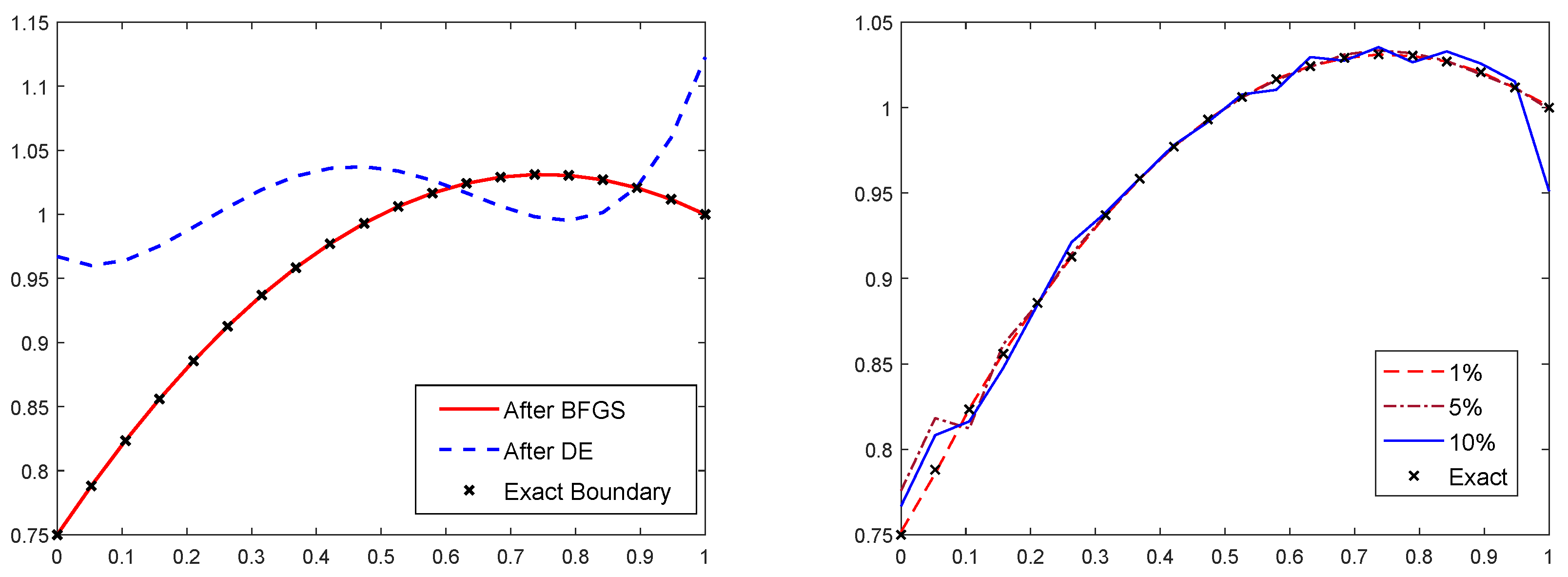
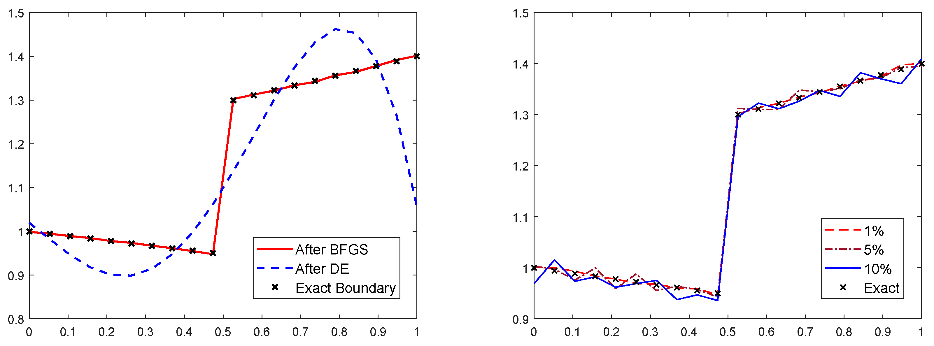
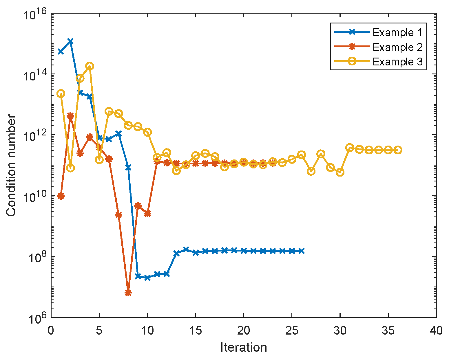
4. Numerical Results

This section is dedicated to establish some numerical experiments to prove from one hand the validity of the theoretical results, the robustness of the proposed numerical scheme from the other hand. All codes are written in MATLAB R2018b. The experiments are run on a laptop of Intel core i5 10th generation 1.60 GHz with 16 GB of RAM. The data in the state problem is constructed with the analytical solution for state Equations (2) and (3) which is given by u e ( x , y ) = 1 x + y + 4 . For the nonlinear operator A we consider the next example A ( x , u ) = e x p ( u ( x ) ) .
In the present study, the inverse multi-quadratic is used as the radial basis function, with a grid of size 20 × 20 . To control the condition number of the linear system, which is influenced by the shape parameter ε , we adapt the approach in [26], where they have proposed that ε = 0.815 d m where d m is the minimum distance between two collocation points. To measure the error for the RBF approximation, we compute the well-known Root Mean Square (RMS) error using:
RMS = 1 N i = 1 N u i z δ 2 .
In the literature, most works take the exact solution in place of z δ ; our consideration comes from the fact that we are dealing with an inverse problem that we seek to solve by controlling the construction of the missing boundary from the given observation only.
Now, we tune the Differential evolution heuristic method. For that, we consider the settings in Table 2.
As described before, after DE achieves the prescribed tolerance or exceeds the maximum of number iterations, its optimal solution is taken as the initial guess for the BFGS algorithm. To tune the BFGS process, we set two criteria, a tolerance t o l 2 = 10 4 and that the difference between two successive iterations Γ n and Γ n + 1 must be smaller than 10 6 .
We test our algorithm for three different types of boundaries Γ i that are characterized by the parametrization φ i , with i = 1 , 2 and 3. The first and the second examples deal with the approximation of the smooth exact boundaries defined by φ i
φ 1 ( x ) = 1 0.2 s i n ( 2 π x ) , and φ 2 ( x ) = 1 + 0.5 ( 1 x ) ( x 0.5 ) , x [ 0 , 1 ] .
For the first and second examples we can easily see in Figure 2 and Figure 3 that the approximated boundary is of relatively good quality. Even with noisy data, the approximated optimal boundary, obtained with the proposed algorithm, is still close enough to the exact boundary. This confirms the efficiency of the proposed approach in approximating such kinds of free boundaries.
The third example has a particularity, we assume that it has a jump in the neighborhood of 0.5 . We consider the function
φ 3 ( x ) = 1.2 0.1 x if x [ 0 , 0.5 ] , φ 3 ( x ) = 1.4 + 0.2 x otherwise .
In Figure 4 we have plotted the obtained results for this last example. Where the DE exceed the 50 iterations without reaching a good precision, the BFGS continued the minimization process; this leads to an accurate approximation of Γ 3 , as shown in the right of Figure 4. When the data became noisy, the solution lost its accuracy, but still delivered an acceptable approximation.
We summarize in Table 3 the optimal RMS error, the final cost and the elapsed time, as well as the total of number of iterations. In Table 4 we record the optimal cost for each example with different noise level. The CPU is very similar for the first and the second examples, but in the third it takes longer due to the complex configuration of the exact boundary; however, the optimal results are of good quality. When the data are noisy, the optimal cost increases with respect to the noise level, although the optimal boundaries are still closer enough to the exact one. Thereupon the proposed scheme is efficient to solve such a nonlinear shape optimization problem.
As we mentioned in the beginning of this section, we seek to control the condition number with adjusting the shape parameter. In Figure 5 we plot the variation of the condition number with respect to the iterations. We easily see that it converges to values less than 10 14 , which means that the approximation is accurate.

5. Conclusions

In this paper, a nonlinear free boundary problem has been considered. The shape optimization technique with regularization was used to write the inverse problem as a constrained optimization problem, and we have shown the existence of its solution. The numerical scheme proposed in this work is the combination of radial basis functions with hybrid Differential evolution and quasi-Newton methods. The shape parameter of the RBF method was controlled with a dynamic formula to ensure that the obtained linear system is well-conditioned. The role of the heuristic differential evolution method was to help with finding the best initial guess for quasi-Newton method. The obtained results show that this hybridization succeeded in achieving an optimal solution with a few iterations. All these results were demonstrated with different numerical examples. At this stage, the proposed scheme is a robust alternative to solve such a nonlinear inverse problem. For future works, we suggest establishing a comparison of the presented scheme based on RBF versus another based on finite element method, and using it in a realistic application.

Author Contributions

Y.E.Y.: Conceptualization, formal analysis, writing—review & editing. A.E.: supervision, review. All authors have read and agreed to the published version of the manuscript.

Funding

This research received no external funding.

Acknowledgments

We are grateful for the insightful comments raised by the anonymous peer reviewers.

Conflicts of Interest

The authors declare no conflict of interest.

References

  1. Cabarrubias, B.; Donato, P. Existence and uniqueness for a quasilinear elliptic problem with nonlinear Robin conditions. Carpathian J. Math. 2011, 27, 173–184. [Google Scholar] [CrossRef]
  2. Conca, C.; Diaz, J.; Linan, A.; Timofte, C. Homogenization in chemical reactive flows. Electron. J. Differ. Equ. 2004, 40, 1–22. [Google Scholar]
  3. Chipot, M. Elliptic Equations: An Introductory Course; Springer Science & Business Media: Berlin/Heidelberg, Germany, 2009. [Google Scholar] [CrossRef]
  4. Wu, J. Analysis of a Nonlinear Necrotic Tumor Model with Two Free Boundaries. J. Dyn. Differ. Equ. 2021, 33, 511–524. [Google Scholar] [CrossRef]
  5. Zheng, J.; Cui, S. Analysis of a tumor model free boundary problem with action of an inhibitor and nonlinear boundary conditions. J. Math. Anal. Appl. 2021, 496, 124793. [Google Scholar] [CrossRef]
  6. Gangl, P.; Langer, U.; Laurain, A.; Meftahi, H.; Sturm, K. Shape Optimization of an Electric Motor Subject to Nonlinear Magnetostatics. SIAM J. Sci. Comput. 2015, 37, B1002–B1025. [Google Scholar] [CrossRef] [Green Version]
  7. Kolvenbach, P.; Lass, O.; Ulbrich, S. An approach for robust PDE-constrained optimization with application to shape optimization of electrical engines and of dynamic elastic structures under uncertainty. Optim. Eng. 2018, 19, 697–731. [Google Scholar] [CrossRef]
  8. El Yazidi, Y.; Ellabib, A. A new hybrid method for shape optimization with application to semiconductor equations. Numer. Algebra Control. Optim. 2021. [Google Scholar] [CrossRef]
  9. El Yazidi, Y.; Ellabib, A. An iterative method for optimal control of bilateral free boundaries problem. Math. Methods Appl. Sci. 2021, 44, 11664–11683. [Google Scholar] [CrossRef]
  10. Mozaffari, M.H.; Khodadad, M.; Dashti Ardakani, M. Simultaneous identification of multi-irregular interfacial boundary configurations in non-homogeneous body using surface displacement measurements. J. Mech. Eng. Sci. 2016, 231, 1–12. [Google Scholar] [CrossRef]
  11. Dashti Ardakani, M.; Khodadad, M. Shape estimation of a cavity by inverse application of the 2D elastostatics problem. Int. J. Comput. Methods 2013, 10, 1350042. [Google Scholar] [CrossRef]
  12. Sanyasiraju, Y.; Satyanarayana, C. On optimization of the RBF shape parameter in a grid-free local scheme for convection dominated problems over non-uniform centers. Appl. Math. Model. 2013, 37, 7245–7272. [Google Scholar] [CrossRef]
  13. Sarra, S. A local radial basis function method for advection-diffusion-reaction equations on complexly shaped domains. Appl. Math. Comput. 2012, 218, 9853–9865. [Google Scholar] [CrossRef] [Green Version]
  14. Jakobsson, S.; Amoignon, O. Mesh deformation using radial basis functions for gradient-based aerodynamic shape optimization. Comput. Fluids 2007, 36, 1119–1136. [Google Scholar] [CrossRef]
  15. Wang, C.; Zhang, J.; Zhou, J. Optimization of a fan-shaped hole to improve film cooling performance by RBF neural network and genetic algorithm. Aerosp. Sci. Technol. 2016, 58, 18–25. [Google Scholar] [CrossRef]
  16. El Yazidi, Y.; Ellabib, A. Augmented Lagrangian approach for a bilateral free boundaries problem. J. Appl. Math. Comput. 2021, 67, 69–88. [Google Scholar] [CrossRef]
  17. Donato, P.; Cioranescu, D.; Zaki, R. Asymptotic behavior of elliptic problems in perforated domains with nonlinear boundary conditions in perforated domains. Asymptot. Anal. 2007, 53, 209–235. [Google Scholar]
  18. Boulkhemair, A.; Chakib, A. On the Uniform Poincaré Inequality. Commun. Partial Differ. Equ. 2007, 32, 1439–1447. [Google Scholar] [CrossRef]
  19. Boulkhemair, A.; Chakib, A.; Nachaoui, A. Uniform trace theorem and application to shape optimization. Appl. Comput. Math. 2008, 7, 192–205. [Google Scholar]
  20. Bendib, S. Homogénéisation dune Classe de Problèmes non Linéaires avec des Conditions de Fourier dans des ouverts Perforés. Ph.D. Thesis, Institut National Polytechnique de Lorraine, Vandœuvre-lès-Nancy, France, 2004. [Google Scholar]
  21. Boulkhemair, A.; Chakib, A.; Nachaoui, A. A shape optimization approach for a class of free boundary problems of Bernoulli type. Appl. Math. 2013, 58, 205–221. [Google Scholar] [CrossRef] [Green Version]
  22. Rudin, W. Functional Analysis; McGraw-Hill: New York, NY, USA, 1991. [Google Scholar]
  23. Zolesio, J.; Sokolowski, J. Introduction to Shape Optimization Shape Sensitivity Analysis; Springer: Berlin/Heidelberg, Germany, 1992. [Google Scholar]
  24. Schaback, R. Error estimates and condition numbers for radial basis function interpolation. Adv. Comput. Math. 1995, 3, 251–264. [Google Scholar] [CrossRef]
  25. Fasshauer, G.; Zhang, J. On choosing “optimal” shape parameters for RBF approximation. Numer. Algorithms 2007, 45, 345–368. [Google Scholar] [CrossRef]
  26. Hardy, R. Multiquadric equations of topography and other irregular surfaces. J. Geophys. Res. 1971, 76, 1905–1915. [Google Scholar] [CrossRef]
  27. Buhmann, M. Radial Basis Functions: Theory and Implementations; Cambridge University Press: Cambridge, UK, 2003; Volume 12. [Google Scholar] [CrossRef]
  28. Storn, R.; Price, K. Differential Evolution—A Simple and Efficient Heuristic for global Optimization over Continuous Spaces. J. Glob. Optim. 1997, 11, 341–359. [Google Scholar] [CrossRef]
  29. Vogel, C. Computational Methods for Inverse Problems; Society for Industrial and Applied Mathematics: Philadelphia, PA, USA, 2002; p. 195. [Google Scholar] [CrossRef]
Figure 1. The geometry of the computational domain.
Mca 27 00067 g001
Figure 2. Results for example 1 without noise (left), with different noise level (right).
Mca 27 00067 g002
Figure 3. Results for example 2 without noise (left), with different noise level (right).
Mca 27 00067 g003
Figure 4. Results for example 3 without noise (left), with different noise level (right).
Mca 27 00067 g004
Figure 5. The condition number with respect to iteration number for each example.
Mca 27 00067 g005
Table 1. Some choices of radial basis function.
NameRBF
Multiquadric (MQ) ϕ ε ( r ) = r ε 2 + 1
Inverse Multiquadric (IMQ) ϕ ε ( r ) = 1 r ε 2 + 1
Gaussian (GA) ϕ ε ( r ) = exp r ε 2
Thin plate spline (TPS) ϕ ε ( r ) = r ε ln ( r ε )
Table 2. Differential evolution parameters.
Population Size tol 1 Max Iterations γ υ
300.5100.050.75
Table 3. Results with exact data.
RMS ErrorCostCPUIterations
Example 1 0.0121 0.0074 225.12 27
Example 2 0.0085 0.0089 281.35 34
Example 3 0.0287 0.0065 372.61 35
Table 4. The optimal cost with noisy data.
Noise LevelExample 1Example 2Example 3
0 % 0.00739 0.00891 0.00655
1 % 0.04079 0.00893 0.01397
5 % 0.06152 0.04258 0.04328
10 % 0.08949 0.05992 0.07012
Publisher’s Note: MDPI stays neutral with regard to jurisdictional claims in published maps and institutional affiliations.

