Abstract
The objective of this paper is to investigate a mathematical model describing the infection of hepatitis B virus (HBV) in intrahepatic and extrahepatic tissues. Additionally, the model includes the effect of the cytotoxic T cell (CTL) immunity, which is described by a linear activation rate by infected cells. The positivity and boundedness of solutions for non-negative initial data are proven, which is consistent with the biological studies. The local stability of the equilibrium is established. In addition to this, the global stability of the disease-free equilibrium and the endemic equilibrium is fulfilled by using appropriate Lyapanov functions. Finally, numerical simulations are performed to support our theoretical findings. It has been revealed that the fractional-order derivatives have no influence on the stability but only on the speed of convergence toward the equilibria.
1. Introduction
The hepatitis B virus (HBV) attacks liver cells (hepatocytes) and kills almost a million people every year. The HBV is known as a global public health issue [1,2], and it infects around two billion people, with more than 360 million chronic carriers. This serious infection can be easily transferred by any infected bodily fluid contact [3,4,5], and it can cause acute or chronic disease following transmission. Many mathematical models have been constructed to represent and better comprehend the dynamics of this deadly viral illness [6,7,8,9]. All of these models take into account how the HBV virus interacts with both healthy and diseased liver cells. However, HBV infection models with two compartments are rare. Recently, the model for describing the adaptive immune response in an HBV infection model with virus to cell transmission in both liver with CTL immune response and the extrahepatic tissue is studied in [10]. They have used the following system of differential equation:
where we denote the liver and the second extrahepatic compartment as compartments and , respectively. In this model, , , , , V and W denote the concentrations of uninfected hepatocytes in , infected hepatocytes in , uninfected hepatocytes in , infected hepatocytes in , free virus and the CTL immune response (in ) at time t, respectively. In addition, is the recruitment rate of healthy cells and is the average lifespan of uninfected cells in compartment . The healthy cells become infected by free virus at a rate , infected cells in compartment die at a rate , and infected cells in compartment are cleared by the CTL immune response at a rate . Free virus (V) grow in blood at a rate , decay at a rate . Finally, CTLs (W) expand in response to viral antigen derived from infected cells at a rate and decay in the absence of antigenic stimulation at a rate .
In this paper, we will study the same above problem but using the fractional derivative equations that will be considered is as follows:
where is the order of the fractional derivative and are the initial data, such as our dynamical model with two HBV proliferative compartments: One is the liver, whereas the other is the extrahepatic compartment, which includes serum, peripheral blood mononuclear cells and perihepatic lymph nodes. According to the investigations, the immune response has an influence, or it has no impact on the extrahepatic compartment. It is considered that the CTL response plays a half function in clearing infected hepatocytes. Furthemore, it has no role in the second proliferative compartment of extrahepatic tissue. We notice that the fractional derivative order can be considered as an index of memory in many biological and physical problems [11]. For instance, for evolution problems in biology, we can find this kind of derivative to model HBV [12]. The fractional derivative equations were used study other models such as Kawahar and KdV equations [13,14,15,16,17]. Different papers studied the behavior of many viral infections by using the fractional derivative equations [18,19,20,21,22]. We notice that the Laplace operator has been used to study the stability of a fractional-order delayed predator–prey system [23]. In addition, fractional derivative have shown its efficiency in studying many biological systems [24,25,26]. Recently, optimal control problems have been studied using fractional derivative equations [27]. These same techniques were applied to study the interaction between tumor cells and the immune system [28]. Therefore, our motivation in this paper is to take into account the memory effect in our biological dynamical system by incorporating the fractional derivative instead of the ordinary one.
The paper is organized as follows. The next section is devoted to the existence, positivity and boundedness of solutions, which is followed in Section 4 by the local stability analysis. In Section 5, we study the global stability of the equilibrium. We construct an appropriate numerical algorithm and give some numerical simulations in Section 6, and the last section concludes the work.
2. Preliminary Results
Is this section, we recall some preliminary definitions of the fractional order integral, Caputo fractional derivative and Mittag–Leffler function [29].
Definition 1.
The fractional integral of order of a function is defined by
where Γ (.) stands for Gamma function.
Definition 2.
The Caputo fractional derivative of order of a function is given as follows
where and . In addition, if , we have
Definition 3.
Let . The function
is called the Mittag–Leffler function of parameter α.
Let where . Consider the fractional order system
with , and . For the global existence of solution of system (2), we have the following lemma.
Lemma 1.
Assume that f satisfies the following conditions
- and are continuous on .
- for all , with and are two positive constants.
Then, the system (2) has a unique solution defind on .
The proof of this lemma follows immediately from [20].
3. Positivity and Boundedness of Solutions
It is commonly known that any solutions reflecting cell densities in issues involving cell population evolution should be non-negative and bounded. As a result, demonstrating the model’s positivity and boundedness will be important. First of all, for biological reasons, the initial data and must be larger than or equal to 0. The main result of this section is given as follows:
Proposition 1.
For any non-negative initial conditions, there exists an unique solution of system (1) defined on . In addition, this solution is non-negative and bounded .
Proof.
Note that if , (3) will be a system with ODEs. By using the results in [19], we establish the existence of solutions. In the case of FDEs, let
and
Therefore,
This implies that
Hence, the proprieties of the previous Lemma are satisfied. Then, system (1) has a unique solution on . Now, we will show that the non-negative solutions : and is positively invariant. Indeed, for , we have:
Therefore, all solutions initiating in are positive. Next, we will prove that these solutions remain bounded.
Therefore, and are bounded.
Therefore, and are bounded.
then
We conclude that all the solutions are bounded and also, each local solution can be prolonged up to any positive time, which means that the solution of the problem exists globally. □
4. Local Stability of Equilibrium
At any equilibrium system, we have
by the first and third equation of this system, we obtain
Substituting them into the second and fourth equations of the same system, they yield, respectively,
We can see that this function is decreasing with respect to V. We have
By the monotonicity of function , Equation (3) has a unique positive root only when
Thus, (1) has a boundary equilibrium when .
When , from the last equation of system (4), we have . Substituting it and into the second equation of (4) gives
Then, a necessary condition on the existence of the positive equilibrium is , and for the positive equilibrium , substituting and into the fifth equation of (4) yields
In the case , we have
Then, according to the monotonicity of function , we have ; then, has a unique root in the interval if and only if . For all this, we will determine the steady states of the model (1). The basic infection reproductive number of the system (1) is given by
From a biological point of view, denotes the average number of secondary infections generated by one infected cell when all cells are uninfected. Moreover, the same system has the following disease-free equilibrium
In addition, model (1) admits two endemic steady states
where
where is the positive root of (4). This endemic equilibrium exists when , and
where
and
Here
and is the positive root of (4). This endemic equilibriam exists when .
5. Global Stability of the Equilibrium
In this section, we will study the global stability of each equilibrium of system (1) by using some suitable Lyapunov functional and by using LaSalle’s invariant principle [4]. For the infection-free equilibrium , we have the following result:
Theorem 1.
If , then the infection-free equilibrium is globally asymptotically stable.
Proof.
When , we have and , that is and . So, is equivalent to the following inequality.
We can choose a positive number satisfying the inequality
then
Furthermore, for the given , we choose a positive number satisfying the inequality
When and are given, we have a Lyapunov function
the derivative of along solutions of our model is given by
Thus, when , then . Let be the largest invariant set in . We observe that if and only if and . Thus, It follows from LaSalle’s invariance principle [8] that the infection-free equilibrium is globally asymptotically stable whenever . □
Theorem 2.
If , then the infection equilibrium is globally asymptotically stable.
Proof.
First, we define a Lyapunov function as follows:
calculating the derivative of along positive solutions of system (4), it follows that
Since the arithmetic mean is greater than or equal to the geometric mean, it follows that
end
Thus, when then Let be the largest invariant set in 0}. We observe that if and only if and . Thus, . Thus, it follows from LaSalle’s invariance principle [8] that the infection-free equilibrium is globally asymptotically stable whenever . □
For the second endemic equilibrium , we have the following result:
Theorem 3.
If and the infection equilibrium of system (1) is globally asymptotically stable.
Proof.
We define first a Lyapunov function as follows:
The derivative of along the positive solutions of the system (1) is
Then
Thus, when and , it implies . Let be the largest invariant set in . We observe that if and only if and for any time t. Therefore, . Since exists whenever , then by the Lyapunov–LaSalle invariance principle [4], is globally asymptotically stable if and . □
6. Numerical Simulations
In the previous sections, we have studied the theoretical part of our fractional problem (1). In this present section, we will present some numerical simulations to the same problem. We notice that the simulation parameters were inspired from [10].
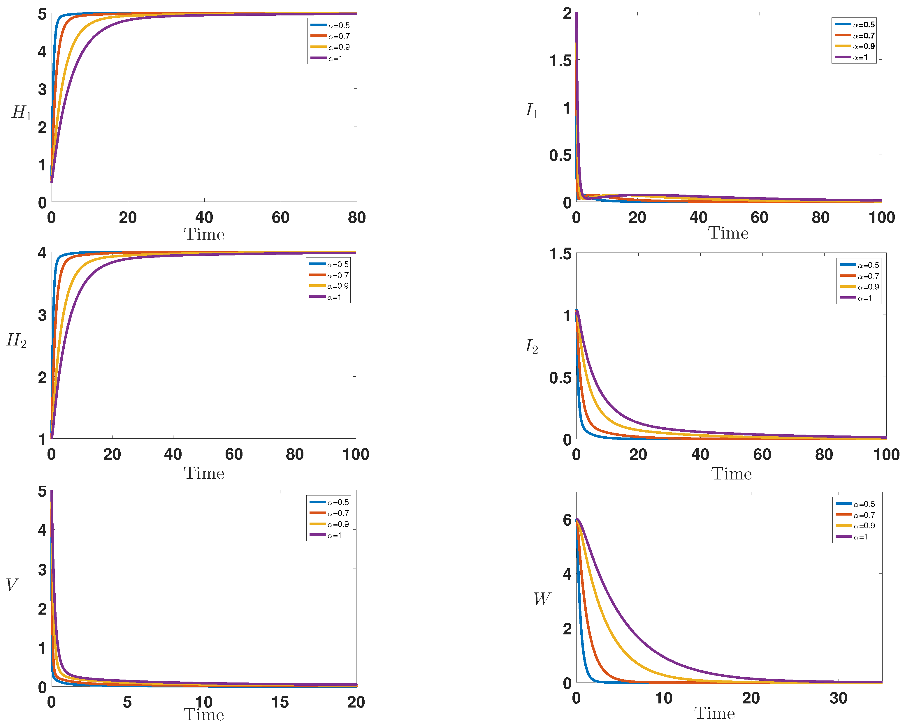
Figure 1 shows the infection dynamics for the following parameters as in the first numerical result of [10]: = 1, = 0.8, = 0.08, = 0.1, = 0.2, = 0.2, = 0.2, = 0.2, = 1, = 1.2, , , = 5 and . Within these chosen parameters, we have that the basic reproduction number is less than unity , and we observe the convergence of the curves, which corresponds to the stability of the disease-free equilibrium . This result is completely is in good agreement with [10] and also confirm our theoretical result given in Theorem 1.
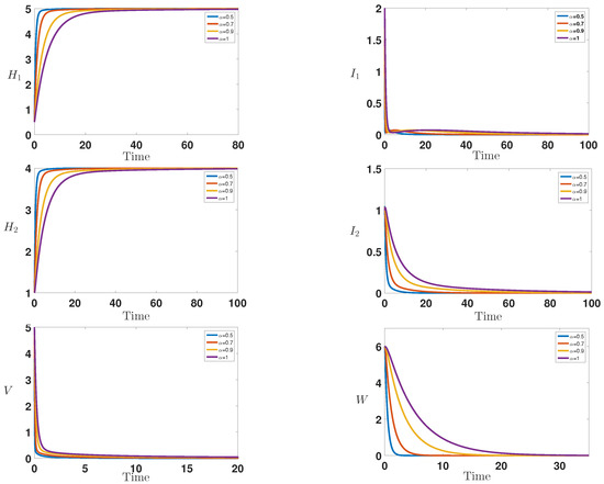
Figure 1.
Behavior of the infection during the time for = 1, = 0.8, = 0.08, = 0.1, = 0.2, = 0.2, = 0.2, = 0.2, = 1, = 1.2, , , = 5 and , which correspond to the stability of the disease-free equilibrium with .
Figure 2 shows the infection dynamics for the following parameters: = 1, = 0.8, = 0.08, = 0.1, = 0.4, = 0.2, = 0.2, = 0.2, = 1, = 1.2, , , = 2.3 and . Within these parameters, we can easily compute the reproduction numbers and , which means that the first one is greater than unity while the second is less than one. This predicts the numerical stability of the first endemic equilibrium . Indeed, we observe that the curves converge toward the first endemic equilibrium , which confirms our theoretical finding concerning the stability of .
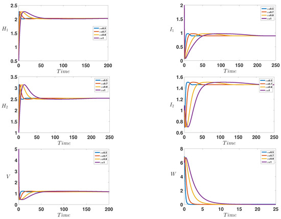
Figure 2.
Behavior of the infection during the time for = 1, = 0.8, = 0.08, = 0.1, = 0.4, = 0.2, = 0.2, = 0.2, = 1, = 1.2, , , = 2.3 and , which correspond to the stability of the endemic equilibrium with and .
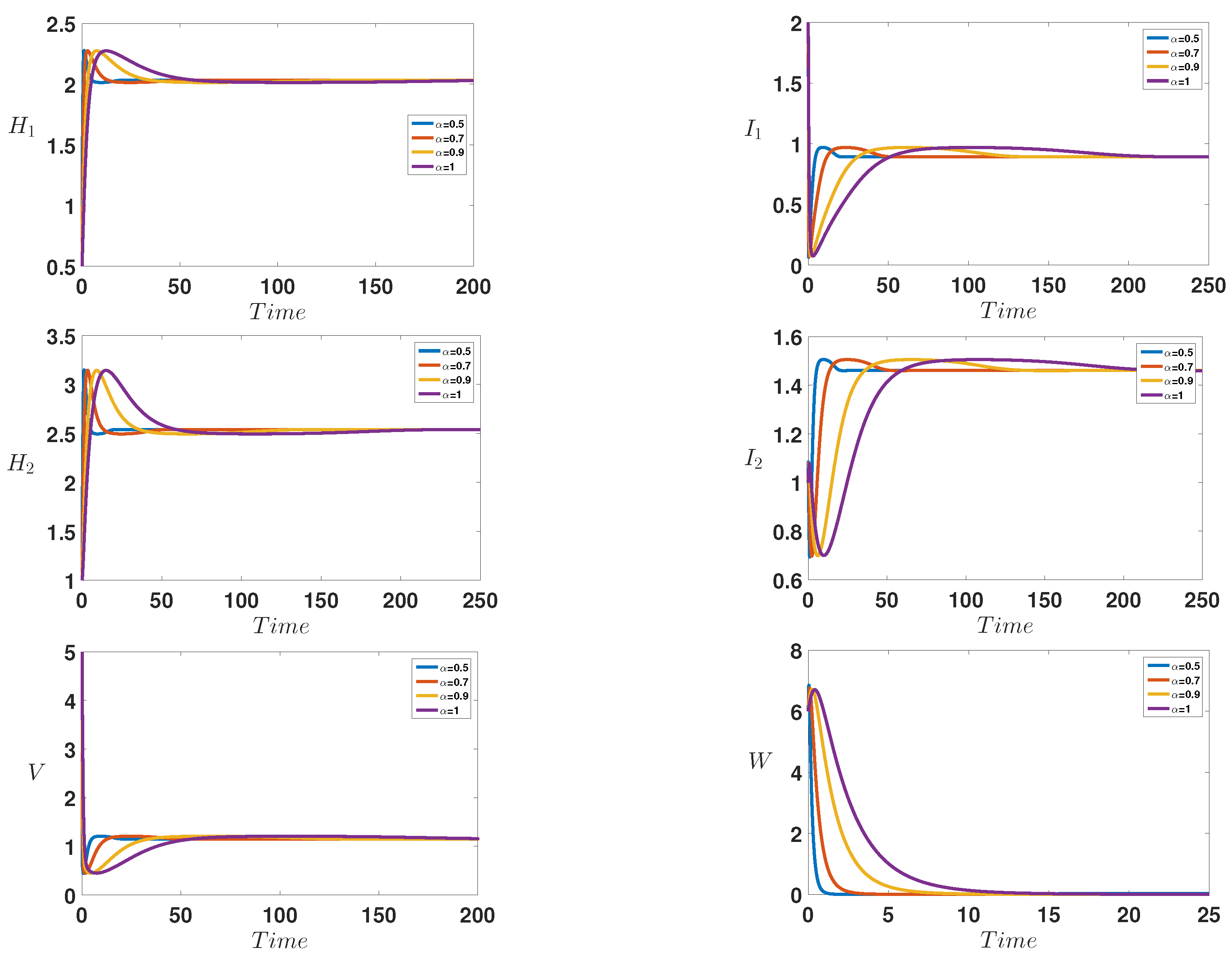
Finally, Figure 3 shows the infection dynamics for the following parameters: , = 0.8, = 0.08, = 0.1, = 0.2, = 0.2, = 0.2, = 0.2, = 1, = 1.2, , , = 2 and . Within these parameters, we can easily compute the reproduction numbers and , which means that both of them are greater than unity. This predicts the numerical stability of the second endemic equilibrium . Indeed, we observe that the curves converge toward the first endemic equilibrium , which confirms our theoretical finding concerning the stability of model (1), which is globally asymptotically stable; this is consistent with Theorem 3.
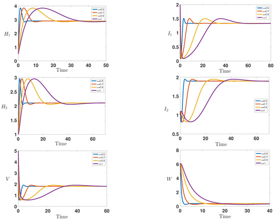
Figure 3.
Behavior of the infection during the time for = 1, = 0.8, = 0.08, = 0.1, = 0.2, = 0.2, = 0.2, = 0.2, = 1, = 1.2, , , = 2 and , which correspond to the stability of the endemic equilibrium ( and ).
7. Conclusions
In this paper, we have studied a mathematical model describing HBV infection in intrahepatic and extrahepatic tissues. In our suggested model, we have taken into consideration the effect of CTL immune response. The positivity and boundedness of solutions for non-negative initial data were proven, which is consistent with the biological background. The local stability of the equilibrium was established. Moreover, the global stability of the disease free equilibrium and the endemic equilibrium was also fulfilled by using some appropriate Lyapanov functional. Numerical tests were performed to support our theoretical findings. In the end of this paper, we have studied the effect of the fractional derivative on the numerical stability of each equilibrium. It has been revealed the fractional order derivative has no influence on the stability but only on the speed of convergence toward the equilibria.
Author Contributions
F.E.F.: Conceptualization, Validation, Formal analysis, Software, Writing—review & editing; K.A.: Conceptualization, Validation, Formal analysis, Software, Writing—review & editing. All authors have read and agreed to the published version of the manuscript.
Funding
This research received no external funding.
Conflicts of Interest
The authors declare no conflict of interest.
References
- Beasley, R.P.; Lin, C.C.; Wang, K.Y.; Hsieh, F.J.; Hwang, L.Y.; Stevens, C.E.; Sun, T.S.; Szmuness, W. Hepatocellular carcinoma and hepatitis B virus. Lancet 1981, 2, 1129–1133. [Google Scholar] [CrossRef]
- World Health Organization Media Centre. 2017. Available online: http://www.who.int/mediacentre/factsheets/fs204/en/ (accessed on 24 June 2022).
- Alter, M.J.; Margolis, H.S.; Krawczynski, K.; Judson, F.N.; Mares, A.; Alexander, W.J.; Hu, P.Y.; Miller, J.K.; Gerber, M.A.; Sampliner, R.E.; et al. The natural history of community-acquired hepatitis C in the United States. N. Engl. J. Med. 1992, 327, 1899–1905. [Google Scholar] [CrossRef] [PubMed]
- LaSalle, J.P. The Stability of Dynamical Systems; SIAM: Philadelphia, PA, USA, 1976. [Google Scholar]
- WHO. Global Hepatitis Report; WHO: Paris, France, 2017. [Google Scholar]
- Zhang, S.; Zhou, Y. The analysis and application of an HBV model. Appl. Math. Model. 2012, 36, 1302–1312. [Google Scholar] [CrossRef]
- Thornley, S.; Bullen, C.; Roberts, M. Hepatitis B in a high prevalence New Zealand population: A mathematical model applied to infection control policy. Nat. Med. 2008, 254, 599–603. [Google Scholar] [CrossRef]
- Pang, J.; Cui, J.; Zhou, X. Dynamical behavior of a hepatitis B virus transmission model with vaccination. Nat. Med. 2010, 265, 572–578. [Google Scholar] [CrossRef] [PubMed]
- Zou, L.; Zhang, W.; Ruan, S. Modeling the transmission dynamics and control of hepatitis B. Nat. Med. 2010, 262, 330–338. [Google Scholar]
- Hu, X.; Li, J.; Feng, X. Threshold dynamics of a HCV model with virus to cell transmission in both liver with CTL immune response and the extrahepatic tissue. J. Biol. Dyn. 2021, 15, 19–34. [Google Scholar] [CrossRef] [PubMed]
- Du, M.; Wang, Z.; Hu, H. Measuring memory with the order of fractional derivative. Sci. Rep. 2013, 3, 3431. [Google Scholar] [CrossRef]
- Danane, J.; Allali, K.; Hammouch, Z. Mathematical analysis of a fractional differential model of HBV infection with antibody immune response. Chaos Solitons Fractals 2020, 136, 109787. [Google Scholar] [CrossRef]
- Bhatter, S.; Mathur, A.; Kumar, D.; Singh, J. A new analysis of fractional Drinfeld–Sokolov–Wilson model with exponential memory. Physica A 2020, 537, 122578. [Google Scholar] [CrossRef]
- Bhatter, S.; Mathur, A.; Kumar, D.; Nisar, K.S.; Singh, J. Fractional modified Kawahara equation with Mittag–Leffler law. Chaos Solitons Fractals 2020, 131, 109508. [Google Scholar] [CrossRef]
- Veeresha, P.; Prakasha, D.G.; Singh, J. Solution for fractional forced KdV equation using fractional natural decomposition method. AIMS Math. 2020, 5, 798–810. [Google Scholar] [CrossRef]
- Boukhouima, A.; Hattaf, K.; Yousfi, N. Dynamics of a fractional order HIV infection model with specific functional response and cure rate. Int. J. Differ. Equ. 2017, 2017, 8372140. [Google Scholar] [CrossRef] [Green Version]
- Ahmed, E.; El-Saka, H.A. On fractional-order models for hepatitis C. Nonlinear Biomed. Phys. 2010, 4, 1. [Google Scholar] [CrossRef] [Green Version]
- Rihan, F.A.; Sheek-Hussein, M.; Tridane, A.; Yafia, R. Dynamics of hepatitis C virus infection: Mathematical modeling and parameter estimation. Math. Model. Nat. Phenom. 2017, 12, 33–47. [Google Scholar] [CrossRef] [Green Version]
- Zhou, X.; Sun, Q. Stability analysis of a fractional-order HBV infection model. Int. J. Adv. Appl. Math. Mech. 2014, 2, 1–6. [Google Scholar]
- Salman, S.M.; Yousef, A.M. On a fractional-order model for HBV infection with cure of infected cells. J. Egypt. Math. Soc. 2017, 25, 445–451. [Google Scholar]
- Yildiz, T.A.; Jajarmi, A.; Yildiz, B.; Baleanu, D. New aspects of time fractional optimal control problems within operators with nonsingular kernel. Discret. Contin. Dyn. Syst. Ser. S 2020, 13, 407. [Google Scholar]
- Baleanu, D.; Jajarmi, A.; Sajjadi, S.S.; Mozyrska, D. A new fractional model and optimal control of a tumor-immune surveillance with non-singular derivative operator. Chaos 2019, 29, 083127. [Google Scholar] [CrossRef] [PubMed]
- Rihan, F.A.; Lakshmanan, S.; Hashish, A.H.; Rakkiyappan, R.; Ahmed, E. Fractional-order delayed predator–prey systems with Holling type-II functional response. Nonlinear Dyn. 2015, 80, 777–789. [Google Scholar] [CrossRef]
- Rihan, F.A.; Arafa, A.A.; Rakkiyappan, R.; Rajivganthi, C.; Xu, Y. Fractional-order delay differential equations for the dynamics of hepatitis C virus infection with IFN-α treatment. Alex. Eng. J. 2021, 60, 4761–4774. [Google Scholar] [CrossRef]
- Rihan, F.A. Numerical modeling of fractional-order biological systems. Abstr. Appl. Anal. 2013, 2013, 816803. [Google Scholar] [CrossRef] [Green Version]
- Rihan, F.A.; Baleanu, D.; Lakshmanan, S.; Rakkiyappan, R. On fractional SIRC model with Salmonella bacterial infection. Abstr. Appl. Anal. 2014, 2014, 136263. [Google Scholar] [CrossRef] [Green Version]
- Delavari, H.; Baleanu, D.; Sadati, J. Stability analysis of Caputo fractional-order nonlinear systems revisited. Nonlinear Dyn. 2012, 67, 2433–2439. [Google Scholar] [CrossRef]
- Magin, R.L. Fractional calculus models of complex dynamics in biological tissues. Comput. Math. Appl. 2010, 59, 1586–1593. [Google Scholar] [CrossRef] [Green Version]
- Podlubny, I. Fractional Differential Equations; Academic Press: San Diego, CA, USA, 1999; p. 198. [Google Scholar]

Publisher’s Note: MDPI stays neutral with regard to jurisdictional claims in published maps and institutional affiliations. |
© 2022 by the authors. Licensee MDPI, Basel, Switzerland. This article is an open access article distributed under the terms and conditions of the Creative Commons Attribution (CC BY) license (https://creativecommons.org/licenses/by/4.0/).