Article

Theoretical and Computational Results of a Memory-Type Swelling Porous-Elastic System

by
Adel M. Al-Mahdi
1,2,*,
Mohammad M. Al-Gharabli
1,2 and
Mohamed Alahyane
3
1
The Preparatory Year Program, King Fahd University of Petroleum and Minerals, Dhahran 31261, Saudi Arabia
2
The Interdisciplinary Research Center in Construction and Building Materials, King Fahd University of Petroleum & Minerals, Dhahran 31261, Saudi Arabia
3
L2EP, Faculty of Sciences and Technologies, University of Lille, 59655 Villeneuve d’Ascq, France
*
Author to whom correspondence should be addressed.
Math. Comput. Appl. 2022, 27(2), 27; https://doi.org/10.3390/mca27020027
Submission received: 22 January 2022 / Revised: 4 March 2022 / Accepted: 7 March 2022 / Published: 11 March 2022

Abstract

:
In this paper, we consider a memory-type swelling porous-elastic system. First, we use the multiplier method to prove explicit and general decay results to solutions of the system with sufficient regularities. These decay results are established under a very general assumption on the relaxation function and for suitable given data. We also perform several numerical tests to illustrate our theoretical decay results. Our results generalize and improve many earlier results in the literature.
JEL Classification:
93D20; 35B40

1. Introduction

There are many different types of clay soils that swell considerably when water is added or absorbed in them and shrink with the loss of the water. This type of soil is termed expansive [1]. When a soil deposit is loaded, for example, by a structure or man-made fill, deformation will occur. Normally, deformation downward is called settlement. Deformation may also be directed upward, which is then called heave. A common cause of heaving is that a building or pavement is constructed when the topsoil layer is relatively dry. Then, the structure covering the soil increases in water content due to capillarity action, and the soil swells.
Heave will result if the pressure exerted by the pavement or building is less than the swelling pressure. The heave is usually uneven and causes structural damage [2]. Documented evidence shows that problems associated with expansive soils are worldwide and occur in areas, such as South Africa, Australia, India, United States, South America, and the Middle East [3]. Swelling soils causes serious engineering problems. Estimates indicate that about 20–25% of land area in the United State is covered with such problematic soils with an accompanied economic loss of 5.5 to 7 billions USD in 2003 [4].
Hence, it is crucial to study the ways to annihilate or at least minimize such damage. The reader is referred to [5,6,7,8,9,10,11,12,13] for other details concerning swelling soil. As established by Ieşan [14] and simplified by Quintanilla [15], the basic field equations for the linear theory of swelling porous elastic soils are mathematically given by
ρ z z t t = P 1 x G 1 + F 1 ρ u u t t = P 2 x + G 2 + F 2 ,
where the constituents z and u represent the displacement of the fluid and the elastic solid material, respectively. The positive constant coefficients ρ z and ρ u are the densities of each constituent. The functions ( P 1 , G 1 , F 1 ) represent the partial tension, internal body forces, and eternal forces acting on the displacement, respectively. Similar definition holds for ( P 2 , G 2 , F 2 ) but acting on the elastic solid. In addition, the constitutive equations of partial tensions are given by
P 1 P 2 = a 1 a 2 a 2 a 3 A z x u x ,
where a 1 , a 3 are positive constants and a 2 0 is a real number. The matrix A is positive definite in the sense that a 1 a 3 a 2 2 . Quintanilla [15] investigated (1) by taking
G 1 = G 2 = ξ ( z t u t ) , F 1 = a 3 z x x t , F 2 = 0 ,
where ξ is a positive coefficient, with initial and homogeneous Dirichlet boundary conditions and obtained an exponential stability result. Similarly, Wang and Guo [16] considered (1) with initial and some mixed boundary conditions, taking
G 1 = G 2 = 0 , F 1 = ρ z γ ( x ) z t , F 2 = 0 ,
where γ ( x ) is an internal viscous damping function with a positive mean. They used the spectral method to establish an exponential stability result. Ramos et al. [17] looked into the following swelling porous elastic soils
ρ z z t t a 1 z x x a 2 u x x = 0 , i n 0 , L × I R + ρ u u t t a 3 u x x a 2 z x x + γ ( t ) g ( u t ) = 0 , i n 0 , L × I R + ,
and established an exponential decay rate provided that the wave speeds of the system are equal. Recently, Apalara [18] considered the following
ρ z z t t a 1 z x x a 2 u x x = 0 , in ( 0 , 1 ) × ( 0 , ) , ρ u u t t a 3 u x x a 2 z x x + 0 t g ( t s ) u x x ( x , s ) d s = 0 , in ( 0 , 1 ) × ( 0 , ) , z ( x , 0 ) = z 0 ( x ) , z t ( x , 0 ) = z 1 ( x ) , u ( x , 0 ) = u 0 ( x ) , u t ( x , 0 ) = u 1 ( x ) , x [ 0 , 1 ] , u ( 0 , t ) = u ( 1 , t ) = z ( 0 , t ) = z ( 1 , t ) = 0 , t 0 ,
where the relaxation function satisfies the condition
g ( t ) ξ ( t ) g ( t ) , t 0
and established a general decay result. For more results in porous elasticity system, porous-thermo-elasticity systems, Timoshenko system and other systems, we refer the reader to see [15,16,19,20,21,22,23,24,25,26,27,28,29,30,31,32,33].
In this paper, we consider the problem (4), where the solution is ( z , u ) such that z and u represent the displacement of the fluid and the elastic solid material. The positive constant coefficients ρ u and ρ z are the densities of each constituent. The coefficients a 1 , a 2 and a 3 are positive constants satisfying specific conditions. We establish a new asymptotic behavior of the above swelling porous elastic system under the condition
g ( t ) ξ ( t ) H g ( t ) , t 0 ,
where ξ and H are two functions that satisfy some conditions to be specified later. Precisely, in our paper:
  • We consider Problem (4) and establish a general decay result with a wider class of relaxation functions than the one considered in the literature such that the one by Apalara [18] is a special case of our class. Our result is obtained by using the multiplier method and some convexity properties.
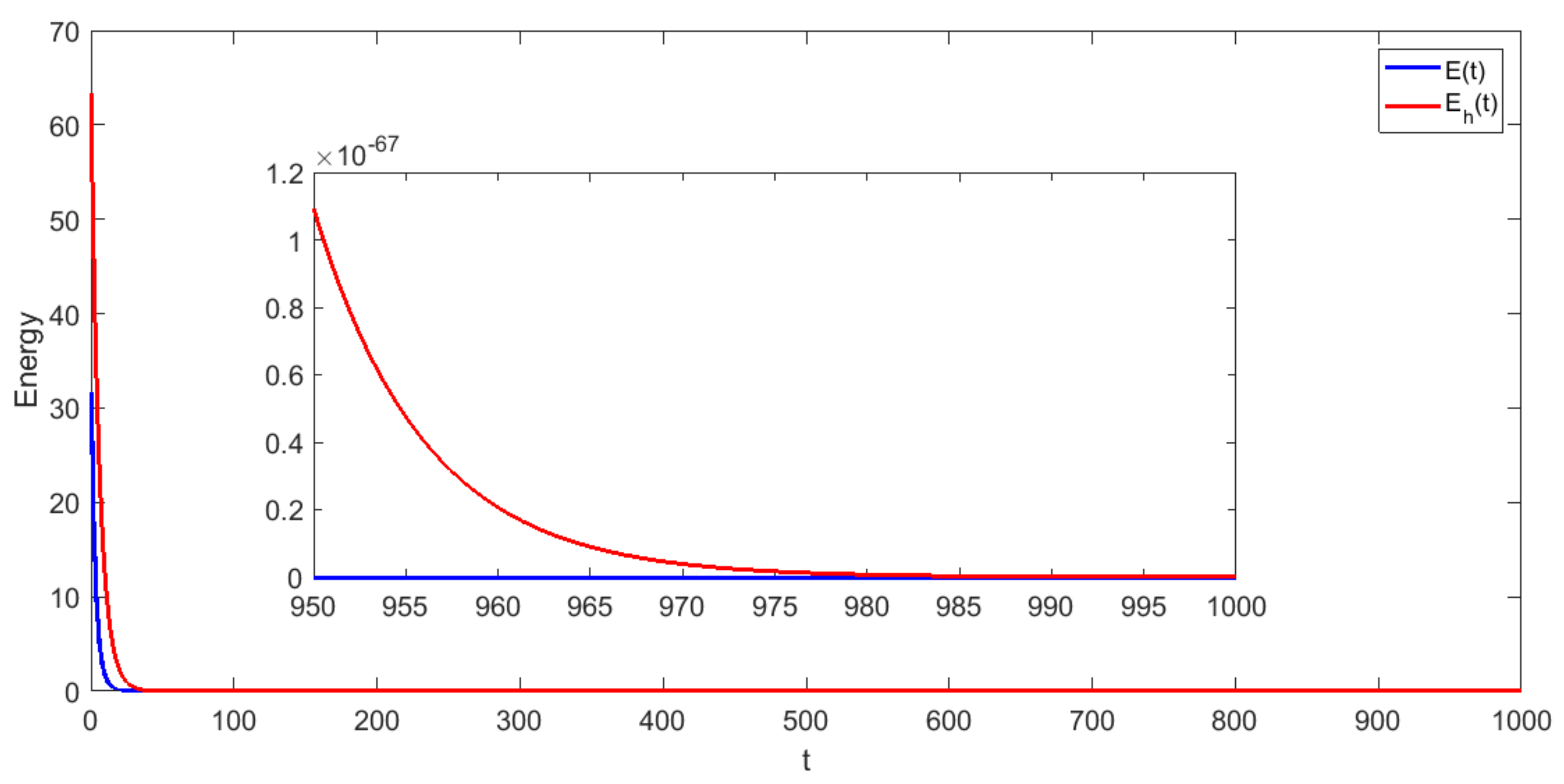
  • We produce some numerical experiments to illustrate the energy decay results, for this purpose, we develop a second-order numerical scheme to solve the problem (4) based on finite element discretization and the Crank–Nicolson method in time that has the property to be unconditionally stable.
  • The result is significant to engineers and architects as it might help to attenuate the harmful effects of swelling soils swiftly.
It is worth mentioning that (6) was first introduced in [34]. The rest of this paper is organized as follows. In Section 2, we present some assumptions and material needed for our work. In Section 3, we state and establish some essential lemmas needed in our proof. Finally, we state and prove our main decay result in Section 4. We also, in Section 5, present some numerical tests to illustrate our decay results as well as our conclusions.

2. Assumptions

In this section, we state some assumptions needed in the proof of our results. Throughout this paper, c is used to denote a generic positive constant. For the relaxation function g, we assume the following:
( A ) g : [ 0 , + ) ( 0 , + ) is a C 1 nonincreasing function satisfying
g ( 0 ) > 0 a n d 0 < : = 0 + g ( s ) d s < a 3 a 2 2 a 1 .
In addition, there exists a C 1 function H : ( 0 , ) ( 0 , ) , which is linear or it is strictly increasing and strictly convex C 2 function on ( 0 , r ] , r g ( 0 ) , with H ( 0 ) = H ( 0 ) = 0 , such that
g ( t ) ξ ( t ) H ( g ( t ) ) , t 0 ,
where ξ is a positive nonincreasing differentiable function.
Remark 1
([35]). If H is a strictly increasing and strictly convex C 2 function on ( 0 , r ] , with H ( 0 ) = H ( 0 ) = 0 , then it has an extension H ¯ , which is a strictly increasing and strictly convex C 2 function on ( 0 , ) . For instance, if H ( r ) = a , H ( r ) = b , H ( r ) = c , we can define H ¯ , for t > r , by
H ¯ = c 2 t 2 + ( b c r ) t + a + c 2 r 2 b r .
Lemma 1.
The energy functional E , is defined by
E ( t ) = 1 2 0 1 ρ z z t 2 + a 1 z x 2 + ρ u u t 2 + a 3 0 t g ( s ) d s u x 2 + 2 a 2 z x u x d x + 1 2 ( g u x ) ( t ) ,
where
( g v ) ( t ) = 0 1 0 t g ( t s ) | v ( t ) v ( s ) | 2 d s d x
satisfies
E ( t ) = 1 2 g u x 1 2 g ( t ) 0 1 u x 2 d x 1 2 ( g u x ) ( t ) 0 .
Proof. 
The routine multiplication of the first two equations of (4) by z t and u t , respectively, and then integrating by parts over ( 0 , 1 ) , leads to
1 2 d d t 0 1 ρ z z t 2 + a 1 z x 2 + ρ u u t 2 + a 3 u x 2 + 2 a 2 z x u x d x 0 1 u x t 0 t g ( t s ) u x ( s ) d s d x = 0 .
The estimation of the second term in the left hand side gives
0 1 u x t 0 t g ( t s ) ( u x ( t ) u x ( s ) ) d s d x 0 t g ( s ) d s 0 1 u x u t x d x = 1 2 d d t g u x 1 2 d d t 0 t g ( s ) d s 0 1 u x 2 d x 1 2 g u x + 1 2 g ( t ) 0 1 u x 2 d x .
Consequently, by substituting (14) into (13), we obtain (12). □

3. Technical Lemmas

In this section, we present and establish some essential lemmas needed for our work.
Lemma 2
([35]). There exist positive constants β 0 and t 1 such that
g ( t ) β 0 g ( t ) , t [ 0 , t 1 ] .
Lemma 3
([35]). For all u H 0 1 ( [ 0 , 1 ] ) ,
0 1 0 t g ( t s ) | u x ( s ) u x ( t ) | d s 2 d x C α ( h u x ) ( t ) ,
for any 0 < α < 1 ,
C α = 0 g 2 ( s ) α g ( s ) g ( s ) d s a n d h ( t ) = α g ( t ) g ( t ) .
It is worth mentioning that the constants C α were first introduced in [36].
Lemma 4.
The functional
F 1 ( t ) : = ρ u 0 1 u t u d x a 2 a 1 ρ z 0 1 z t u d x
satisfies, for any ε 1 > 0 and some constant a 0 ,
F 1 ( t ) a 0 2 0 1 u x 2 d x + ε 1 0 1 z t 2 d x + ρ u + a 2 2 ρ z 2 4 ε 1 a 1 2 0 1 u t 2 d x + C α 2 a 0 ( h u x ) ( t ) ,
where a 0 = a 3 a 2 2 a 1 0 g ( s ) d s > 0 .
Proof. 
Direct computations using integration by parts gives
F 1 ( t ) = a 3 a 2 2 a 1 0 1 u x 2 d x + ρ u 0 1 u t 2 d x a 2 ρ z a 1 0 1 z t u t d x + 0 1 u x 0 t g ( t s ) u x ( s ) d s d x .
Applying Young’s inequalities, we obtain, for ε 1 > 0 ,
a 2 ρ z a 1 0 1 z t u t d x ε 1 0 1 z t 2 d x + a 2 2 ρ z 2 4 ε 1 a 1 2 0 1 u t 2 d x ,
and for ε 2 > 0 ,
0 1 u x 0 t g ( t s ) u x ( s ) d s d x = 0 t g ( s ) d s 0 1 u x 2 d x 0 1 u x 0 t g ( t s ) ( u x ( t ) u x ( s ) ) d s d x 0 t g ( s ) d s + ε 2 2 0 1 u x 2 d x + C α 2 ε 2 ( h u x ) ( t ) .
Combining (19)–(21), we obtain
F 1 ( t ) a 3 a 2 2 a 1 0 g ( s ) d s ε 2 2 0 1 u x 2 d x + ε 1 0 1 z t 2 d x + ρ u + a 2 2 ρ z 2 ε 1 a 1 2 0 1 u t 2 d x + C α 2 ε 2 ( h u x ) ( t ) .
Using assumption ( A ) , taking ε 2 = a 0 , where a 0 = a 3 a 2 2 a 1 0 g ( s ) d s , we obtain (18). □
Lemma 5.
Assume that ( A ) holds. Then, for any t 1 > 0 , the functional
F 2 ( t ) : = ρ u 0 1 u t 0 t g ( t s ) ( u ( t ) u ( s ) ) d s d x
satisfies, for any δ 2 , δ 3 > 0 ,
F 2 ( t ) ρ u c 0 2 0 1 u t 2 d x + δ 1 0 1 u x 2 d x + δ 3 a 2 2 0 1 z x 2 d x + c C α δ 1 + c δ 2 ( 1 + C α ) + C α δ 3 + C α ( h u x ) ( t ) ,
where c 0 = 0 t 1 g ( s ) d s .
Proof. 
Differentiating F 2 , taking into account (4), and using integrating by parts, we obtain
F 2 ( t ) = ρ u 0 t g ( s ) d s 0 1 u t 2 d x + a 3 0 1 u x 0 t g ( t s ) ( u x ( t ) u x ( s ) ) d s d x 0 1 0 t g ( t s ) u x ( s ) d s 0 t g ( t s ) ( u x ( t ) u x ( s ) ) d s d x ρ u 0 1 u t 0 t g ( t s ) ( u ( t ) u ( s ) ) d s d x + a 2 0 1 z x 0 t g ( t s ) ( u x ( t ) u x ( s ) ) d s d x = ρ u 0 t g ( s ) d s 0 1 u t 2 d x + 0 1 0 t g ( t s ) ( u x ( t ) u x ( s ) ) 2 d x + a 3 0 t g ( s ) d s 0 1 u x 0 t g ( t s ) ( u x ( t ) u x ( s ) ) d s d x + a 2 0 1 z x 0 t g ( t s ) ( u x ( t ) u x ( s ) ) d s d x ρ u 0 1 u t 0 t g ( t s ) ( u ( t ) u ( s ) ) d s d x .
Using Young’s inequality and Lemma 3, for any δ 1 > 0 , we obtain
a 3 0 t g ( s ) d s 0 1 u x 0 t g ( t s ) ( u x ( t ) u x ( s ) ) d s d x δ 1 0 1 u x 2 ( t ) d x + c C α δ 1 ( h u x ) ( t ) .
Similarly, we can find, for any δ 2 > 0 ,
ρ u 0 1 u t ( t ) 0 t g ( t s ) ( z ( t ) z ( s ) ) d s d x = ρ u 0 1 u t ( t ) 0 t h ( t s ) ( u ( t ) u ( s ) ) d s d x ρ u 0 t u t ( t ) 0 t α g ( t s ) ( u ( t ) u ( s ) ) d s d x δ 2 0 1 u t 2 ( t ) d x + ρ u 2 0 t h ( s ) d s 2 δ 2 ( h u ) ( t ) + ρ u 2 α 2 2 δ 2 0 1 0 t g ( t s ) ( u ( t ) u ( s ) d s 2 d x δ 2 0 1 u t 2 ( t ) d x + c 2 δ 2 ( h u x ) ( t ) + α 2 c C α 2 δ 2 ( h u x ) ( t ) δ 2 0 1 u t 2 ( t ) d x + c δ 2 ( 1 + C α ) ( h u x ) ( t ) .
Using Young’s inequality and performing similar calculations as in (25), we obtain, for any δ 3 > 0
a 2 0 1 u x 0 t g ( t s ) ( u x ( t ) u x ( s ) ) d s d x δ 3 a 2 2 0 1 u x 2 d x + C α δ 3 ( h u x ) ( t ) .
Employing Lemma 3, we find
0 1 0 t g ( t s ) ( u x ( t ) u x ( s ) ) d s 2 d x C α ( h u x ) ( t ) .
Combining all the above estimates, we find, for any t t 1
F 2 ( t ) ρ u 0 t g ( s ) d s δ 2 0 1 u t 2 d x + δ 2 0 1 u x 2 d x + δ 3 a 2 2 0 1 z x 2 d x + c C α δ 1 + c δ 2 ( 1 + C α ) + C α δ 3 + C α ( h u x ) ( t ) .
By taking δ 2 = ρ u c 0 2 , we obtain the desired inequality (23). □
Lemma 6.
Assume that ( A ) holds. Then, the functional
F 3 ( t ) : = a 2 0 1 u z t z u t d x
satisfies
F 3 ( t ) a 2 2 2 ρ u 0 1 z x 2 d x + a 2 2 ρ z + 3 a 1 2 ρ u + 3 2 ρ u a 1 ρ z a 3 ρ u 2 0 1 u x 2 d x + 3 C α 2 ρ u ( h u x ) ( t ) .
Proof. 
Direct computation gives
F 3 ( t ) = a 2 2 ρ u 0 1 z x 2 d x + a 2 2 ρ z 0 1 u x 2 d x + a 2 a 1 ρ z a 3 ρ u 0 1 u x z x d x a 2 ρ u 0 1 z x 0 t g ( t s ) u x ( s ) d s d x .
Using Young’s inequality, we find
a 2 a 1 ρ z a 3 ρ u 0 1 u x z x d x a 2 2 η 2 2 0 1 z x 2 d x + 1 2 η 2 a 1 ρ z a 3 ρ u 2 0 1 u x 2 d x .
Exploiting Young’s inequality again, we obtain
a 2 ρ u 0 1 z x 0 t g ( t s ) u x ( s ) d s d x = a 2 ρ u 0 1 z x 0 t g ( t s ) u x ( s ) u x ( t ) d s d x + a 2 ρ u 0 t g ( s ) d s 0 1 u x z x d x a 2 2 η 2 2 0 1 z x 2 d x + 1 2 η 2 ρ u 2 0 1 0 t g ( t s ) | u x ( s ) | | u x ( t ) | d s 2 d x + 1 2 η 2 ρ u 2 0 t g ( s ) d s 2 0 1 u x 2 d x + + a 2 2 η 2 2 0 1 z x 2 d x a 2 2 η 2 0 1 z x 2 d x + C α 2 η 2 ρ u 2 ( h u x ) ( t ) + a 1 2 η 2 ρ u 2 0 1 u x 2 d x .
By taking η 2 = 1 3 ρ u and using the fact that 0 t g ( s ) d s a 1 , estimate (29) is established. □
Lemma 7.
The functional
F 4 ( t ) : = ρ z 0 1 z t z d x
satisfies, for any ε 3 > 0 ,
F 4 ( t ) ρ z 0 1 z t 2 d x + a 1 + a 2 2 ε 3 0 1 z x 2 d x + ε 3 0 1 u x 2 d x .
Proof. 
It is straight forward to see that
F 4 ( t ) = ρ z 0 1 z t 2 d x + a 1 0 1 z x 2 d x + a 2 0 1 z x u x d x .
Using Young’s inequality and the fact that a 1 a 3 > a 2 2 , we obtain (31). □
Lemma 8.
Under the assumption ( A ) , the functional
F 5 ( t ) : = Ω 0 t p ( t s ) | u x ( s ) | 2 d s d x
satisfies, along the solution of Equation (4), the estimate
F 5 ( t ) 1 2 ( g u x ) ( t ) + 3 a 1 0 1 u x 2 d x ,
where p ( t ) = t + g ( s ) d s .
Proof. 
Taking the derivative of F 5 and using the fact p ( t ) = g ( t ) , we have
F 5 ( t ) = p ( 0 ) 0 1 | u x ( t ) | 2 d x + 0 1 0 t p ( t s ) | u x ( s ) | 2 d s d x = 0 1 0 t g ( t s ) | u x ( s ) u x ( t ) | 2 d s d x 2 0 1 u x ( t ) 0 t g ( t s ) ( u x ( s ) u x ( t ) ) d s d x + p ( t ) 0 1 | u x ( t ) | 2 d x .
Using Young’s inequality, we have the following
2 0 1 u x ( t ) 0 t g ( t s ) ( u x ( s ) u x ( t ) ) d s d x 2 γ 0 1 | u x ( s ) | 2 d x + 0 t g ( s ) 2 γ 0 1 0 t g ( t s ) | u x ( s ) u x ( t ) | 2 d s d x 2 γ 0 1 | u x ( s ) | 2 d x + 0 g ( s ) 2 γ 0 1 0 t g ( t s ) | u x ( s ) u x ( t ) | 2 d s d x .
Choosing γ = a 1 > 0 and using the fact that p ( t ) p ( 0 ) < a 1 , then estimate (33) is established. □
Lemma 9.
The functional L defined by
L ( t ) = μ E ( t ) + i = 1 4 μ i F i ( t )
satisfies, for suitable choice of μ , μ 1 , μ 2 , μ 3 , μ 4 and for all t t 1 ,
L ( t ) 4 a 1 0 1 u x 2 d x 0 1 z x 2 d x 0 1 u t 2 d x 0 1 z t 2 d x + 1 4 ( g u x ) ( t ) ,
where t 1 = g 1 ( r ) , and
L ( t ) E ( t ) .
Proof. 
By taking the derivative of the functional L and using the above estimates, with choosing η 1 = 1 μ 3 , ε 1 = 1 μ 1 , ε 3 = 1 μ 4 , we find
L ( t ) μ α 2 ( g u x ) ( t ) μ 3 a 2 2 2 ρ u μ 2 δ 3 a 2 2 μ 4 a 1 + a 2 2 μ 4 0 1 z x 2 d x μ 1 a 0 2 μ 2 δ 1 μ 3 a 2 2 ρ z + 3 a 1 2 ρ u + 3 2 a 1 ρ z a 3 ρ u 1 0 1 u x 2 d x μ 2 ρ z c 0 2 μ 1 ρ u + a 2 2 μ 1 ρ z 2 4 a 1 2 0 1 u t 2 d x μ 4 ρ z 1 0 1 z t 2 d x μ 2 μ 1 C α 2 a 0 μ 2 c C α δ 1 + c δ 2 ( 1 + C α ) + C α δ 3 + C α 3 μ 3 2 ρ u C α ( h u x ) ( t )
First, we choose μ 4 so that μ 4 ρ z > 1 . Then, we select μ 3 large enough such that
β 1 : = μ 3 a 2 2 2 μ 4 a 3 + a 2 2 μ 4 > 1 ,
and then we choose μ 1 large enough that
β 2 : = μ 1 a 0 2 μ 3 a 2 2 ρ z + 3 a 1 2 ρ u + 3 2 a 1 ρ z a 3 ρ u 1 > 4 a 1 .
After fixing μ 1 , we select μ 2 large enough such that
β 3 : = μ 2 ρ z c 0 2 μ 1 ρ u + a 2 2 μ 1 4 a 1 2 ρ z 2 > 1 .
Now, for any fixed μ 1 , μ 2 , μ 3 , μ 4 , we pick δ 3 < β 1 2 μ 2 a 2 2 , δ 1 < β 2 2 μ 2 , so that the following estimates are satisfied
μ 3 a 2 2 2 μ 2 δ 3 a 2 2 μ 4 a 3 + a 2 2 μ 4 > 1 .
μ 1 a 0 2 μ 2 δ 1 μ 3 a 2 2 ρ z + 3 a 1 2 ρ u + 3 2 a 1 ρ z a 3 ρ u 1 > 4 a 1 .
Since α g 2 ( s ) α g ( s ) g ( s ) < g ( s ) , using the Lebesgue dominated convergence theorem, we can find
α C α = 0 α g 2 ( s ) α g ( s ) g ( s ) d s 0 , as α 0 .
Hence, there exists some 0 < α * < 1 , such that if α < α * , then
α C α < 1 8 μ 1 2 a 0 + μ 2 c δ 1 + c δ 2 + 1 δ 3 + 1 + μ 3 3 2 ρ u .
By putting α = 1 2 μ and choosing μ sufficiently large such that
μ 4 c μ 2 δ 2 > 0 ,
which gives
μ 2 c μ 2 δ 2 C α μ 1 2 a 0 + μ 2 c δ 1 + c δ 2 + 1 δ 3 + 1 + 3 μ 3 2 ρ u > 0 .
Hence, we conclude that (37) holds. Moreover, we can choose μ even larger (if needed) so that (38) is satisfied, which means that, for some constants α 1 , α 2 > 0 ,
α 1 E ( t ) L ( t ) α 2 E ( t ) .

4. The Main Result

In this section, we state and prove our main result and give some examples to illustrate our theoretical result.
Theorem 1.
Assume ( A ) holds. Then, there exist positive constants λ 1 and λ 2 such that the energy of (4) satisfies, for all t > t 1 = g 1 ( r ) ,
E ( t ) λ 2 H 1 1 λ 1 g 1 ( r ) t ξ ( s ) d s ,
where H 1 ( t ) = t r 1 s H ( s ) d s , is strictly decreasing and convex on ( 0 , r ] , with lim t 0 H 1 ( t ) = + .
Proof. 
Let the functional L defined by
L ( t ) = L ( t ) + F 5 ( t ) .
By using Lemma 8, there exists a positive constant γ such that
L ( t ) a 1 0 1 u x 2 d x 0 1 z x 2 d x 0 1 u t 2 d x 0 1 z t 2 d x 1 4 ( g u x ) ( t ) γ E ( t ) .
Then,
γ 0 t E ( s ) d s L ( t ) + L ( 0 ) L ( 0 ) .
Consequently,
0 E ( s ) d s < .
Making use of (10), (12) and (37), and exploiting Lemma 2, we find, for a positive constant γ 0
F ( t ) γ 0 E ( t ) + c t 1 t g ( t s ) 0 1 | u x ( t ) u x ( s ) | 2 d x d s ,
where F ( t ) = L ( t ) + c E ( t ) .
Now, we estimate the second term in the right-hand side of (54). For that, we distinguish two cases :
Case 1: H is linear. We multiply (54) by ξ ( t ) and use hypothesis ( A ) to obtain for a positive constants γ 1 ,
ξ ( t ) F ( t ) γ 1 ξ ( t ) E ( t ) + c ξ ( t ) t 1 t g ( t s ) 0 1 | u x ( t ) u x ( s ) | 2 d x d s γ 1 ξ ( t ) E ( t ) + c t 1 t ξ ( s ) g ( t s ) 0 1 | u x ( t ) u x ( s ) | 2 d x d s γ 1 ξ ( t ) E ( t ) c t 1 t g ( s ) 0 1 | u x ( t ) u x ( t s ) | 2 d x d s γ 1 ξ ( t ) E ( t ) c E ( t ) .
Using the fact ξ ( t ) 0 , the functional Ψ : = ξ F + c E satisfies Ψ ( t ) E ( t ) and
Ψ ( t ) γ 1 ξ ( t ) E ( t ) γ 2 ξ ( t ) Ψ ( t ) , t t 1 .
Then, after integration over ( t 1 , t ) , we have
Ψ ( t ) c 1 e c 2 t 1 t ξ ( s ) d s , t t 1 .
Then, using the fact that Ψ ( t ) E ( t ) , (49) is established.
Case 2: H is nonlinear. Due to estimate (53), we can choose a constant 0 < q < 1 so that the function I defined by
0 < I ( t ) : = q t 1 t 0 1 | u x ( t ) u x ( s ) | 2 d x d s < 1 , t t 1 .
Let us define
χ ( t ) : = t 1 t g ( s ) 0 1 | u x ( t ) u x ( t s ) | 2 d x d s .
By (12), we find that χ ( t ) c E ( t ) . Since H is strictly convex on ( 0 , r ] and H ( 0 ) = 0 , then
H ( θ z ) θ H ( z ) , 0 θ 1 , and z ( 0 , r ] .
Using (58), assumption ( A ) and Jensen’s inequality leads to
χ ( t ) = 1 q I ( t ) t 1 t I ( t ) ( g ( s ) ) q 0 1 | u x ( t ) u x ( t s ) | 2 d x d s 1 q I ( t ) t 1 t I ( t ) ξ ( s ) H ( g ( s ) ) q 0 1 | u x ( t ) u x ( t s ) | 2 d x d s ξ ( t ) q I ( t ) t 1 t H ( I ( t ) g ( s ) ) q 0 1 | u x ( t ) u x ( t s ) | 2 d x d s ξ ( t ) q H 1 I ( t ) t 1 t I ( t ) g ( s ) q 0 1 | u x ( t ) u x ( t s ) | 2 d x d s = ξ ( t ) q H q t 1 t g ( s ) 0 1 | u x ( t ) u x ( t s ) | 2 d x d s = ξ ( t ) q H ¯ q t 1 t g ( s ) 0 1 | u x ( t ) u x ( t s ) | 2 d x d s ,
where H ¯ is an extension of H such that H ¯ is strictly increasing and strictly convex C 2 function on ( 0 , ) . Hence, we obtain
t 1 t g ( s ) 0 1 | u x ( t ) u x ( t s ) | 2 d x d s 1 q H ¯ 1 q χ ( t ) ξ ( t ) .
Therefore, (54) becomes
F ( t ) σ 1 E ( t ) + c H ¯ 1 q χ ( t ) ξ ( t ) , t t 1 .
Now, for ϵ < r , let
F 1 ( t ) ; = H ¯ ϵ E ( t ) E ( 0 ) F ( t ) + E ( t ) ,
which is equivalent to E. Using the fact that E 0 , H ¯ > 0 , H ¯ > 0 , then (63) converts to
F 1 ( t ) = ϵ E ( t ) E ( 0 ) H ¯ ϵ E ( t ) E ( 0 ) F ( t ) + H ¯ ϵ E ( t ) E ( 0 ) F ( t ) + E ( t ) σ 1 E ( t ) H ¯ ϵ E ( t ) E ( 0 ) + c H ¯ ϵ E ( t ) E ( 0 ) H ¯ 1 q χ ( t ) ξ ( t ) + E ( t ) .
Due to the argument given in (Arnold [37] (pp. 61–64)), we obtain
H ¯ * ( s ) = s ( H ¯ ) 1 ( s ) H ¯ ( H ¯ ) 1 ( s ) , if s ( 0 , H ¯ ( r ) ] ,
where H ¯ * be the conjugate of H ¯ in the sense of Young, and H ¯ * satisfies the following Young’s inequality
A B H ¯ * ( A ) + H ¯ ( B ) , if A ( 0 , H ¯ ( r ) ] , B ( 0 , r ] .
Thus, with A = H ¯ ϵ E ( t ) E ( 0 ) and B = H ¯ 1 q χ ( t ) ξ ( t ) , using (12) and (65)–(67), we arrive at
F 1 ( t ) σ 1 E ( t ) H ¯ ϵ E ( t ) E ( 0 ) + c H ¯ * H ¯ ϵ E ( t ) E ( 0 ) + c q χ ( t ) ξ ( t ) + E ( t ) σ 1 E ( t ) H ¯ ϵ E ( t ) E ( 0 ) + c ϵ E ( t ) E ( 0 ) H ¯ ϵ E ( t ) E ( 0 ) + c q χ ( t ) ξ ( t ) + E ( t ) .
Using the fact that ϵ E ( t ) E ( 0 ) < r , then H ¯ ϵ E ( t ) E ( 0 ) = H ϵ E ( t ) E ( 0 ) and multiplying (68) by ξ ( t ) , we find
ξ ( t ) F 1 ( t ) σ 1 ξ ( t ) E ( t ) H ϵ E ( t ) E ( 0 ) + c ϵ ξ ( t ) E ( t ) E ( 0 ) H ϵ E ( t ) E ( 0 ) + c q χ ( t ) + ξ ( t ) E ( t ) σ 1 ξ ( t ) E ( t ) H ϵ E ( t ) E ( 0 ) + c ϵ ξ ( t ) E ( t ) E ( 0 ) H ϵ E ( t ) E ( 0 ) c E ( t ) .
Hence, by taking F 2 ( t ) = ξ ( t ) F 1 ( t ) + c E ( t ) , we find for some positives constants b 1 , b 2 > 0 ,
b 1 F 2 ( t ) E ( t ) b 2 F 2 ( t ) .
Consequently, with a suitable choice of ϵ , we obtain, for some constant σ > 0 ,
F 2 ( t ) σ ξ ( t ) E ( t ) E ( 0 ) H ϵ E ( t ) E ( 0 ) = σ ξ ( t ) H 2 E ( t ) E ( 0 ) , t t 1 .
where H 2 ( t ) = t H ( ϵ t ) . Since H 2 ( t ) = H ( ϵ t ) + ϵ t H ( ϵ t ) , then, making use of the strict convexity of H on ( 0 , r ] , we find that H 2 ( t ) , H 2 ( t ) > 0 on ( 0 , 1 ] . Thus, with
R ( t ) = b 1 F 2 ( t ) E ( 0 ) E ( t ) .
By (71), we find for some positive constant ϑ 1 > 0 ,
R ( t ) ϑ 1 ξ ( t ) H 2 R ( t ) , t t 1 .
Then, by integration over ( t 1 , t ) yields
t 1 t R ( t ) H 2 ( R ( t ) ) d s ϑ 1 t 1 t ξ ( s ) d s ,
which gives
ϵ R ( t ) ϵ R ( t 1 ) 1 s H ( s ) d s ϑ 1 t 1 t ξ ( s ) d s .
Hence, let us define a function H 1 ( t ) = t r 1 s H ( s ) d s , using the properties of H, the fact H 1 is strictly decreasing function on ( 0 , r ] and lim t 0 H 1 ( t ) = + , we obtain
R ( t ) 1 ϵ H 1 1 ϑ 1 t 1 t ξ ( s ) d s .
Consequently, from (72) and (76), we obtain the desired result (49). □
Example 1.
(1)
Let g ( t ) = a e b t , t 0 , a , b > 0 are constants, and a is chosen so that ( A ) is satisfied; then
g ( t ) = b H ( g ( t ) ) with ξ ( t ) = b and H ( s ) = s .
Thus, under the assumptions of Theorem 1, we conclude that the solution of (4) satisfies, for two constants d 1 , d 2 > 0 , the energy estimate
E ( t ) d 1 e d 2 t , t > t 1 .
(2)
For g ( t ) = a e ( 1 + t ) ν , for t 0 , 0 < ν < 1 , and a is chosen so that condition ( A ) is satisfied, then
g ( t ) = ξ ( t ) H ( g ( t ) ) with ξ ( t ) = ν ( 1 + t ) ν 1 and H ( s ) = s .
Thus, under the assumptions of Theorem 1, we conclude that the solution of (4) satisfies, for some constant C > 0 , the energy estimate
E ( t ) C e c ( 1 + t ) ν , when t is large enough .
(3)
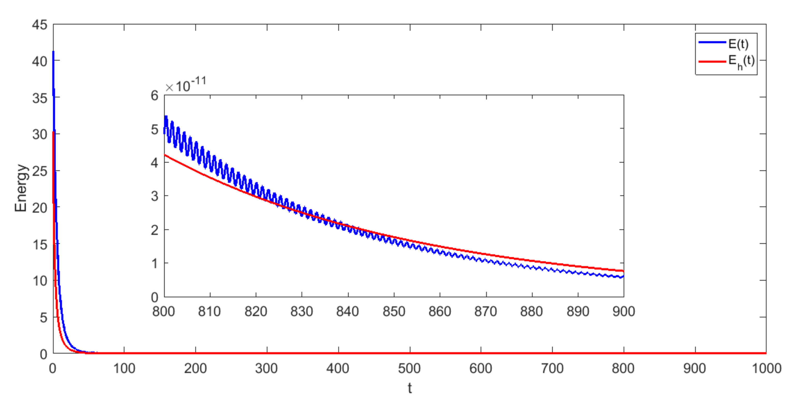
Consider the following relaxation function,
g ( t ) = a ( 1 + t ) ν , t 0 ,
for ν > 1 , and a is chosen so that hypothesis ( A ) remains valid. Then
g ( t ) = b H ( g ( t ) ) with ξ ( t ) = b and H ( s ) = s p ,
where b is a fixed constant, p = 1 + ν ν , which satisfies 1 < p < 2 . Thus, under the assumptions of Theorem 1, we conclude that the solution of (4) satisfies, for some constant C > 0 and t 1 > 0 , the energy estimate
E ( t ) C ( 1 + t ) ν , t > t 1 .

5. Numerical Tests

In this section, numerical experiments are performed to illustrate the energy decay results in Theorem 1. For this purpose, we developed a second-order numerical scheme to solve the problem (4) based on finite element discretization and the Crank–Nicolson method in time that has the property of being unconditionally stable.
The spatial interval ( 0 , L ) = ( 0 , 1 ) is subdivided into 100 sub-intervals, where the temporal interval ( 0 , T ) = ( 0 , 1000 ) is subdivided into N with a time step Δ t = T / N . We ran our code for N time steps ( N = T / Δ t ) using the following initial conditions:
z 0 ( x ) = sin ( π x ) , u 0 ( x ) = 2 sin ( π x ) ,
z 1 ( x ) = u 1 ( x ) = sin ( π 2 x )
The numerical tests are done in the light of the Example 1 as follows
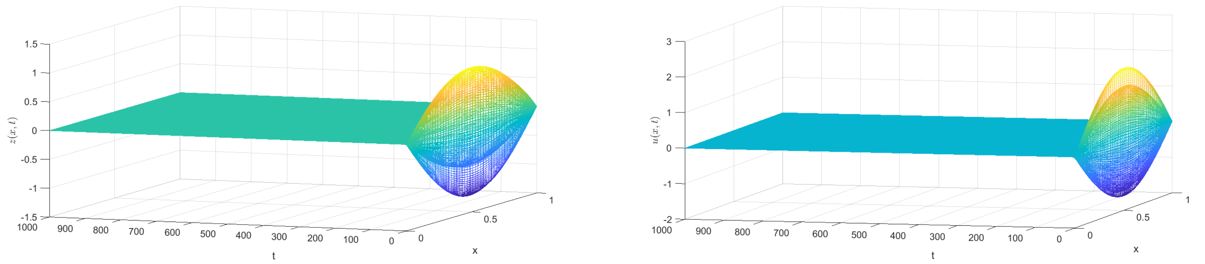
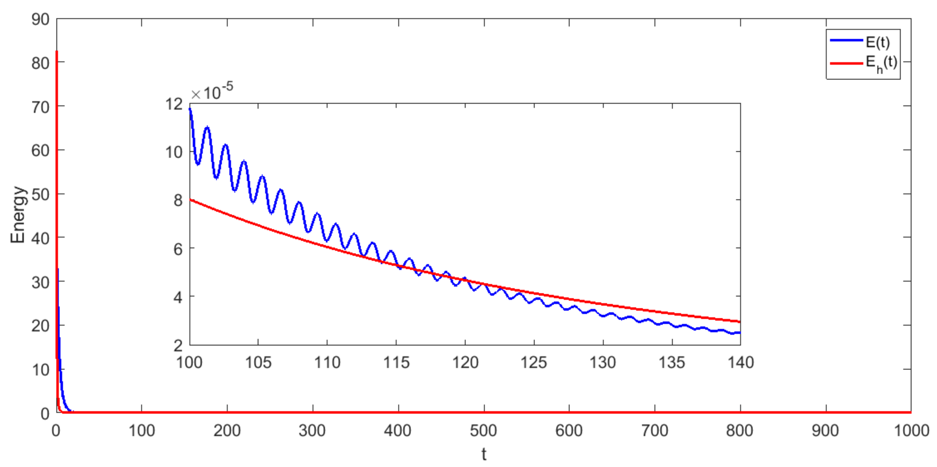
  • Test 1: For the first numerical test, we choose the following entries:
    ρ z = ρ u = a 1 = a 2 = 1 , a 3 = 2 ,
    and the relaxation function
    g ( t ) = e 2 t , t 0 .
    Thus, under the assumptions of Theorem 1, the solution of (4) satisfies the energy estimate
    E ( t ) E h ( t ) = C e 1 5 t , t > t 1
    where C is a constant depends on the energy at t = 0 .
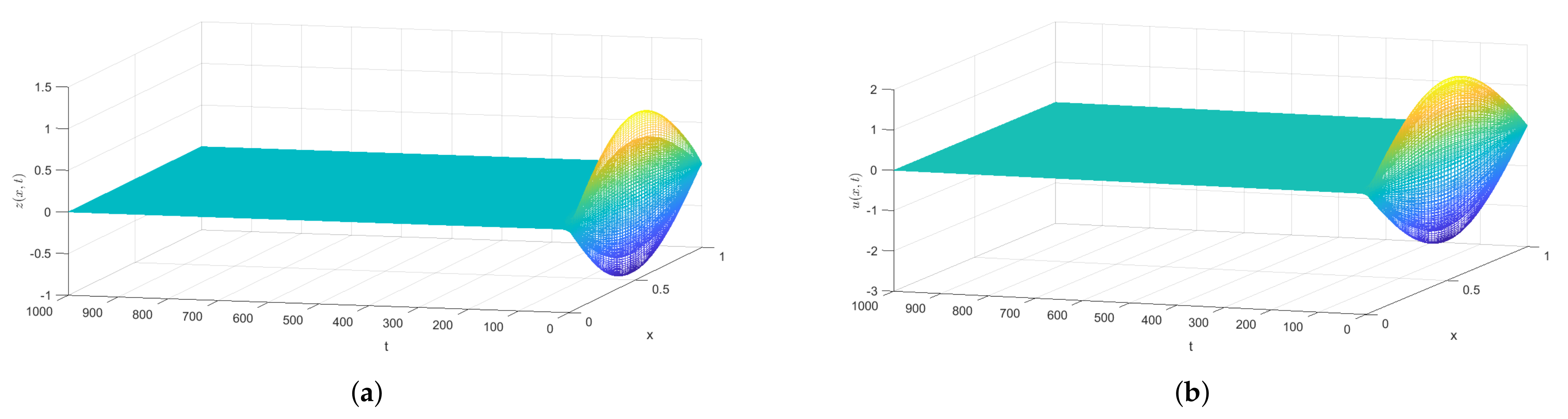
  • Test 2: In the second numerical test, we consider the following entries so that condition ( A ) is satisfied
    ρ z = ρ u = a 1 = a 2 = 1 , a 3 = 3
    and the following relaxation function
    g ( t ) = 1 3 e 1 + t , t 0
    Then, under the assumptions of Theorem 1, the solution of (4) satisfies the energy estimate
    E ( t ) E h ( t ) = C e 1 + t , for a t large enough
    where C is a constant depends on the energy at t = 0 .
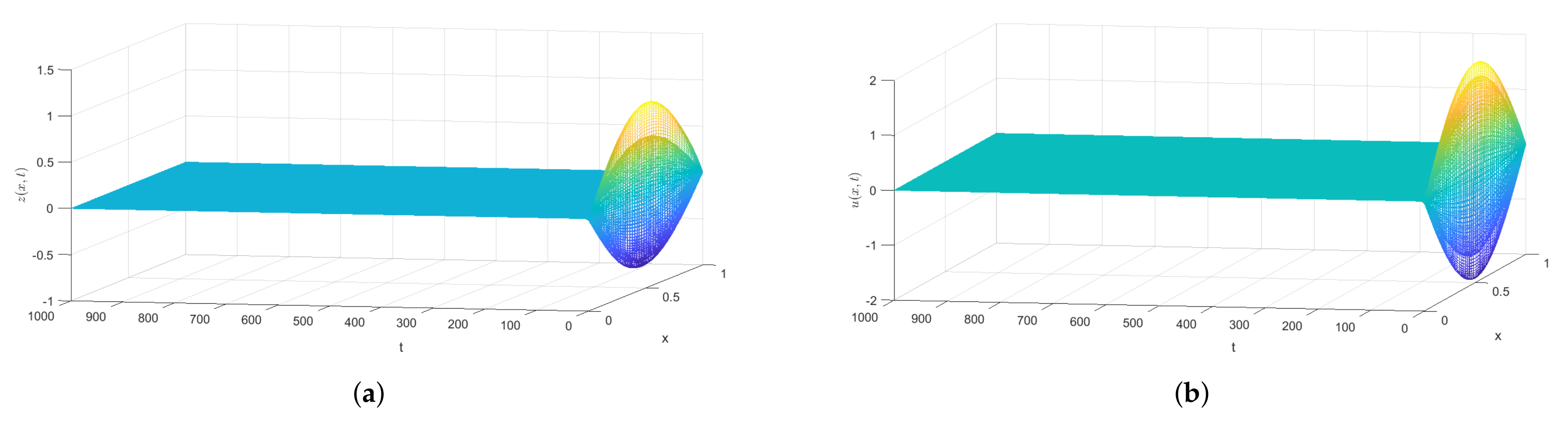
  • Test 3: For last test, we consider the third case of Example 1 with the same entries of Test 1 and with an polynomial relaxation function
    g ( t ) = 1 ( 1 + t ) 3 , t 0 .
    Under the assumptions of Theorem 1, the solution of (4) satisfies the energy estimate
    E ( t ) E h ( t ) = C 1 ( 1 + t ) 3 , t > t 1 ,
    where C is a constant depends on the energy at t = 0 .
For Test 1, we examine the exponential decay case. Under the initial and boundary conditions above, we plot in Figure 1 the decay behavior of the solution ( z , u ) in time and space. In Figure 2, we plot the energy decay and we made a zoom on the time interval [ 950 , 1000 ] to show the difference between the curves of E ( t ) and E h ( t ) and according to the parameters chosen in this test the time t 1 is too small.
Next, by following the same process, we present the numerical results of Test 2 in Figure 3 and Figure 4. We observed that the energy decay satisfies the energy inequality in Test 2, when the time is large enough that t 840 (as we can observe in the zoomed in part of Figure 4).
Finally, Figure 5 and Figure 6 show the results of Test 3, which are demonstrated the damping behavior. Furthermore, the energy inequality is satisfied for t 1 = 120 (as we can observe on the zoom part of Figure 6).
As a conclusion, we observed that the energy decay uniformly for all tests and satisfies the results of Theorem 1.

6. Conclusions

In this work, we considered a swelling porous elastic soil system with a viscoelastic damping term. We obtained a general decay result with a large class of the relaxation functions associated with the memory term. We also preformed numerical tests to justify our theoretical decay result. Our result generalizes the one of [18] and gives a sharper decay rate in specific cases.

Author Contributions

Conceptualization, A.M.A.-M. and M.M.A.-G.; methodology, A.M.A.-M. and M.M.A.-G.; software, M.A.; validation, A.M.A.-M. and M.M.A.-G.; formal analysis, A.M.A.-M. and M.M.A.-G.; investigation, A.M.A.-M. and M.M.A.-G.; resources, A.M.A.-M. and M.M.A.-G.; data curation, A.M.A.-M. and M.M.A.-G.; writing—original draft preparation, A.M.A.-M. and M.M.A.-G.; writing—review and editing, A.M.A.-M. and M.M.A.-G.; visualization, A.M.A.-M. and M.M.A.-G.; supervision, A.M.A.-M. and M.M.A.-G.; project administration, A.M.A.-M. and M.M.A.-G.; funding acquisition, A.M.A.-M. and M.M.A.-G. All authors have read and agreed to the published version of the manuscript.

Funding

This work is funded by KFUPM under ProjectSB201005.

Acknowledgments

The authors thank King Fahd University of Petroleum and Minerals (KFUPM) for the continuous support. The authors also thank the referees for their very careful reading and valuable comments. This work is funded by KFUPM under Project SB201005.

Conflicts of Interest

The authors declare that there is no conflict of interest.

References

  1. Coduto, D.P. Geotechnical Engineering: Principles and Practices; Prentice Hall: Hoboken, NJ, USA, 1999. [Google Scholar]
  2. Holtz, R.D.; Kovacs, W.D.; Sheahan, T.C. An Introduction to Geotechnical Engineering; Prentice-Hall: Englewood Cliffs, NJ, USA, 1981; Volume 733. [Google Scholar]
  3. Kalantari, B. Construction of Foundations on Expansive Soils; University of Missouri Columbia: Columbia, MI, USA, 1991. [Google Scholar]
  4. Hung, V. Hidden Disaster. In University News; University of Saska Techwan: Saskatoon, SK, Canada, 2003. [Google Scholar]
  5. Freitas, M.M.; Ramos, A.J.; Santos, M.L. Existence and Upper-Semicontinuity of Global Attractors for Binary Mixtures Solids with Fractional Damping. Appl. Math. Optim. 2019, 83, 1353–1385. [Google Scholar] [CrossRef]
  6. Karalis, T. On the elastic deformation of non-saturated swelling soils. Acta Mech. 1990, 84, 19–45. [Google Scholar] [CrossRef]
  7. Handy, R.L. A stress path model for collapsible loess. In Genesis and Properties of Collapsible Soils; Springer: Berlin/Heidelberg, Germany, 1995; pp. 33–47. [Google Scholar]
  8. Leonard, R. Expansive Soils Shallow Foundation; Regent Centre, University of Kansas: Lawrence, KS, USA, 1989. [Google Scholar]
  9. Jones, L.D.; Jefferson, I. Expansive Soils. In ICE Manual of Geotechnical Engineering Vol 1: Geotechnical Engineering Principles, Problematic Soils and Site Investigation (ICE Manuals); ICE Publishing: London, UK, 2012; pp. 413–441. [Google Scholar]
  10. Bowles, J.E. Foundation Design and Analysis; McGraw-Hill: New York, NY, USA, 1982. [Google Scholar]
  11. Kalantari, B. Engineering significant of swelling soils. Res. J. Appl. Sci. Eng. Technol. 2012, 4, 2874–2878. [Google Scholar]
  12. Krauklis, A.E.; Gagani, A.I.; Echtermeyer, A.T. Prediction of orthotropic hygroscopic swelling of fiber-reinforced composites from isotropic swelling of matrix polymer. J. Compos. Sci. 2019, 3, 10. [Google Scholar] [CrossRef] [Green Version]
  13. Sinchuk, Y.; Pannier, Y.; Gueguen, M.; Tandiang, D.; Gigliotti, M. Computed-tomography based modeling and simulation of moisture diffusion and induced swelling in textile composite materials. Int. J. Solids Struct. 2018, 154, 88–96. [Google Scholar] [CrossRef]
  14. Ieşan, D. On the theory of mixtures of thermoelastic solids. J. Therm. Stress. 1991, 14, 389–408. [Google Scholar] [CrossRef]
  15. Quintanilla, R. Exponential stability for one-dimensional problem of swelling porous elastic soils with fluid saturation. J. Comput. Appl. Math. 2002, 145, 525–533. [Google Scholar] [CrossRef] [Green Version]
  16. Wang, J.M.; Guo, B.Z. On the stability of swelling porous elastic soils with fluid saturation by one internal damping. IMA J. Appl. Math. 2006, 71, 565–582. [Google Scholar] [CrossRef]
  17. Ramos, A.; Freitas, M.; Almeida, D., Jr.; Noé, A.; Santos, M.D. Stability results for elastic porous media swelling with nonlinear damping. J. Math. Phys. 2020, 61, 101505. [Google Scholar] [CrossRef]
  18. Apalara, T.A. General stability result of swelling porous elastic soils with a viscoelastic damping. Z. Angew. Math. Phys. 2020, 71, 200. [Google Scholar] [CrossRef]
  19. Pamplona, P.X.; Rivera, J.E.M.; Quintanilla, R. Stabilization in elastic solids with voids. J. Math. Anal. Appl. 2009, 350, 37–49. [Google Scholar] [CrossRef] [Green Version]
  20. Magaña, A.; Quintanilla, R. On the time decay of solutions in porous-elasticity with quasi-static microvoids. J. Math. Anal. Appl. 2007, 331, 617–630. [Google Scholar] [CrossRef] [Green Version]
  21. Muñoz-Rivera, J.; Quintanilla, R. On the time polynomial decay in elastic solids with voids. J. Math. Anal. Appl. 2008, 338, 1296–1309. [Google Scholar] [CrossRef] [Green Version]
  22. Soufyane, A. Energy decay for porous-thermo-elasticity systems of memory type. Appl. Anal. 2008, 87, 451–464. [Google Scholar] [CrossRef]
  23. Messaoudi, S.A.; Fareh, A. General decay for a porous-thermoelastic system with memory: The case of nonequal speeds. Acta Math. Sci. 2013, 33, 23–40. [Google Scholar] [CrossRef]
  24. Apalara, T.A. General decay of solutions in one-dimensional porous-elastic system with memory. J. Math. Anal. Appl. 2019, 469, 457–471. [Google Scholar] [CrossRef]
  25. Apalara, T.A. A general decay for a weakly nonlinearly damped porous system. J. Dyn. Control Syst. 2019, 25, 311–322. [Google Scholar] [CrossRef]
  26. Feng, B.; Apalara, T.A. Optimal decay for a porous elasticity system with memory. J. Math. Anal. Appl. 2019, 470, 1108–1128. [Google Scholar] [CrossRef]
  27. Feng, B.; Yin, M. Decay of solutions for a one-dimensional porous elasticity system with memory: The case of non-equal wave speeds. Math. Mech. Solids 2019, 24, 2361–2373. [Google Scholar] [CrossRef]
  28. Casas, P.S.; Quintanilla, R. Exponential decay in one-dimensional porous-thermo-elasticity. Mech. Res. Commun. 2005, 32, 652–658. [Google Scholar] [CrossRef] [Green Version]
  29. Santos, M.; Campelo, A.D.S.; Almeida Júnior, D.A. On the decay rates of porous elastic systems. J. Elast. 2017, 127, 79–101. [Google Scholar] [CrossRef]
  30. Apalara, T.A. General stability of memory-type thermoelastic Timoshenko beam acting on shear force. Contin. Mech. Thermodyn. 2018, 30, 291–300. [Google Scholar] [CrossRef]
  31. Ammar-Khodja, F.; Benabdallah, A.; Rivera, J.M.; Racke, R. Energy decay for Timoshenko systems of memory type. J. Differ. Equ. 2003, 194, 82–115. [Google Scholar] [CrossRef] [Green Version]
  32. Al-Mahdi, A.M.; Al-Gharabli, M.M.; Guesmia, A.; Messaoudi, S.A. New decay results for a viscoelastic-type Timoshenko system with infinite memory. Z. Angew. Math. Phys. 2021, 72, 22. [Google Scholar] [CrossRef]
  33. Al-Mahdi, A.M.; Al-Gharabli, M.M.; Alahyane, M. Theoretical and numerical stability results for a viscoelastic swelling porous-elastic system with past history. AIMS Math. 2021, 6, 11921–11949. [Google Scholar] [CrossRef]
  34. Alabau-Boussouira, F.; Cannarsa, P. A general method for proving sharp energy decay rates for memory-dissipative evolution equations. Comptes Rendus Math. 2009, 347, 867–872. [Google Scholar] [CrossRef] [Green Version]
  35. Mustafa, M.I. Optimal decay rates for the viscoelastic wave equation. Math. Methods Appl. Sci. 2018, 41, 192–204. [Google Scholar] [CrossRef]
  36. Jin, K.P.; Liang, J.; Xiao, T.J. Coupled second order evolution equations with fading memory: Optimal energy decay rate. J. Differ. Equ. 2014, 257, 1501–1528. [Google Scholar] [CrossRef]
  37. Arnold, V. Mathematical Methods of Classical Mechanics; Springer: Berlin, Germany; New York, NY, USA, 1989. [Google Scholar]
Figure 1. Test 1: The approximate solution ( z , u ) in the x-t plane. (a) z ( x , t ) . (b) u ( x , t ) .
Mca 27 00027 g001
Figure 2. Test 1: energy decay.
Mca 27 00027 g002
Figure 3. Test 2: The approximate solution ( z , u ) in the x-t plane. (a) z ( x , t ) . (b) u ( x , t ) .
Mca 27 00027 g003
Figure 4. Test 2: energy decay.
Mca 27 00027 g004
Figure 5. Test 3: The approximate solution ( z , u ) in the x-t plane. (a) z ( x , t ) . (b) u ( x , t ) .
Mca 27 00027 g005
Figure 6. Test 3: energy decay.
Mca 27 00027 g006
Publisher’s Note: MDPI stays neutral with regard to jurisdictional claims in published maps and institutional affiliations.

