Interval-Based Computation of the Uncertainty in the Mechanical Properties and the Failure Analysis of Unidirectional Composite Materials

Abstract

An interval-based method is presented to evaluate the uncertainty in the computed mechanical properties and the failure assessment of composite unidirectional (UD) laminates. The method was applied to two composite laminates: a carbon/epoxy and a glass/epoxy. The mechanical properties of the UD lamina were derived using simplified micromechanical equations. An uncertainty level of ±5% was assumed for the input properties of the constituents. The global minimum and maximum values of the properties were computed using an interval branch-and-bound algorithm. Interval arithmetic operations were used to evaluate the uncertainty in the Hashin-type failure criteria in a closed form. Using the closed-form uncertainties of intervals and sets of stresses obtained by finite element analysis, the uncertainty in the failure assessment was quantified for the two composite laminates. For the assumed uncertainty level of ±5%, the computed uncertainty for the mechanical properties ranges from 6.64% to 10.63% for the carbon/epoxy material and from 6.72% to 12.28% for the glass/epoxy material. For evaluating the uncertainty effect on the efficiency of failure criteria, a probability of failure function, which employs interval boundaries, was defined and proved capable of evaluating the whole spectrum of stresses.

1. Introduction

Fiber-reinforced composites, especially carbon-fiber-reinforced plastics (CFRPs), have become the primary structural material of lightweight structures [1]. At the same time, the numerical design of composite structures finds an increasing use in aiming to reduce the time and cost of the development and design phases.

Micromechanics of composites is the branch of mechanics of composites that predicts the elastic properties and strengths of a unidirectional lamina by using the properties of the fibers and the matrix. Due to the anisotropy and inhomogeneity of composites, the complete experimental characterization of their mechanical properties requires many tests that must be conducted by using different lay ups and loading conditions. There have been proposed several sets of micromechanical analytical relations in the literature. The most widely used set is the one proposed by Chamis [2]. For the failure analysis of UD composites, the several sets of failure criteria are mainly due to the diversity of composite materials [3]. Each set is suitable for a specific type of composite materials and specific loading conditions. A widely used set is the Hashin-type failure criteria [4]. They are of a polynomial type, are stress based, and can distinguish between the different failure modes. Moreover, they have high accuracy and are highly compatible with the finite element (FE) method. Due to the above characteristics, they have been extensively used in progressive-damage models [5,6,7,8].

The computational efficiency of micromechanical equations and the failure criteria depends on the experimental error. The scatter of the results is higher for composites than for monolithic materials due to the material’s complexity, the involvement of different types of tests, and the presence of manufacturing defects. It is, therefore, of great importance to quantify the uncertainty of the predictions of micromechanical equations because it reflects the computation of stresses and strains and the predicted damage, thus compromising the performance of composite components, leading to the use of more conservative designs that do not fully exploit the performance and environmental opportunities offered by composites. Mainly, manufacturing uncertainties can be summarized as follows: (a) fibre architecture variations that are usually generated during production, handling, or storage of prepregs, dry textiles, and per-forms, (b) matrix material uncertainties caused by variations in storage conditions or uncertainties in resin composition and formulation, and (c) variations in environmental parameters and process conditions.

The majority of the works reported in the literature for quantifying uncertainty in the mechanical properties of UD composites are based on probabilistic approaches [9]. In addition, Monte-Carlo methods have also been used based on assumed probability distributions [10]. However, Monte-Carlo methods are computationally demanding and unsuitable for complex material systems and parts of a larger scale. On the other hand, interval analysis has been used in multidisciplinary engineering applications such as in the formulation of fuzzy finite elements [11], the time-dependent reliability analysis of fatigue crack growth [12], and structural optimization [13].

In recent works, Alazwari and Rao [14,15] performed uncertainty quantification of the micromechanical properties of composite materials. Moreover, in [16], two different versions of the interval-based uncertainty failure model, based on the maximum stress failure theory and the Tsai–Wu failure theory, using the universal gray system theory and the truncation-based interval analysis, were presented. These are the only published works on the interval approach to quantify uncertainty in the micromechanical properties of UD composites; however, they do not include the quantification of uncertainty in the failure analysis.

Although there are numerous numerical methods for approximating the range of real functions, none of them guarantee the required accuracy of the result, and the majority of them (e.g., Monte Carlo) face computational-time constraints. However, the main advantage of interval arithmetic is inclusion isotonicity, a valuable property in connection with the fundamental theorem [17,18] of interval analysis that guarantees the production of reliable numerical solutions with mathematical correctness. Since the uncertainty problem is equivalent to bounding the range of a multivariate function over a multidimensional rectangle (box), interval mathematics is the most straightforward technique for modeling uncertainty and providing guaranteed enclosures. When the interval parameters of a multivariate function are large, it can be challenging to determine its exact range. This paper proposes an efficient interval algorithm with mathematical correctness to solve this problem.

The article is organized into five sections. In Section 2, we briefly introduce the basics of interval arithmetic, the mean value form, and the corresponding optimal center. In Section 3, we present our computational method based on a rigorous interval branch-and-bound algorithm for computing the range of a multivariate function with large-range uncertain parameters. Section 4 presents the computed uncertainties in the elastic properties and strengths of two UD composite laminae and the sensitivity analysis of the elastic properties. Section 5 describes the methodology and results of the uncertainty in the failure assessment of the composite laminae, performed using the Hashin-type failure criteria. The paper is completed with three Appendices in which we exhibit the Chamis micromechanical equations, the Hashin-type failure criteria, and equations for the computation of uncertainty intervals of the criteria.

2. Interval Analysis

This section presents the interval mathematics required for the rest of the paper. We provide only a summary of basic interval definitions and properties; for a more in-depth discussion, see, for example, [17,18,19]. Interval arithmetic [17] generalizes ordinary arithmetic to closed intervals of the real line. Let $I(ℝ)=\left\{[a,b]\hspace{0.17em}|\hspace{0.17em}a\le b,\hspace{0.17em}a,b\in ℝ\right\}$ be the set of real closed intervals and $I({ℝ}^n)$ the $n$-dimensional interval vectors (also called boxes). Given a pair of intervals $X=[\underset{\_}{x},\overline{x}]$ and $Y=[\underset{\_}{y},\overline{y}]$ with $0\notin Y$, the four basic interval arithmetic operations are defined by

$$\begin{array}{l}X+Y=[\underset{\_}{x}+\underset{\_}{y},\hspace{0.17em}\overline{x}+\overline{y}],\\ X-Y=[\underset{\_}{x}-\overline{y},\hspace{0.17em}\overline{x}-\underset{\_}{y}],\\ X\times Y=[\min (\underset{\_}{x}\hspace{0.17em}\underset{\_}{y},\hspace{0.17em}\underset{\_}{x}\hspace{0.17em}\overline{y},\overline{x}\hspace{0.17em}\underset{\_}{y},\overline{x}\hspace{0.17em}\overline{y}),\hspace{0.17em}\max (\underset{\_}{x}\hspace{0.17em}\underset{\_}{y},\hspace{0.17em}\underset{\_}{x}\hspace{0.17em}\overline{y},\overline{x}\hspace{0.17em}\underset{\_}{y},\overline{x}\hspace{0.17em}\overline{y})],\\ X/Y=X\cdot [1/\overline{y},1/\underset{\_}{y}],\hspace{0.17em}\hspace{0.17em}\mathrm{if}\hspace{0.17em}\hspace{0.17em}0\notin Y.\end{array}$$

It is worth noting that the above elementary operations are inclusion isotonic, which means: if $X\subseteq Y$ and $X^{\prime }\subseteq Y^{\prime }$ then $X\circ Y\subseteq X^{\prime }\circ Y^{\prime }$ for each binary operation $\circ \in \left\{+,-,\times ,/\right\}$. In practice, rounded interval arithmetic is utilized to bound roundoff error instead of the exact form above. Rounded intervals may be somewhat larger, but they always contain the exact result [20]. The same interval $X\in I(ℝ)$ can be defined in three ways: either by its endpoints, or by its midpoint $m(X)=(\underset{\_}{x}+\hspace{0.17em}\overline{x})/2$ and radius $r(X)=\hspace{0.17em}(\overline{x}-\underset{\_}{x})/2$ as $X=\left[m\left(X\right)-r\left(X\right),m\left(X\right)+r\left(X\right)\right]$, and, lastly, in terms of its midpoint and its uncertainty level $\lambda$ as $X=m\left(X\right)[1-\lambda ,1+\lambda ]$, where $\lambda =r(X)/|m(X)|$. Sometimes, for clarity, the lower bound of $X$ is also denoted as $\inf X$, and the upper bound is denoted $\sup X$.

Let $f_{rg}(X)$ denote the range of the function $f:{ℝ}^n\to ℝ$ over an interval vector $X\in I({ℝ}^n)$, i.e., $f_{rg}(X)=\left\{\underset{x\in X}{\min }f(x),\hspace{0.17em}\underset{x\in X}{\max }f(x)\right\}$. A function $F:I({ℝ}^n)\to I(ℝ)$ is called an inclusion function of $f$ if $f_{rg}(X)\subseteq F(X)$ for any $X\in I({ℝ}^n)$. It is well-known that any intersection of inclusion functions is an inclusion function. Natural extension, mean value forms, and Taylor expansion create inclusion functions [17] that are inclusion isotones, i.e., $\forall X,Y\in I({ℝ}^n),\hspace{0.17em}X\subseteq Y\Rightarrow F(X)\subseteq F(Y)$. Each of these forms has slightly different properties and convergence orders. For a thorough discussion on these issues, see [19].

Optimal Mean Value Form

Assuming that $f$ is continuously differentiable, the gradient’s inclusion function $\nabla f$ may be computed (for almost any function specified by a finite procedure) employing automatic differentiation [21] and interval arithmetic. The most important centered form is the mean value form (MVF), which is obtained by taking the first order of Taylor’s expression:

$$F_{MVF}\left(X,c\right)=f\left(c\right)+{\left(X-c\right)}^T\nabla F\left(X\right)=f(c)+{\displaystyle \sum _{i=1}^n{G}_i\left(X\right)\left(X_i-c_i\right)}$$

(1)

where $X$ is an $n$-dimensional vector of intervals $X_i=[{\underset{\_}{x}}_i,{\overline{x}}_i]$, $i=1,\dots ,n$ $c=m(X)=\left(c_1,\dots ,c_n\right)$ is the midpoint of the box $X$, and $G_i\left(X\right)=[{\underset{\_}{g}}_i,{\overline{g}}_i]$ is the interval extension of the derivative $\partial f/\partial x_i$. A second-order approximation to the range of $f$ is proved in [22,23] and the isotonicity property when the center $c$ is the midpoint. The mean value form $F_{MVF}$ ensures tighter enclosures than the natural interval extension $F$ when the interval $X$ is narrow. Nevertheless, on the other hand, when the diameter of $X$ is large, $F_{MVF}$ may drastically overestimate the range of $f$. Consequently, it is common to use the intersection $F_{MVF}\left(X,c\right)\cap F(X)$ to obtain a more accurate range estimate.

In [24], Baumann introduced the notion of optimal mean value forms and proved a weaker property called one-sided isotonicity for the produced forms, a valuable property that in the framework of global minimization algorithms suffices. The point $c^{-}$, which yields the greatest lower bound, and the point $c^{+}$, which yields the lowest upper bound among all centers $c\in X$, are called optimal centers. Baumann provided asymmetric formulas for these centers; while, in [25], the authors determined in a straightforward manner equivalent symmetric expressions for the optimal centers, and they proved the conjecture that the width of (1) is minimal for all centers between $c^{-}$ and $c^{+}$. Furthermore, exact formulas for the lower and upper bounds of optimal MVFs are provided, which show that there is no need for the box’s width to tend to zero to have sharp bounds. The lower bound of the MVF attains its maximum at the center $c^{-}={\left(c_1^{-},\dots ,c_n^{-}\right)}^T\in {ℝ}^n$ with components [25]:

$$c_i^{-}=\left\{\begin{array}{ccc}{\overline{x}}_i,& if& {\overline{g}}_i\le 0,\\ {\underset{\_}{x}}_i,& if& {\underset{\_}{g}}_i\ge 0,\\ m(X_i)-r(X_i)\hspace{0.17em}\frac{{\overline{g}}_i+{\underset{\_}{g}}_i}{{\overline{g}}_i-{\underset{\_}{g}}_i},& & otherwise.\end{array}\right.$$

(2)

In order to determine the optimal center $c^{+}$ for the best upper bound of MVF, the optimal point $c^{-}$ should be mirrored about the midpoint $m(X)$, resulting in $c^{+}=m(X)+[m(X)-c^{-}]$, since the optimal centers $c^{-}$ and $c^{+}$ are always symmetric concerning the midpoint (see [25]).

For simplicity of notation, the left endpoint of the interval $F_{MVF}(X,c^{-})$ will be denoted by $\inf F_{MVF}(X,c^{-})$. Let $I_0$ be the subset of the index set $I=\{1,\dots ,n\}$, where $i\in I_0$ if $0\in G_i(X)=[{\underset{\_}{g}}_i,{\overline{g}}_i]$, then it can be proved [26] that the lower bound of the MVF (1) with center $c^{-}$ is given by:

$$\inf F_{MVF}(X,c^{-})=f(c^{-})+{\displaystyle \sum _{i\in I_0}w(X_i)\hspace{0.17em}\frac{{\overline{g}}_i\cdot {\underset{\_}{g}}_i}{{\overline{g}}_i-{\underset{\_}{g}}_i}}$$

(3)

where $w(X_i)={\overline{x}}_i-{\underset{\_}{x}}_i$ denotes the width of the interval $X_i$ [25]. It is evident that when the function $f$ is strictly monotone over an interval vector $X$, then $I_0=\varnothing$ and, therefore, $\inf F_{MVF}(X,c^{-})$ is the exact lower bound; in a different case, $\inf F_{MVF}(X,c^{-})$ is overestimated, and we must determine a coordinate direction to bisect the box $X$.

The adopted selection rule for subdividing the box is inspired by Equation (3), and our goal is to maximize the lower bound of the inclusion function after each subdivision. We observe that, for all $i\in I_0$, the summation terms are all negative; therefore, to maximize the lower bound of MVF, the optimal component $k\in I_0$ is determined by the largest absolute summation term, which subtracts the most. This selection rule is very similar to Ratz’s rule C [26,27], where the goal was to minimize the width of the inclusion in Equation (2).

Our algorithm, presented in Section 3, uses first-order information through an interval gradient evaluation and takes advantage of the valuable properties of the optimal center (2) of the MVF for both the bounding and the branching process.

3. The Proposed Branch-and-Bound Algorithm

This section introduces an interval branch-and-bound algorithm for computing the range

$$F^{\ast }=\left[\underset{x\in X}{\min }f(x),\hspace{0.17em}\underset{x\in X}{\max }f(x)\right]$$

(4)

of a continuously differentiable function $f:{ℝ}^n\to ℝ$ over a box $X$ to solve uncertainty problems with large-range interval parameters. As the maximization problem can be transformed into a minimization problem, precisely, $\max f(x)\equiv -\left[\min (-f(x))\right]$, the proposed algorithm aims to compute verified enclosures for the global minimum of functions.

Algorithm 1 formulates the main procedure in pseudo-code. In Step 1, we first find a guaranteed lower bound, $F_{\min }^{\ast }$, on the range of values of $f$ over the search box $X^0$, and then apply the same procedure in Step 2, to find a lower bound on $(-f)$ over $X^0$ to obtain the upper bound, $F_{\max }^{\ast }$. Finally, in Step 3, we determine the enclosure $F^{\ast }$ of the range from the previous two steps.

Algorithm 1. ComputeRange $\left(f,X^0,\epsilon ,F^{\ast }\right)$

Input: objective function $f$, starting box $X^0$, and tolerance $\epsilon$ Output: enclosure $F^{\ast }$ of the range 1: $\mathrm{GlobalMinimize}\left(f,X^0,\epsilon ,F_{\min }^{\ast }\right)$; 2: $\mathrm{GlobalMinimize}\left(-f,X^0,\epsilon ,F_{\max }^{\ast }\right)$; 3: $F^{\ast }=\left[\inf F_{\min }^{\ast },\hspace{0.17em}\sup \left(-F_{\max }^{\ast }\right)\right]$; 4: return $F^{\ast }$;

Algorithm 2 describes the branch-and-bound interval algorithm we implemented, employing two well-known accelerating devices: the cut-off test and the monotonicity test [21,26]. The algorithm uses first-order information of the objective function utilizing an interval gradient evaluation, firstly, to check monotonicity and then apply the optimal mean value form for bounding the range of the function. For bounding the objective function, we take the intersection of the natural interval extension $F(X)$ with optimal mean value form $F_{MVF}(X,c^{-})$ to obtain the best lower bound for the range of $f$. Moreover, as discussed in the previous, Section Optimal Mean Value Form, the calculated derivative bounds are exploited to determine an optimal component $k$ (subdivision direction) to bisect the box during the branching phase of the algorithm.

In general, the search tree is incrementally expanded by iterating the following steps: (i) the initial search box $X^0$ is subdivided into smaller sub-boxes, (ii) the objective function and its derivatives are bounded over the sub-boxes, and (iii) sub-boxes that cannot contain a global minimizer with certainty are removed. We next summarize the basic interval techniques that accelerate the search process:

• Function range test: A box $Y$ is discarded from further consideration when the lower bound $\inf F_Y$ is greater than the current upper bound $f_{\max }$. When the range test fails to remove it, it is stored in the working list with candidate sub-boxes for further investigation.
• Cut-off test: The function range test is applied for all candidate sub-boxes in the working list when $f_{\max }$ is improved. Of course, the greater the improvement in $f_{\max }$ is, the more influential the cut-off test is.
• Monotonicity test: Determines whether the objective function $f$ is strictly monotone in an entire sub-box $Y\subset X^0$ or at least one coordinate direction, in which case $Y$ cannot contain a global minimizer. Therefore, the whole sub-box is discard or its dimension reduced as much as possible when $Y\subseteq X^0$.

We now give a detailed algorithmic description of our proposed method (Algorithm 2), implemented in C++ using the C-XSC-2.5 library (http://www.math.uni-wuppertal.de/~xsc/ (accessed on 25 March 2022).

Algorithm 2. GlobalMinimize $\left(f,X^0,\epsilon ,F^{\ast }\right)$

Input: objective function $f$, starting box $X^0$, and tolerance $\epsilon$ Output: enclosure $F^{\ast }$ for the global minimum value 01: $Y=X^0$; $L=\{\hspace{0.17em}\};$ $L^{\ast }=\{\hspace{0.17em}\};$                /* initialize working and result list */ 02: $\mathrm{MonotonicityTest}\left(X^0,Y,\nabla F\left(Y\right)\hspace{0.17em},del\right);$            /* apply monotonicity test */ 03: $c=\mathrm{OptimalCenter}\left(Y,\nabla F(Y)\right)$;        /* compute optimal center using Equation (2) */ 04: $f_{\max }=\sup F(c)$;                /* initialize upper bound for global minimum */ 05: $F_Y=\left(F(c)+\nabla F(Y)(Y-c)\right)\cap F(Y)$;             /* optimal mean value form */ 06: $k=\mathrm{OptimalComp}\left(Y,\nabla F(Y)\right)$;        /* optimal component for subdividing the box */ 07: if $k=0$ then $L^{\ast }=L^{\ast }\cup \left(Y,\inf F_Y,k\right)$;   /* no subdivision required, append to the result list */ 08: else $L=L\cup \left(Y,\inf F_Y,k\right)$;                    /* append to working list */ 09: while $L\ne \{\hspace{0.17em}\}$ do 10:  $\left(Y,\inf F_Y,k\right)=\mathrm{PopHead}\left(L\right)$;         /* remove a triple from the head of the working list */ 11:  if $k\ne 0$ then Bisect $\left(Y,k,U_1,U_2\right)$;             /* subdivide $Y$ into two subboxes */ 12:  for $i=1$ to NBoxes do                    /* number of boxes is 1 if $k=0$ */ 13: if $\inf F\left(U_i\right)\hspace{0.17em}>f_{\max }$ then next $i$;       /* box $U_i$ is discarded due to function range test */ 14: $\mathrm{MonotonicityTest}\left(X^0,U_i,\nabla F\left(U_i\right)\hspace{0.17em},del\right);$ 15: if $del==true$ then next $i$;          /* box $U_i$ is discarded due to monotonicity test */ 16: $c=\mathrm{OptimalCenter}\left(U_i,\nabla F\left(U_i\right)\right)$;      /* compute optimal center using Equation (2) */ 17: if $\sup F(c)<f_{\max }$ then                /* update upper bound $f_{\max }$ if possible */ 18:  $f_{\max }=\sup F(c)$; $\mathrm{CutOffTest}\left(L,\hspace{0.17em}{f}_{\max }\right)$;            /* and apply cut-off test */ 19: $F_U=\left(F(c)+\nabla F\left(U_i\right)(U_i-c)\right)\cap F(U_i)$;      /* optimal mean value form for box $U_i$*/ 20: if $\inf \hspace{0.17em}{F}_U>f_{\max }$ then next $i$;          /* box $U_i$ is discarded due to function range test */ 21: $k=\mathrm{OptimalComp}\left(U_i,\nabla F\left(U_i\right)\right);$          /* optimal component for subdividing $U_i$*/ 22: if $w_{rel}\left([\inf \hspace{0.17em}{F}_U,f_{\max }]\right)\le \epsilon$ or $\left(k=0\right)$ then $L^{\ast }=L^{\ast }\cup \left(U_i,\inf F_U,k\right)$; 23: else $L=L\cup \left(U_i,\inf F_U,k\right)$; 24: $\left(Y,\inf F_Y,k\right)=\mathrm{Head}\left(L^{\ast }\right)$;            /* set $Y$ to the first element of the result list */ 25: $F^{\ast }=\left[\inf F_Y,\hspace{0.17em}{f}_{\max }\right]$;               /* construct the global minimum enclosure. */ 26: return $F^{\ast }$;

Initially, the working list $L$ and the result list $L^{\ast }$ are empty. Following the evaluation of $\nabla F(Y)$, the monotonicity test is called to possibly reduce the dimension of the original box, and then compute the optimal center $c^{-}$ using Equation (2). The upper bound $f_{\max }$ is initialized by evaluating $F(c^{-})$ using interval arithmetic to bound all rounding errors. In Step 5, we bound the range of $f$ over $Y$ using the intersection $F_{MVF}\left(Y,c^{-}\right)\cap F(Y)$. While, in Step 6, the optimal component $k$ is determined by finding the largest absolute summation term of the expression in Equation (4). The value $k=0$ indicates that $f$ is strictly monotone over the entire box $Y$ or, in other words, the subset $I_0=\varnothing$. Then $\inf F_{MVF}(Y,c^{-})$ is the exact lower bound, and, therefore, no subdivision is required and the box is stored in the result list $L^{\ast }$. In Step 8, the box is stored in the working list $L$, in a different case. It is essential to notice that, when $k=0$, the total cost of the algorithm is two function evaluations and one gradient evaluation, the working list remains empty, and the algorithm jumps to Step 24.

The search is carried out by prioritizing the sub-boxes $Y$ using the best-first strategy [21,26]. The rationale for this strategy is to concentrate on the most promising box; that is, the one with the lowest lower bound because we are looking for the global minimum. This task can be accomplished quickly by using and maintaining a priority queue or list sorted in a non-decreasing order relative to the lower bounds $\inf F_Y$.

Steps 10–23 are applied to each candidate sub-box $Y$ until the working list $L$ is empty. The algorithm removes the first element from $L$ and subdivides the box $Y$ in the coordinate direction $k$. Special care is taken to handle unnecessary subdivisions if it has previously been proved that $f$ is strictly monotone. For each sub-box (one or two), first, the function range test (Step 13) is applied, and then the monotonicity test algorithm as proposed by Ratz [26]. When the upper bound $f_{\max }$ is improved, Steps 17–18, the cut-off test is applied to the working list $L$ to discard sub-boxes that definitely do not contain the global minimum. After bounding the range of $f$ over $U_i$, the range test is performed in Step 20 and $U_i$ is either added to the result list $L^{\ast }$ or the working list $L$, depending on the termination criterion (Steps 22–23). A box is stored in the result list when the relative diameter [21] of $F^{\ast }$ is smaller than a prescribed accuracy $\epsilon$ (defined by the user). When no candidate sub-boxes are contained in the working list, the algorithm terminates by returning an enclosure for the global minimum $F^{\ast }$.

Several examples have been investigated to test the algorithm’s correctness and efficiency. The inclusion functions have been implemented using the C-XSC routines while the gradients are computed with forward automatic differentiation [22]. All computations, including those involving floating-point numbers, were carried out using rounded interval arithmetic. Although we present the results with fewer digits, the bounds of the range were calculated with 14 significant digits accuracy. Therefore, we have set $\epsilon =(1/2)\times {10}^{-14}$.

To summarize, Algorithm 2 makes three uses of first-order information. Firstly, the monotonicity test can eliminate or reduce the current sub-box. Second, determining optimal MVF centers while simultaneously attempting to improve the global minimum’s current upper bound. Thirdly, using optimal MVF to improve the function range’s enclosure and use a more sophisticated subdivision rule when necessary.

4. Uncertainty Computation in the Elastic Properties and Strengths

The algorithm of Section 3 was applied for the uncertainty computation of the elastic properties and strengths of two different composite plies that find extensive use in the aeronautical and automotive industries, namely, the carbon/epoxy AS4/3501-6 composite ply and the glass/epoxy 21xK43-LY556 composite ply.

The elastic properties of the UD lamina considered are:

• E₁₁ = longitudinal Young’s modulus (fibers direction);
• E₂₂ = transverse Young’s modulus (normal to fibers);
• E₃₃ = normal Young’s modulus (normal to lamina);
• G₁₂ = in-plane shear modulus;
• G₁₃ = out-of-plane shear modulus;
• G₂₃ = out-of-plane shear modulus;
• ν₁₂ = in-plane Poisson’s ratio;
• ν₁₃ = out-of-plane Poisson’s ratio;
• ν₂₃ = out-of-plane Poisson’s ratio.

The strengths of the UD lamina considered are:

• F_1t = longitudinal tensile strength (fibers direction);
• F_1c = longitudinal compressive strength (fibers direction);
• F_2t = transverse tensile strength (normal to fibers);
• F_2c = transverse compressive strength (normal to fibers);
• F₁₂ = in-plane shear strength;
• F₁₃ = out-of-plane shear strength;
• F₂₃ = out-of-plane shear strength.

The mechanical properties of the composite plies have been calculated using the Chamis micromechanical equations [2] reported in Appendix A. The nominal values and the corresponding input uncertainty intervals of the elastic properties and strengths of the fibers and the matrix for the two composite plies are listed in Table 1, Table 2, Table 3 and Table 4. Due to a lack of experimental data, a fundamental assumption for mechanical properties has a ±5% uncertainty interval, as a confidence interval cannot be established without knowing the shape of the uncertainty distribution. For this reason, we assumed that all properties had a rectangular probability distribution for numerical results.

Table 1. Nominal values and uncertainty intervals of the elastic properties of the fibers and the matrix of the AS4-3501/6 composite ply. The data have been taken from [28].

Property	Symbol	Nominal Value	Uncertainty Interval (Level 5%)
Fiber volume fraction	Vf	0.60	[0.569, 0.631]
Longitudinal modulus of the fibers (GPa)	Ef11	225	[213.750, 236.250]
Transverse modulus of the fibers (GPa)	Ef22	15	[14.250, 15.750]
In-plane shear modulus of the fibers (GPa)	Gf12	15	[14.250, 15.750]
Transverse shear modulus of the fibers (GPa)	Gf23	7	[6.649, 7.351]
Poisson’s ratio of the fibers	νf12	0.20	[0.190, 0.211]
Poisson’s ratio of the fibers	νf23	0.20	[0.190, 0.211]
Matrix volume fraction	Vm	0.40	[0.380, 0.421]
Young’s modulus of the matrix (GPa)	Em	4.20	[3.989, 4.411]
Shear modulus of the matrix (GPa)	Gm	1.567	[1.488, 1.646]
Poisson’s ratio of the matrix	νm	0.34	[0.323, 0.358]

Table 2. Nominal values and uncertainty intervals of the elastic properties of the fibers and the matrix of the 21xK43-LY556 composite ply. The data have been taken from [28].

Property	Symbol	Nominal Value	Uncertainty Interval (Level 5%)
Fiber volume fraction	Vf	0.60	[0.569, 0.631]
Longitudinal modulus of the fibers (GPa)	Ef11	80	[76.000, 84.000]
Transverse modulus of the fibers (GPa)	Ef22	80	[76.000, 84.000]
In-plane shear modulus of the fibers (GPa)	Gf12	33.33	[31.663, 34.997]
Transverse shear modulus of the fibers (GPa)	Gf23	33.33	[31.663, 34.997]
Poisson’s ratio of the fibers	νf12	0.20	[0.190, 0.211]
Poisson’s ratio of the fibers	νf23	0.20	[0.190, 0.211]
Matrix volume fraction	Vm	0.40	[0.380, 0.421]
Young’s modulus of the matrix (GPa)	Em	3.25	[3.087, 3.413]
Shear modulus of the matrix (GPa)	Gm	1.24	[1.177, 1.303]
Poisson’s ratio of the matrix	νm	0.35	[0.332, 0.368]

Table 3. Nominal values and uncertainty intervals of the strengths of the fibers and the matrix of the AS4/3501-6 composite ply. The data have been taken from [28].

Property	Symbol	Nominal Value	Uncertainty Interval (Level 5%)
Longitudinal tensile strength (MPa)	Fft	3350	[3182.5, 3517.5]
Longitudinal compressive strength (MPa)	Ffc	2500	[2375, 2625]
Tensile strength (MPa)	Fmt	69	[65.549, 72.451]
Compressive strength (MPa)	Fmc	250	[237.5, 262.5]
Shear strength (MPa)	Fms	50	[47.5, 52.5]
Stress concentration factor	kσ	1.4	[1.329, 1.470]
Stress intensity factor	kτ	1.0	[0.949, 1.051]

Table 4. Nominal values and uncertainty intervals of the strengths of the fibers and the matrix of the 21xK43-LY556 composite ply. The data have been taken from [28].

Property	Symbol	Nominal Value	Uncertainty Interval (Level 5%)
Longitudinal tensile strength (MPa)	Fft	21,500	[2042.5, 2257.5]
Longitudinal compressive strength (MPa)	Ffc	1450	[1377.5, 1522.5]
Tensile strength (MPa)	Fmt	80	[76.0, 84.0]
Compressive strength (MPa)	Fmc	120	[114.0, 126.0]
Shear strength (MPa)	Fms	60	[57.0, 63.0]
Stress concentration factor	kσ	1.82	[1.728, 1.912]
Stress intensity factor	kτ	1.0	[0.949, 1.051]

The computed uncertainties in the elastic properties of the composite plies in terms of the interval range, the mid/rad, and the uncertainty level are presented in Table 5 and Table 6 for the two composite materials. The uncertainty level ranges from 6.64% to 10.63% for the AS4-3501/6 material and 6.72% to 12.28% for the 21xK43-LY556 material. Uncertainty levels for each property are influenced by the mathematical relationship between the input and output uncertainty. For a given input uncertainty of ±5% for the properties of the constituent materials, the percentage of the output uncertainties of the elastic properties is significantly higher and, in some cases, reaches 12%.

Table 5. Nominal values and computed uncertainty intervals of the AS4/3501/6 composite ply elastic properties.

Elastic Property	Nominal Value	Interval Range	mid ± rad	Computed Uncertainty Level (%)
E11	136.680	[123.553, 150.470]	137.011 ± 13.458	9.82
E22 = E33	9.496	[8.742, 10.292]	9.517 ± 0.775	8.14
G12 = G13	5.116	[4.596, 5.690]	5.143 ± 0.547	10.63
G23	3.929	[3.595, 4.286]	3.940 ± 0.345	8.75
v12 = v13	0.256	[0.239, 0.274]	0.256 ± 0.017	6.64
v23	0.385	[0.351, 0.420]	0.386 ± 0.034	8.79

Table 6. Nominal values and computed uncertainty intervals of the elastic properties of the 21xK43-LY556 composite ply.

Elastic Property	Nominal Value	Interval Range	mid ± rad	Computed Uncertainty Level (%)
E11	49.300	[44.647, 54.183]	49.415 ± 4.768	9.65
E22 = E33	12.652	[11.199, 14.307]	12.753 ± 1.554	12.18
G12 = G13	4.878	[4.313, 5.522]	4.917 ± 0.604	12.28
G23	4.878	[4.313, 5.522]	4.917 ± 0.604	12.28
v12 = v13	0.260	[0.242, 0.278]	0.260 ± 0.018	6.72
v23	0.373	[0.338, 0.410]	0.374 ± 0.036	9.55

For the purposes of testing the algorithm, we conducted an artificial experiment with large-range interval parameters (uncertainty level 60%). For each elastic property (objective function), we report the function evaluations (FE), the number of gradient evaluations (GE), the number of bisections (NB), and the maximum list length (LL).

According to Table 7, the most difficult problem seems to be v₂₃, which is modeled as an objective function with seven (7) interval parameters (see Appendix A). While the most accessible elastic property is E₁₁, where the optimal center determines the exact range, and no further refinement is needed.

Table 7. The computational effort with large-range interval parameters (level 60%).

Elastic Property	AS4/3501/6				21xK43-LY556
	FE	GE	NB	LL	FE	GE	NB	LL
E11	4	2	0	0	4	2	0	0
E22 = E33	42	22	10	4	10	6	2	1
G12 = G13	16	10	4	2	10	6	2	1
G23	30	16	7	3	10	6	2	1
v12 = v13	10	6	2	1	10	6	2	1
v23	62	34	16	4	369	198	98	7

The level of computed uncertainty for both composite materials is depicted in Figure 1, when all input parameters varied between 1% and 60% of their nominal values. For an input level of 60%, the output level ranges from 71.2% to 89.6% for the AS4-3501/6 material and 71.8% to 94.7% for the 21xK43-LY556 material. We observe from Figure 1b that the output uncertainty of G₁₂ coincides with G₂₃ since they share the same mathematical expression and G_f12 = G_f23.

Figure 1. Output uncertain level versus input level for (a) AS4-3501/6 and (b) 21xK43-LY556 composite ply.

The computed uncertainties in the strengths of the composite plies in terms of the interval range, the mid/rad, and the uncertainty level are presented in Table 8 and Table 9 for the two composite materials. Note that subscript “t” refers to tensile and “c” to compressive in the symbols. The uncertainty level ranges from 5.00% to 9.98% for both composite plies. It is observed that, for a given input uncertainty of ±5% for the properties of the constituent materials, the percentage of the output uncertainties in strengths is significantly increased. The variation level of the uncertainty of each property is governed by the mathematical relation between the input and output uncertainties.

Table 8. Nominal values and computed uncertainty intervals of the AS4/3501/6 composite ply strengths.

Strengths	Nominal Value	Interval Range	mid ± rad	Computed Uncertainty Level (%)
F1t	2037.600	[1842.211, 2242.832]	2042.521 ± 200.310	9.81
F2t	49.286	[44.591, 54.474]	49.533 ± 4.941	9.98
F1c	3.917	[3.544, 4.330]	3.937 ± 0.393	9.98
F2c = F3c	178.571	[161.564, 197.369]	179.467 ± 17.902	9.98
F12 = F13	50.000	[47.500, 52.500]	50.000 ± 2.500	5.00
F23	50.000	[45.238, 55.264]	50.251 ± 5.013	9.98

Table 9. Nominal values and computed uncertainty intervals of strengths of the 21xK43-LY556 composite ply.

Strengths	Nominal Value	Interval Range	mid ± rad	Computed Uncertainty Level (%)
F1t	1322.0	[1196.904, 1453.306]	1325.105 ± 128.200	9.67
F2t	43.956	[39.769, 48.583]	44.176 ± 4.407	9.98
F1c	3.10	[2.804, 3.427]	3.116 ± 0.311	9.98
F2c = F3c	65.934	[59.654, 72.875]	66.265 ± 6.610	9.98
F12 = F13	60.00	[57.0, 63.0]	60.000 ± 3.000	5.00
F23	60.00	[54.285, 66.316]	60.301 ± 6.015	9.98

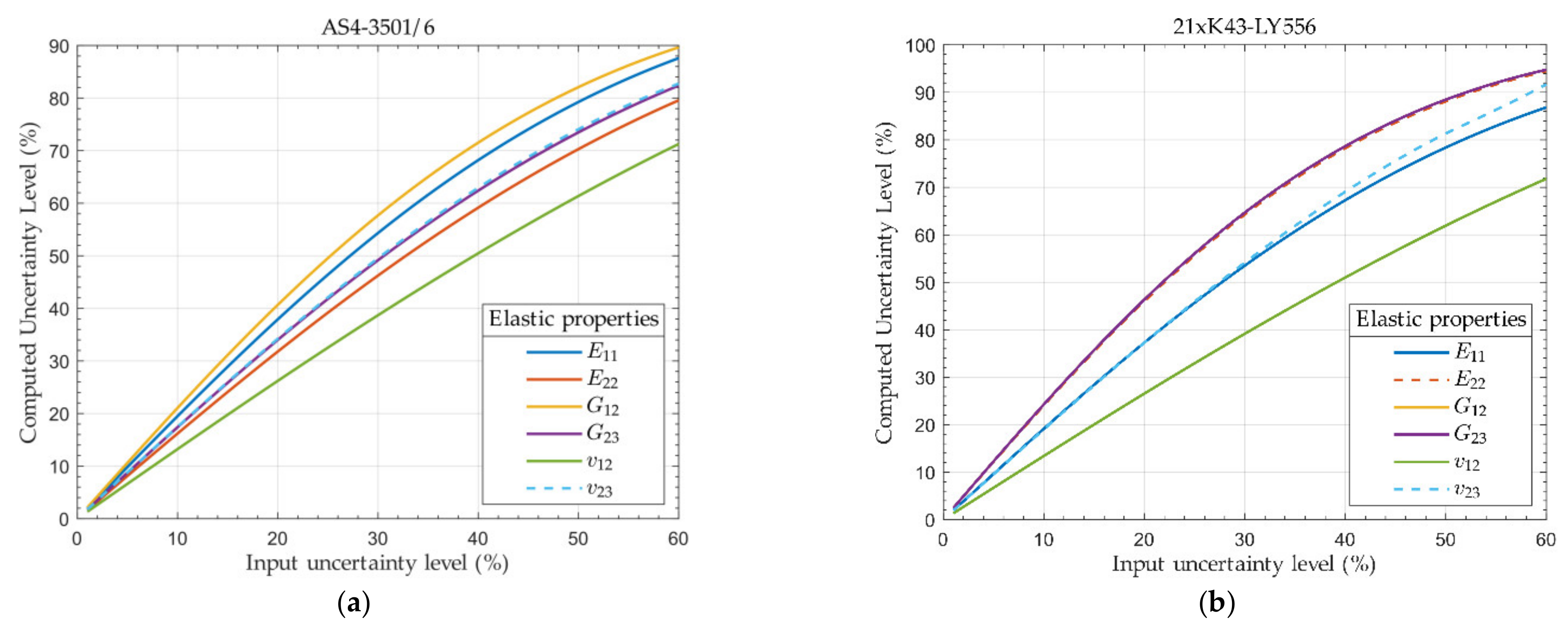
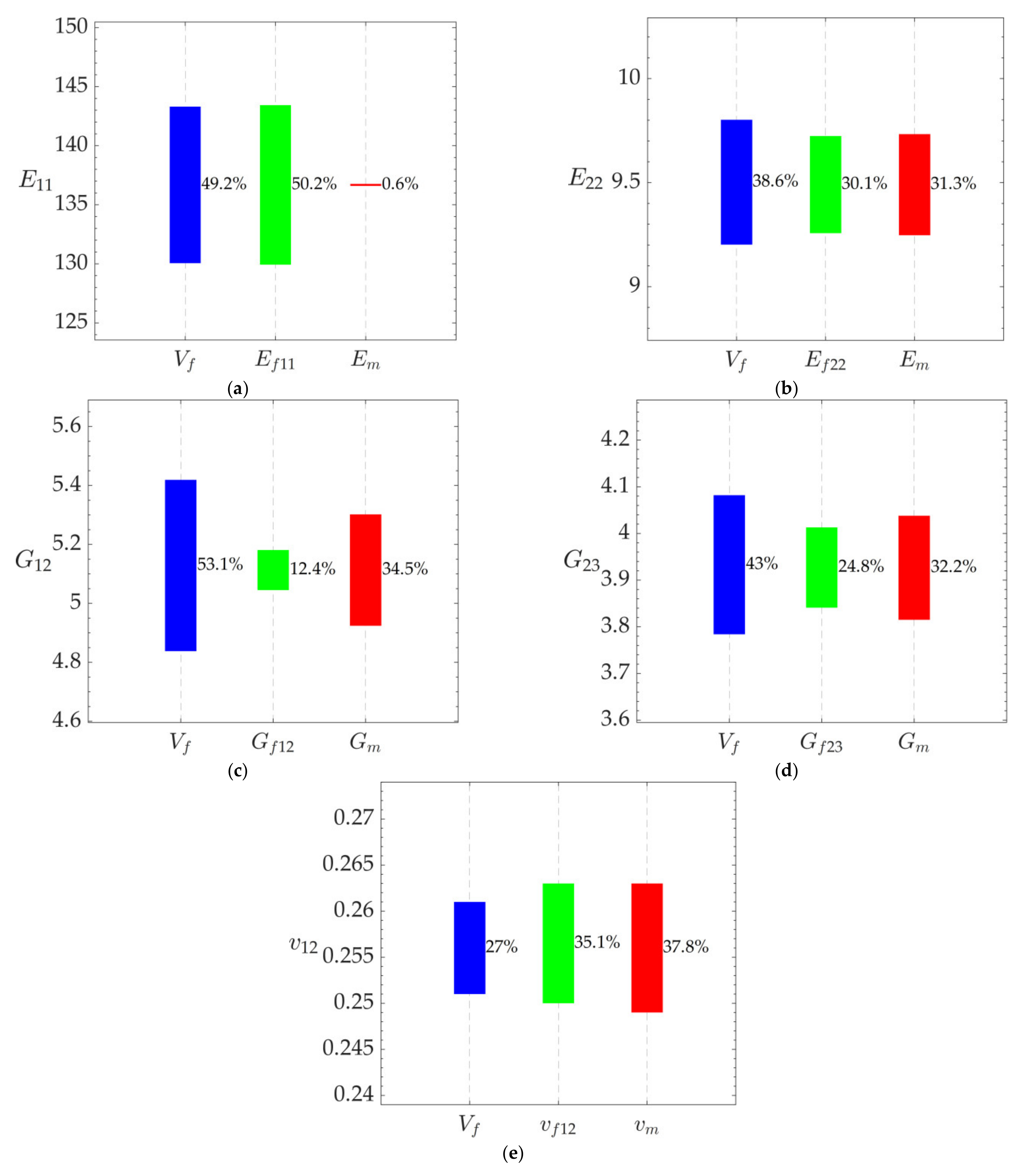
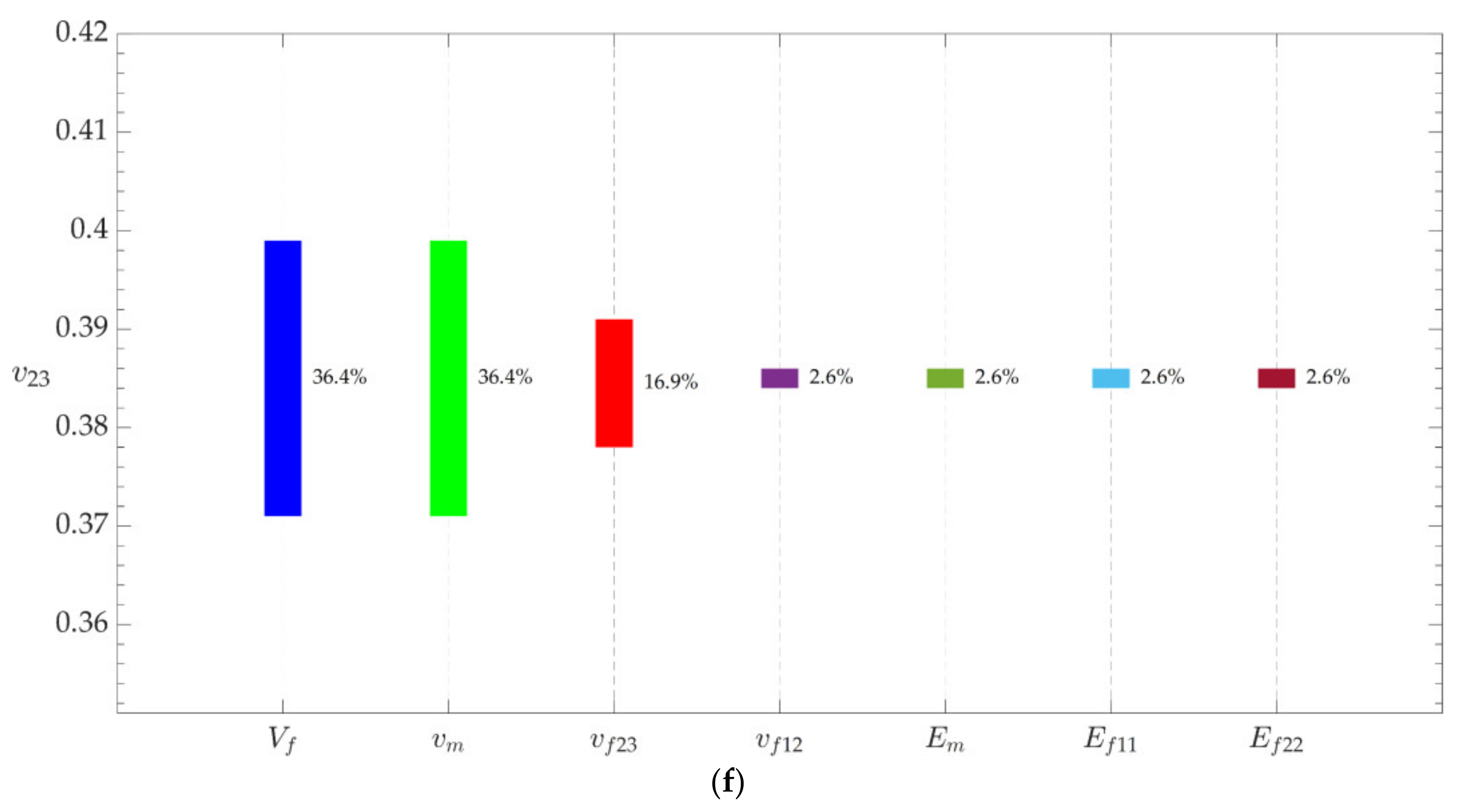
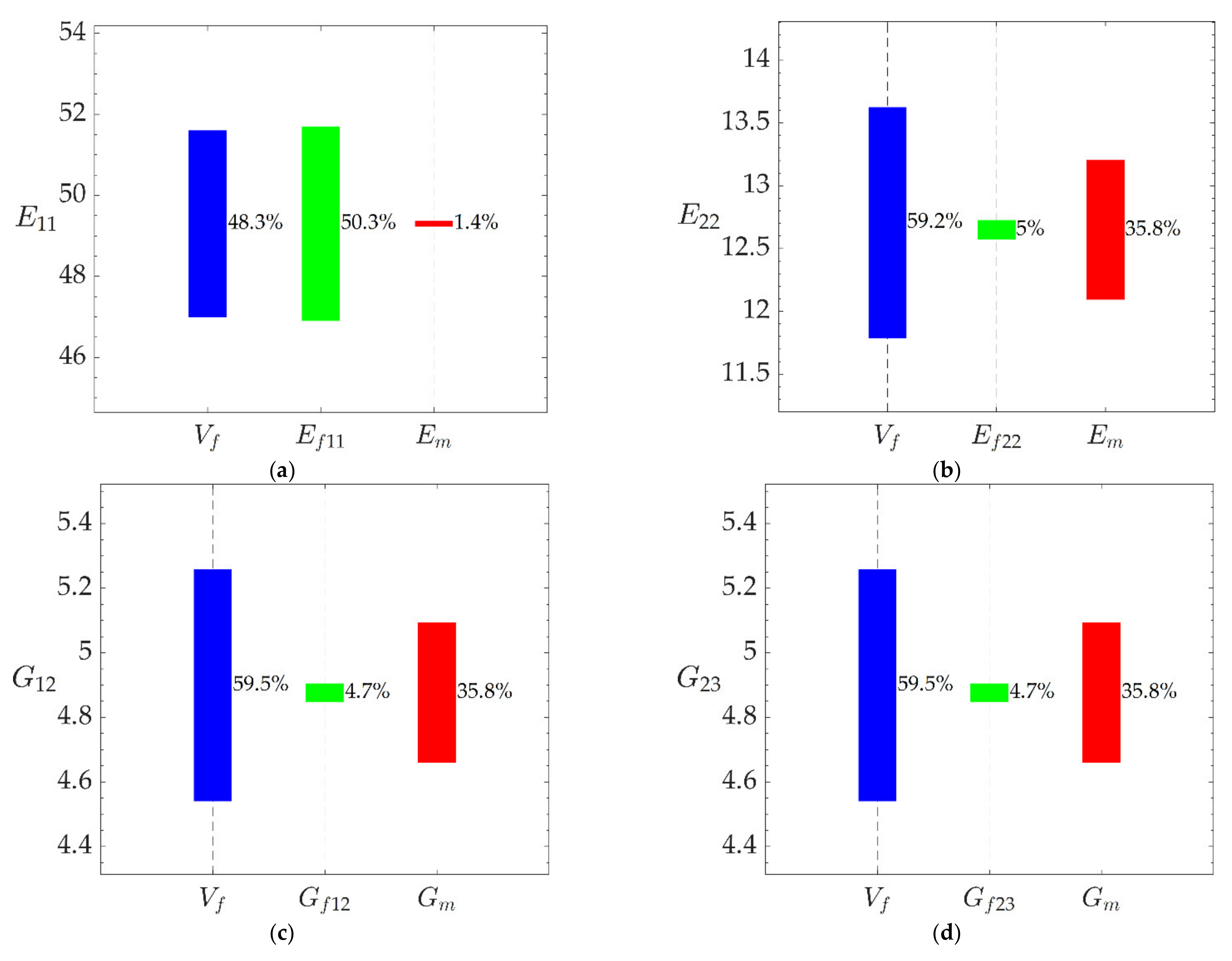
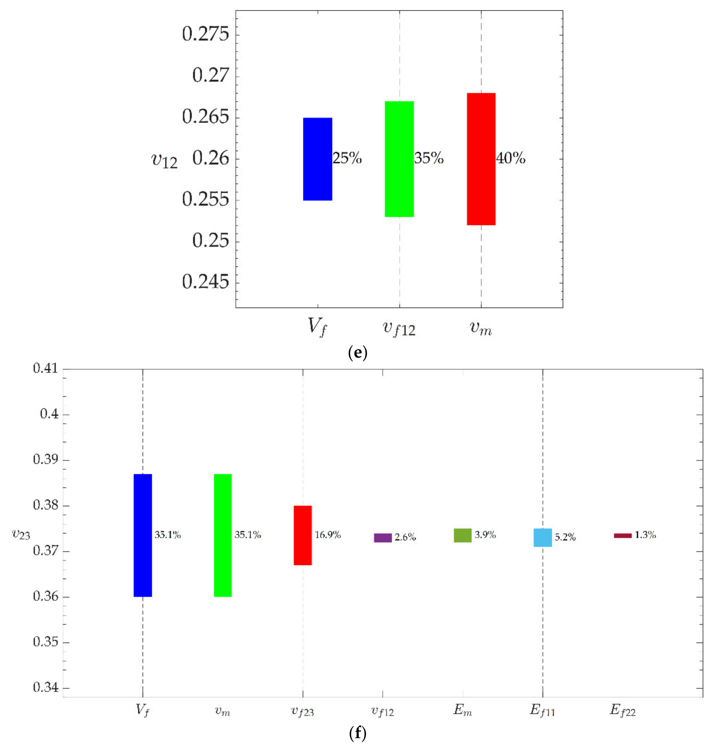
Sensitivity Analysis of the Elastic Properties

The uncertainties presented in Table 5 and Table 6 have been derived by considering an uncertainty of 5% for all properties of the constituent materials simultaneously. A piece of beneficial information is how the uncertainty of each input property contributes to the overall uncertainty of the elastic properties and strengths. In order to obtain this information, a sensitivity study of the elastic properties was performed by running analyses in which an uncertainty of 5% was used for a specific input property while the other input properties were kept equal to their nominal value. The results from the sensitivity study are shown in the bar charts of Figure 2 and Figure 3 for the two composite materials.

Figure 2. The effect of input parameters on the range of (a) the E₁₁, (b) the E₂₂, (c) the G₁₂, (d) the G₂₃, (e) the ν₁₂, and (f) the ν₂₃ for the AS4-3501/6 composite ply. The main parameter varied within ±5% of its nominal value while the other parameters were kept equal to the nominal value.

Figure 3. The effect of input parameters on the range of (a) the E₁₁, (b) the E₂₂, (c) the G₁₂, (d) the G₂₃, (e) the ν₁₂, and (f) the ν₂₃ for the 21xK43-LY556 composite ply. The main parameter varied within ±5% of its nominal value while the other parameters were kept equal to the nominal value.

Although, qualitatively, the contribution is the one expected from the mechanic’s viewpoint, it is very interesting to quantify it. For the AS4/3501-6 material, to the uncertainty of E₁₁, E_f11 contributes by 50.2% and V_f by 49.2%, with E_m by the minor 0.6%. To the uncertainty of E₂₂, V_f contributes by 38.6%; E_f22 by 30.1%; and E_m by 31.3%. To the uncertainty of G₁₂, V_f contributes by 53.1%; G_f12 by 12.4%; and G_m by 34.5%. To the uncertainty of G₂₃, V_f contributes by 43%; G_f23 by 24.8%; and G_m by 32.2%. To the uncertainty of ν₁₂, V_f contributes by 27%, ν_f12 by 35.1%; and ν_m by 37.8%. To the uncertainty of ν_f23, V_f contributes by 36.4%; ν_m by 36.4%; ν_f23 by 16.9%; and ν_f12, E_m, E_f11, and E_f22 by 2.6%. Similar values were obtained for the 21xK43-LY556 material (Figure 3). Similarly, for the strengths, to the uncertainty of F_1t, V_f contributes by 29.1%; F_ft by 50.2%; and F_mt by 0.7%; and to the uncertainty of F_1c, V_m contributes by 49.9% and V_m by 50.1.%. Similar values have been obtained for the 21xK43-LY556 material (Figure 3).

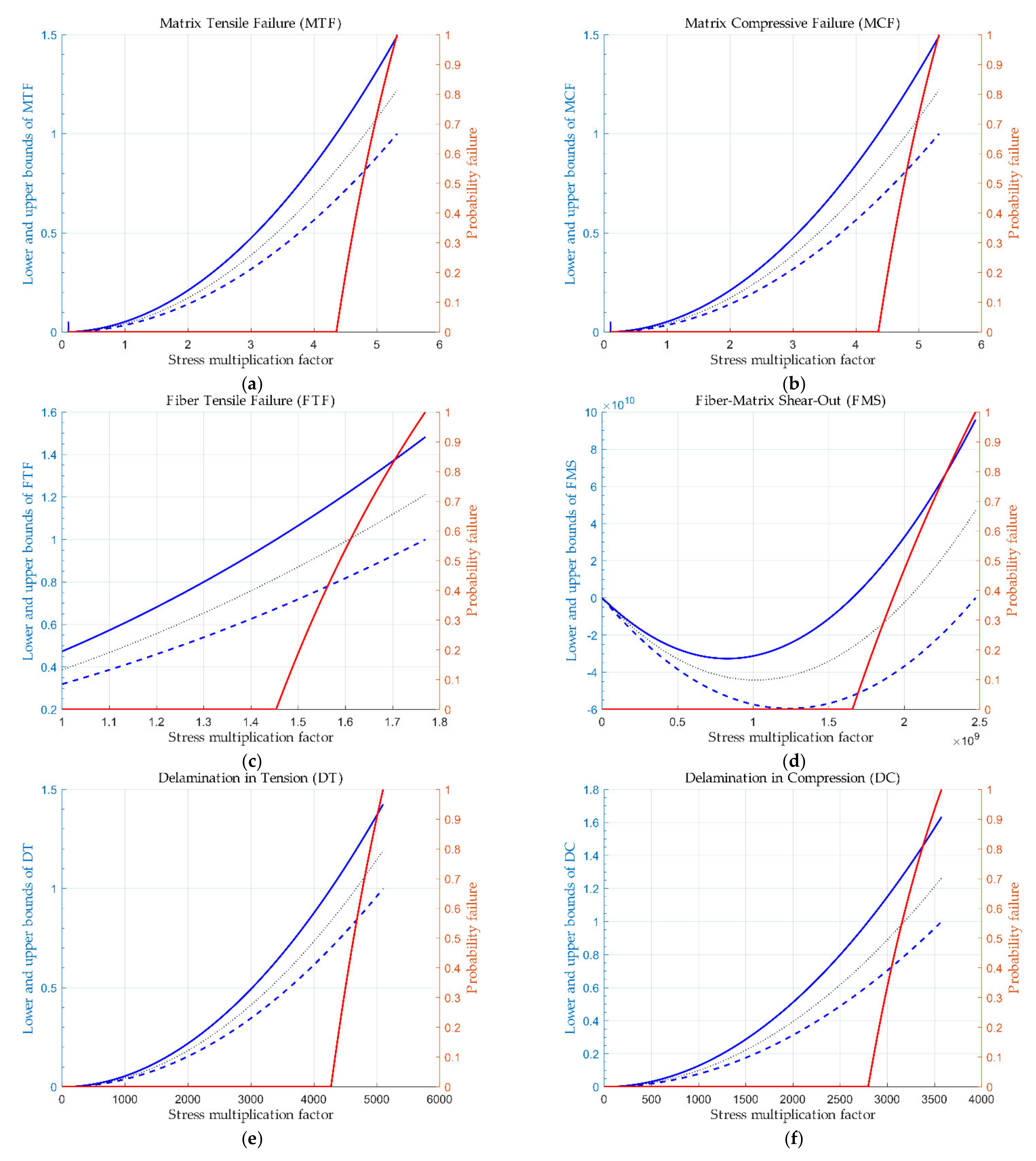
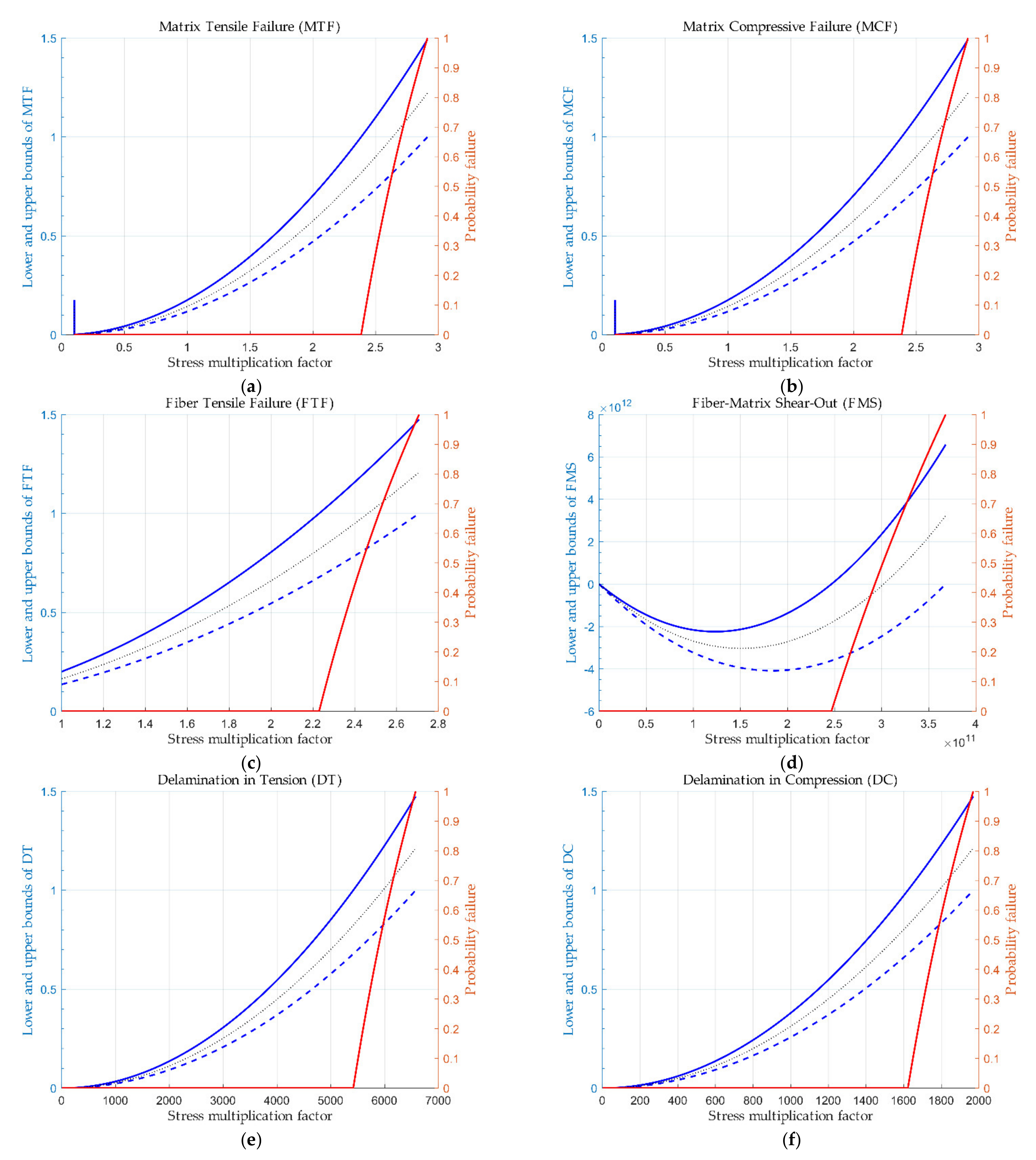
5. Uncertainty Computation in the Failure Assessment

Failure analysis of the UD ply was performed using the Hashin-type failure criteria [4]. Seven different failure modes were considered, namely, matrix tensile and compressive failure, fiber tensile and compressive failure, fiber-matrix debonding, and delamination in tension and compression. The mathematical expressions of the failure criteria are listed in Appendix B.

5.1. Methodology

This section exploits the computed bounds of the properties in connection with the Hashin-type failure criteria [4]. We can guarantee that, although there is uncertainty when the upper bound of a criterion is less than 1, there is no failure (100% safe). In different cases, we can quantify the failure probability. The same procedure can be applied to any other failure criteria, such as the Hoffman, Tsai-Wu, and Tsai-Hill criteria [16].

Here we demonstrate our approach using the matrix tensile failure criterion of Hashin

$$MTF\equiv \frac{{\sigma }_2^2}{F_{2t}^2}+\frac{{\sigma }_{12}^2+{\sigma }_{23}^2}{F_{12}^2}=1,\hspace{0.17em}\hspace{0.17em}{\sigma }_2>0$$

(5)

If we already know the ranges of $F_{2t}$ and $F_{12}$, we can express the left hand of Equation (5) using interval arithmetic operations, assuming that $0\notin F_{2t}^I=[\underset{¯}{F_{2t}},\overline{F_{2t}}]$ and $0\notin F_{12}^I=[\underset{¯}{F_{12}},\overline{F_{12}}]$, where the attached superscript “I” denotes the corresponding interval quantity. By taking the natural interval extension of $MTF$ and substituting the corresponding interval numbers $F_{2t}^I$ and $F_{12}^I$, we obtain

$$MT{F}^I=\left[\frac{{\sigma }_2^2}{{\overline{F_{2t}}}^2}+\frac{{\sigma }_{12}^2+{\sigma }_{13}^2}{{\overline{F_{12}}}^2},\frac{{\sigma }_2^2}{{\underset{¯}{F_{2t}}}^2}+\frac{{\sigma }_{12}^2+{\sigma }_{13}^2}{{\underset{¯}{F_{12}}}^2}\right]$$

in the endpoint coordinate system. Therefore, the lower bound is $a=\inf MT{F}^I$ and the upper bound $b=\sup MT{F}^I$. In addition, we can reformulate the interval $MT{F}^I$ in the midpoint-radius coordinate system as follows

$$\begin{array}{c}m\left(MT{F}^I\right)=\frac{1}{2}\left[{\sigma }_2^2\left(\frac{1}{{\underset{¯}{F_{2t}}}^2}+\frac{1}{{\overline{F_{2t}}}^2}\right)+\left({\sigma }_{12}^2+{\sigma }_{13}^2\right)\left(\frac{1}{{\underset{¯}{F_{12}}}^2}+\frac{1}{{\overline{F_{12}}}^2}\right)\right]\\ r\left(MT{F}^I\right)=\frac{1}{2}\left[{\sigma }_2^2\left(\frac{1}{{\underset{¯}{F_{2t}}}^2}-\frac{1}{{\overline{F_{2t}}}^2}\right)+\left({\sigma }_{12}^2+{\sigma }_{13}^2\right)\left(\frac{1}{{\underset{¯}{F_{12}}}^2}-\frac{1}{{\overline{F_{12}}}^2}\right)\right]\end{array}$$

where $r\left(MT{F}^I\right)$ represents the uncertainty of interval $MT{F}^I$ since $MT{F}^I=m\left(MT{F}^I\right)\pm r\left(MT{F}^I\right)$. After some algebraic manipulations, it is straightforward to derive the following formulae for the uncertainty of $MT{F}^I$.

$$r(MT{F}^I)=2{\sigma }_2^2\frac{r(F_{2t}^I)\hspace{0.33em}m(F_{2t}^I)}{{\left[m{(F_{2t}^I)}^2-r{(F_{2t}^I)}^2\right]}^2}+2\left({\sigma }_{12}^2+{\sigma }_{13}^2\right)\frac{r(F_{12}^I)\hspace{0.33em}m(F_{12}^I)}{{\left[m{(F_{12}^I)}^2-m{(F_{12}^I)}^2\right]}^2},$$

while its midpoint can also be calculated from the expression

$$m(MT{F}^I)={\sigma }_2^2\frac{m{(F_{2t}^I)}^2+r{(F_{2t}^I)}^2}{{\left[m{(F_{2t}^I)}^2-r{(F_{2t}^I)}^2\right]}^2}+\left({\sigma }_{12}^2+{\sigma }_{13}^2\right)\frac{m{(F_{12}^I)}^2+r{(F_{12}^I)}^2}{{\left[m{(F_{12}^I)}^2-r{(F_{12}^I)}^2\right]}^2}.$$

Hence, we derived the combined uncertainty in closed form explicitly. The expressions of the uncertainty of intervals for all Hashin-type failure criteria are reported in Appendix C.

Let $[a,b]$ be the range of values of a criterion under uncertainty; then, we define the probability of failure as:

$$P([a,b]\ge 1)=\left\{\begin{array}{ll}1,& a\ge 1\\ \frac{b-1}{b-a},& a<1\le b\\ 0,& b<1\end{array}\right.$$

(6)

5.2. Results

The effect of the uncertainty in the strengths of the UD lamina on the efficiency of the failure analysis has been studied based on a UD composite laminated plate subjected to quasi-static tension. The plate dimensions are 250 mm × 25 mm × 2 mm, and the lay-up is [0/45/90-45]_2S. The stress analysis of the plate was performed using the ANSYS FE software and the SOLID185 element. In order to model the tensile load, an axial displacement of 2.5 mm (1% strain) was applied at the nodes of one end while the nodes of the other end were kept fully fixed. The computed stresses for each lamina, used as input to the failure criteria, are listed in Table 10. They were taken at the middle point of the plate. It is noted that, since the input stresses were used only for demonstrating the computational method for the uncertainty of the failure analysis, the FE model was neither optimized nor validated.

Table 10. Input stresses (MPa) are computed by the FE model.

Layer	${\mathit{\sigma }}_1$	${\mathit{\sigma }}_2$	${\mathit{\sigma }}_3$	${\mathit{\sigma }}_{12}$	${\mathit{\sigma }}_{23}$	${\mathit{\sigma }}_{13}$
0°	1138.460	0.510	0.026	−18.250	−0.210	0.030
45°	231.886	114.404	−0.054	128.684	0.029	−0.030
90°	102.376	−341.169	−0.004	−18.250	0.029	−0.044
−45°	231.820	114.404	−0.014	−165.185	0.013	−0.044
0°	1138.460	0.510	0.026	−18.250	0.042	−0.044
45°	231.886	114.404	−0.054	128.684	0.042	−0.044
90°	102.376	−341.169	−0.004	−18.250	0.042	0.004
−45°	2318.820	114.404	−0.014	−165.185	0.042	0.013

The uncertainty in the assessment of the first ply failure was computed. Seven failure modes have been considered, namely:

• Matrix Tensile Failure (MTF);
• Matrix Compressive Failure (MCF);
• Fiber Tensile Failure (FTF);
• Fiber Compressive Failure (FCF);
• Fiber-Matrix Shear-Out (FMS);
• Delamination in Tension (DT);
• Delamination in Compression (DC).

Given that neither material nor geometrical nonlinearity is present, a linear variation of stresses with the applied load is assumed. Therefore, for the developed stresses to cause failure, a stress multiplication factor was applied instead of load increase.

Figure 4 and Figure 5 plot the variation in the lower and upper bounds and the nominal value of the six failure criteria (Equations (A13), (A14), (A15), (A17), (A18), (A19)) as well as the probability of failure (Equation (6)) of each failure mode with regards to the stress multiplication factor for the two UD composite plies. Note that the fiber compressive failure mode has been excluded since it is not a feasible failure mode for a ply under tension; σ₁ is always positive. The very large values of the stress multiplication factor appear for delamination because, for the specific loading (uniaxial tension), delamination is very difficult to develop; it is almost not feasible. As long as the upper bound of the failure criteria remains below 1.0, the probability of failure is 0. When the upper bound exceeds 1.0, the probability of failure starts to increase linearly at a high slope.

Figure 4. Plots of the upper and lower bounds, the nominal value of failure criteria, and the probability of failure regarding the stress multiplication factor for the AS4-3501/6 UD ply.

Figure 5. Plots of the upper and lower bounds, the nominal value of failure criteria, and the probability of failure regarding the stress multiplication factor for the 21xK43-LY556 UD ply.

Table 11 lists the values plotted in the diagram of Figure 4 for the matrix tensile failure for a range of stress multiplication factors between 4.35 and 5.32. It is shown that, for nominal values above 0.9, for which classical analysis means no failure, there is a probability of failure of more than 30%. For nominal values more than 0.95, the probability of failure exceeds 40%.

Table 11. Variation in the interval parameters and the probability of failure regarding the stress multiplication factor for the MTF. The bold number in the 3rd column corresponds to the first value of the failure criterion above 1.0 (failure) and the coloring of the values in the last column correspond to different intensity ranges of the probability of failure; the intensity increases from green to dark red.

Stress Multiplication Factor	Lower Bound	Nominal Value of the Failure Criterion	Upper Bound	Probability of Failure
4.351535	0.66887	0.817096	0.99817	0.0%
4.400102	0.683884	0.835437	1.020575	6.1%
4.500221	0.71536	0.873888	1.067548	19.2%
4.600318	0.747537	0.913196	1.115566	31.4%
4.700291	0.78038	0.953318	1.164579	42.8%
4.800035	0.813852	0.994208	1.214531	53.5%
4.900427	0.848251	1.036229	1.265865	63.7%
5.000417	0.883221	1.078948	1.31805	73.1%
5.100407	0.918896	1.122529	1.371289	82.1%
5.200316	0.955248	1.166937	1.425538	90.5%
5.300061	0.992244	1.212132	1.480748	98.4%
5.320771	1.000013	1.221623	1.492343	100.0%

6. Conclusions

In the present paper, an interval-based method was presented to compute the uncertainty in the computed mechanical properties and the failure analysis of composite unidirectional (UD) laminates. The method was applied to two composite materials: the carbon/epoxy AS4-3501/6 and the glass/epoxy 21xK43-LY556. An uncertainty level of 5% was assumed for the input properties of the constituents (fibers and matrix).

The computed uncertainty level for the mechanical properties ranges from 6.64% to 10.63% for the AS4-3501/6 material and from 6.72% to 12.28% for the 21xK43-LY556 material. For evaluating the uncertainty effect on the efficiency of failure criteria, a probability of failure function has been defined. The probability is zero until the upper bound of the failure criteria becomes 1.0. From that point, it increases linearly at a high slope. Indicative of the uncertainty in the efficiency of failure criteria is that, for nominal values equal to 0.9, the probability of failure is above 30%, and for values close to 0.990 it is above 50%.

The present work demonstrates the potential of interval arithmetic for problems from materials science and mechanics. The authors intend to perform the uncertain assessment using realistic input uncertainty values coming from tests as a future step.

References

- Pantelakis, S.; Tserpes, K. (Eds.) Revolutionizing Aircraft Materials and Processes; Springer International Publishing: Cham, Switzerland, 2020; ISBN 978-3-030-35345-2. [Google Scholar]
- Chamis, C. Simplified Composite Micromechanics Equations for Strength, Fracture Toughness, Impact Resistance and Environmental Effects; Lewis Research Center, National Aeronautics and Space Administration: Cleveland, OH, USA, 1984.
- Hinton, M.; Soden, P.; Kaddour, A.-S. Failure Criteria in Fibre-Reinforced-Polymer Composites; Elsevier: Amsterdam, The Netherlands, 2004; ISBN 978-0-08-044475-8. [Google Scholar]
- Hashin, Z. Failure Criteria for Unidirectional Fiber Composites. J. Appl. Mech. 1980, 47, 329–334. [Google Scholar] [CrossRef]
- Tserpes, K.I.; Papanikos, P.; Kermanidis, T. A Three-Dimensional Progressive Damage Model for Bolted Joints in Composite Laminates Subjected to Tensile Loading: Failure of tensile-loaded bolted composite joints. Fatigue Fract. Eng. Mater. Struct. 2001, 24, 663–675. [Google Scholar] [CrossRef]
- Tserpes, K.I.; Labeas, G.; Papanikos, P.; Kermanidis, T. Strength Prediction of Bolted Joints in Graphite/Epoxy Composite Laminates. Compos. Part B Eng. 2002, 33, 521–529. [Google Scholar] [CrossRef]
- Kolks, G.; Tserpes, K.I. Efficient Progressive Damage Modeling of Hybrid Composite/Titanium Bolted Joints. Compos. Part Appl. Sci. Manuf. 2014, 56, 51–63. [Google Scholar] [CrossRef]
- Stamopoulos, A.G.; Tserpes, K.I.; Dentsoras, A.J. Quality Assessment of Porous CFRP Specimens Using X-Ray Computed Tomography Data and Artificial Neural Networks. Compos. Struct. 2018, 192, 327–335. [Google Scholar] [CrossRef]
- Murthy, P.L.N.; Mital, S.K.; Shah, A.R. Probabilistic Micromechanics/Macromechanics for Ceramic Matrix Composites. J. Compos. Mater. 1998, 32, 679–699. [Google Scholar] [CrossRef]
- Stock, T.A.; Bellini, P.X.; Murthy, P.L.; Chamis, C.C. A Probabilistic Approach to Composite Micromechanics. In Proceedings of the 29th Structures, Structural Dynamics and Materials Conference, Williamsburg, VA, USA, 18–20 April 1988. [Google Scholar]
- Chen, N.; Yu, D.; Xia, B.; Liu, J.; Ma, Z. Interval and Subinterval Homogenization-Based Method for Determining the Effective Elastic Properties of Periodic Microstructure with Interval Parameters. Int. J. Solids Struct. 2017, 106–107, 174–182. [Google Scholar] [CrossRef]
- Wang, L.; Wang, X.; Su, H.; Lin, G. Reliability Estimation of Fatigue Crack Growth Prediction via Limited Measured Data. Int. J. Mech. Sci. 2017, 121, 44–57. [Google Scholar] [CrossRef]
- Wang, L.; Liu, D.; Yang, Y.; Wang, X.; Qiu, Z. A Novel Method of Non-Probabilistic Reliability-Based Topology Optimization Corresponding to Continuum Structures with Unknown but Bounded Uncertainties. Comput. Methods Appl. Mech. Eng. 2017, 326, 573–595. [Google Scholar] [CrossRef]
- Alazwari, M.A.; Rao, S.S. Modeling and Analysis of Composite Laminates in the Presence of Uncertainties. Compos. Part B Eng. 2019, 161, 107–120. [Google Scholar] [CrossRef]
- Alazwari, M.A.; Rao, S.S. Interval-Based Uncertainty Models for Micromechanical Properties of Composite Materials. J. Reinf. Plast. Compos. 2018, 37, 1142–1162. [Google Scholar] [CrossRef]
- Rao, S.S.; Alazwari, M.A. Failure Modeling and Analysis of Composite Laminates: Interval-Based Approaches. J. Reinf. Plast. Compos. 2020, 39, 817–836. [Google Scholar] [CrossRef]
- Moore, R.E.; Kearfott, R.B.; Cloud, M.J. Introduction to Interval Analysis; Society for Industrial and Applied Mathematics: Philadelphia, PA, USA, 2009; ISBN 978-0-89871-669-6. [Google Scholar]
- Hansen, E.R.; Walster, G.W. Global Optimization Using Interval Analysis. In Monographs and Textbooks in Pure and Applied Mathematics, 2nd ed.; Revised and Expanded; Marcel Dekker: New York, NY, USA, 2004; ISBN 978-0-8247-4059-7. [Google Scholar]
- Ratschek, H.; Rokne, J. Computer Methods for the Range of Functions; Ellis Horwood Series in Mathematics and Its, Applications; Horwood, E., Ed.; Halsted Press: Chichester, UK; New York, NY, USA, 1984; ISBN 978-0-85312-703-1. [Google Scholar]
- Krämer, W. High Performance Verified Computing Using C-XSC. Comput. Appl. Math. 2013, 32, 385–400. [Google Scholar] [CrossRef]
- Kulisch, U.; Hammer, R.; Hocks, M.; Ratz, D. C++ Toolbox for Verified Computing I; Springer: Berlin/Heidelberg, Germany, 1995; ISBN 978-3-642-79653-1. [Google Scholar]
- Caprani, O.; Madsen, K. Mean Value Forms in Interval Analysis. Computing 1980, 25, 147–154. [Google Scholar] [CrossRef]
- Rall, L.B. Mean Value and Taylor Forms in Interval Analysis. SIAM J. Math. Anal. 1983, 14, 223–238. [Google Scholar] [CrossRef]
- Baumann, E. Optimal Centered Forms. BIT 1988, 28, 80–87. [Google Scholar] [CrossRef]
- Sotiropoulos, D.G.; Grapsa, T.N. Optimal Centers in Branch-and-Prune Algorithms for Univariate Global Optimization. Appl. Math. Comput. 2005, 169, 247–277. [Google Scholar] [CrossRef]
- Ratz, D. Automatische Ergebnisverifikation Bei Globalen Optimierungsproblemen. Ph.D. Dissertation, Universität Karlsruhe (TH), Institute for Applied Mathematics, Karlsruhe, Germany, 1992. [Google Scholar] [CrossRef]
- Ratz, D.; Csendes, T. On the Selection of Subdivision Directions in Interval Branch-and-Bound Methods for Global Optimization. J. Glob. Optim. 1995, 7, 183–207. [Google Scholar] [CrossRef]
- Soden, P. Lamina Properties, Lay-up Configurations and Loading Conditions for a Range of Fibre-Reinforced Composite Laminates. Compos. Sci. Technol. 1998, 58, 1011–1022. [Google Scholar] [CrossRef]
Publisher’s Note: MDPI stays neutral with regard to jurisdictional claims in published maps and institutional affiliations. |
© 2022 by the authors. Licensee MDPI, Basel, Switzerland. This article is an open access article distributed under the terms and conditions of the Creative Commons Attribution (CC BY) license (https://creativecommons.org/licenses/by/4.0/).