Abstract
In this paper, we propose a method for semi-supervised image segmentation based on geometric active contours. The main novelty of the proposed method is the initialization of the segmentation process, which is performed with a polynomial approximation of a user defined initialization (for instance, a set of points or a curve to be interpolated). This work is related to many potential applications: the geometric conditions can be useful to improve the quality the segmentation process in medicine and geophysics when it is required (weak contrast of the image, missing parts in the image, non-continuous contour…). We compare our method to other segmentation algorithms, and we give experimental results related to several medical and geophysical applications.
1. Introduction
The problem of segmenting an image into its significant components has been studied for over 30 years in computers science, applied mathematics and more generally in computer vision.
Recently, from convolutional neural networks (see Fukushima [1], Waibel et al. [2], and LeCun et al. [3], among others…) to recurrent neural networks (Hochreiter and Schmidhuber [4]), encoder–decoders (Badrinarayanan et al. [5]), or generative adversarial networks (Goodfellow et al. [6]), deep learning based techniques have achieved huge successes in the field of artificial intelligence and image segmentation (see [7] for a recent survey). These approaches leads to excellent results, including in medical applications (see for example Fantazzini et al. [8]). However, in general, the performance heavily depends on labeled data, and this point is a main difficulty on several applications when lacking labeled data such as in many medical and geophysical applications. The data augmentation is possible [9], but it is often complicated, and requires more CPU/GPU time than other segmentation techniques based on energy minimization or variational approaches (Kass et al. [10], Chand and Vese [11], Mumford and Shah [12], Vese and Le Guyader [13]…) or geometrical ones (fast marching methods, see Sethian [14] or Forcadel et al. [15]).
In this work, we focus on a modeling based on a variational approach: it basically consists of evolving an initial contour subject to constraints towards the boundary of the object to be detected. This deformation is done by minimizing a functional depending on the curve and defined so that a local minimum is obtained at the boundary of the object. This energy-like functional minimization problem has led to many research works in the last 25 years. Caselles, Kimmel and Sapiro [16] have shown that by setting one of the regularization parameters to zero in the classical active contour model, one gets a problem equivalent to finding a geodesic curve in a Riemann space whose metric depends on the image contents. The issue was then no longer seen as an energy-like minimization problem but as a curve evolution one. Let us note that this approach is very suitable to our problems, and it could be possible to use deep learning (DL) based algorithm (as used by Le Guyader et al. [17]), but the a priori conditions are complicated to integrate in such DL models (and such DL models require a lot of hardware, much more that our proposed algorithm).
An edge can be viewed as the locus of connected points for which the image gradient varies abruptly. However, when data acquisition cannot be performed in an optimal manner (e.g., liver in medical imaging), this criterion can no longer be applied. In many applications, image data are missing or of poor quality, and occultation phenomena can often occur: two objects that are adjacent to one another can own intrinsic homogeneous textures so that it is hard to clearly identify the interface between them. It is then relevant to introduce geometric constraints in the modeling to help the segmentation process. In [18,19,20,21], the authors introduce the concept of a finite set of points to be interpolated during the segmentation process (like in Gout and Le Guyader [20]) or a variational approach to integrate higher-level shape priors into level set based segmentation method (see Cremers et al. [18]). However, in some applications (in geophysics or in several medical applications), this is not sufficient and adding new a priori conditions to be satisfied is required both to improve the segmentation process and also to simplify the initial condition (in [20], the method requires a priori conditions plus an initial guess to start the segmentation process, which constitutes a drawback of their algorithm).
In this work, we propose to consider a curve (or a set of curves) belonging to the searched contour of interest, integrated as an initial condition to be satisfied by the final segmentation contour obtained at the end of the segmentation process. This is an added value considering previous models (like [19]), where it was necessary to both give an initial condition and geometric conditions. In order to define this curve, it is possible to use -spline functions (see Gout et al. [22]) obtained by minimizing an energy functional on a suitable Hilbert space (and so a set of points given by the user is sufficient to create such geometric conditions).
In this paper, we generalize and improve the approach of Gout and Le Guyader [20]: we combine the curve evolution approach developed by Caselles, Kimmel and Sapiro [16], with a geometrical approach consisting in a curve given by the user (a set of points can also be considered like in Gout and Le Guyader [20]), and the initial condition is then automatically generated (from the geometric conditions).
In Section 2, we give the modeling of our problem, based on a level set method (LSM) approach (Osher and Sethian [23], see also [24]). Using Euler-Lagrange variational principle, we obtain the PDE satisfied by the 3D LSM function and the corresponding evolution problem is then given. The existence and uniqueness of the viscosity solution of the associated parabolic problem is also established: we give the main steps of the proof (based on Caselles et al. [16] and Gout and Le Guyader [20]). The discretization of the problem is tackled in Section 3, and is solved using an Additive Operator Splitting scheme (Weickert and Kühne [25]). Comparisons and experimental results with the proposed approach are given for several medical and geophysical imaging applications.
2. Mathematical Modelling
The well-known level set approach (see Osher and Sethian [23]) consists in considering the evolving active contour as the zero level set of a function , which is a Lipschitz continuous function defined by:
such that:
and takes opposite signs on each side of . This level set approach enables us to re-write the energy in terms of :
where H is the one-dimensional Heaviside function and where . We formulate the shape optimization problem as follows: “Find a shape such that the energy E is minimized”:
The functional E being not Gâteaux-differentiable, we regularize the problem by considering slightly regularized versions ( or regularization) of the functions H and (the one dimensional Dirac measure) denoted, respectively, by and , and considering that , the associated regularized functional becomes:
where:
is an approximation of the length of the zero level set of .
2.1. A Priori Conditions
We now propose to include a priori condition in the process. We consider the a priori condition as a smooth arc curve given by the user. The curve is parametrised by . By construction, we impose that the curve belongs to the level set . The first step consists in constructing the initial condition from the geometric conditions given by the user. We have chosen this option, because it permits to avoid the stage of giving an initial condition plus the a priori conditions.
The first step consists in closing the arc to get a closed curve. We introduce a point and a vector It is easy to construct two (unique) polynomials curves and that are parameterized using and such that:
We set and we consider as the signed distance to
To define the energy we also introduce the mask : IR:
where IR is a positive parameter which controls the width of the mask. Then, we can define the following energy functional:
The goal is to minimize the norm between and : we impose the contour to be close to The mask permits to impose such influence in (and only in) a local neighborhood of .
2.2. Minimization Problem and Evolution Equation
The modeling of our problem consists in minimizing the energy:
with
We now give the evolution problem. We minimize with respect to and deduce the associated Euler–Lagrange equation for :
with the boundary conditions (homogeneous Neumann):
denoting the exterior normal to the boundary of
When a local minimum is reached, then the quantity tends to 0, which means that the steady state is reached. A rescaling can be made so that the motion is applied to all level sets by replacing by (It makes the flow independent of the scaling of ).
Let us also note that the speed of convergence of the model can be increased by adding the component in the evolution equation, being a constant. This component can be seen as an area constraint. An analogy with the Balloon model developed by Cohen [26] can be made: this constant motion term prevents the curve from stopping on a non-significative local minimum and is also of importance when initializing the process with a curve inside the object to be detected.
Thus, the proposed parabolic problem with the associated boundary conditions can be written:
2.3. Existence, Uniqueness of the Solution
This section is a theoretical part showing the existence and uniqueness of the solution of our segmentation model. We can show the existence and uniqueness of a viscosity solution to the evolution problem (14). We rewrite our problem as:
where, for :
and:
We assume that is a bounded domain in with a boundary. Under the following conditions, the Equation (15) has a unique viscosity solution.
- where denotes the space of symmetric matrices equipped with the usual ordering.
- There exists a constant such that for each:the function:is non-decreasing on .
- For each , there exists a continuous function satisfying such that if and satisfy:then:for all with and .
- For each , the function is positively homogeneous of degree one in p, i.e., , .
- There exists a positive constant such that for all and . Here, denotes the unit outer normal vector of at
All those conditions are clearly satisfied for , and B (see for instance [20]). We here have to extend the proof to .
- Thanks to [20], we already know that . Since, , it is clear that and therefore .
- Note that since F does not depend on u. It suffices to show that is non-decreasing on . On can easily see that the condition is satisfied for all as soon as .
- Since g does not depend on X, it suffices to check the condition on F. We refer the reader to Gout and Le Guyader [20] for the proof.
The proof for conditions 4–6 are basic, and can be found for instance in [20]. Therefore, all the conditions are satisfied and the evolution problem (14) has a unique viscosity solution.
3. Experimental Results
For the discretization scheme, we use the additive operator splitting scheme (AOS) proposed by Weickert and Kuhne ([25], see also [20]). This corresponding algorithm requires a computational cost linear in (size of the unknown vector ) at each step. This scheme is well-suited to our problem that differs only in the introduction of the function .
We use the method proposed in this paper knowing that:
- –
- Following the considered application, the initial condition can be a set of points, or a curve (then can be constructed from a set points using a basic spline function (see Gout et al. [22])).
- –
- The stop criterion can be either a preset number of iterations or a check that the solution is stationary.
- –
- The distance is normalized in order to have the same weight between a priori information of the image and geometrical constraints.
- –
- The discretization is made using finite differences as done in Chan and Vese [11].
- –
- In the numerical examples, we take , the regularization term is equal to 0.8.
To illustrate the interest of our approach, we start with a simple test case, using a three-band image. Then, we run the method on blood vessel image. We obtain the following results. Without a priori condition, the segmentation process will of course give the entire white band as a result. This is the interest of adding such a priori condition to enforce the contour to arbitrary stop following the choice of the user.
We can see that the final contour correctly takes into account the curve given by the user imposing a constraint independent of the pixel values of the images, and correctly segment the white zone.
Of course, our approach allows us (to help) the segmentation process on “complicated” images, when ground truth informations are required like in Figure 1 or in many other cases, especially in geophysical or medical imaging. In Section 3.1, we illustrate the added value brought by our approach considering the initial guess choice improvement. Two examples are given to show that, compared to Gout et al. method [19], the approach given in this paper is much faster to get the same result since the initial guess is (strongly) optimized.
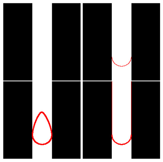
Figure 1.
Three-band image (top left), user-defined constraint (top right), initial contour automatically defined by our approach (bottom left) and final contour (bottom right).
In Section 3.2, we propose to compare our approach with well-known algorithms (Chan-Vese [11], U-Net [27]).
In Section 3.3 and Section 3.4, we give experimental results in medicine and geophysics.
3.1. Impact of the Initial Guess on the Segmentation Process
In this part, we focus on the added value brought by the automatic initial guess we propose, obtained from the geometrical condition given by the user. We compare our approach to the one introduced by Gout, Le Guyader and Vese [19], we take the same geometrical conditions, and then compare the number iteration to get the same final contour. The comparison is relevant because the segmentation algorithm is analogous in the two considered methods. In [19], note that we have to add a closed contour to the geometric conditions to start the segmentation process, while our proposed approach leads to an automatic initial guess (obtained from the geometric conditions given by the user). In the following two numerical examples, we take exactly the same interpolation conditions (3 points).
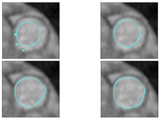
Figure 2.
We use Gout et al. [19] algorithm. The initial guess is given inside the region of interest, it is defined by , the time step is equal to 0.6, space step is equal to 0.1, distance is computed using the fast marching method (Sethian [14]) and the regularization term is equal to 0.8. Top left: Interpolation condition and initial closed contour. Top right: iteration 120. Bottom left: Iteration 240. Bottom right: Iteration 420.
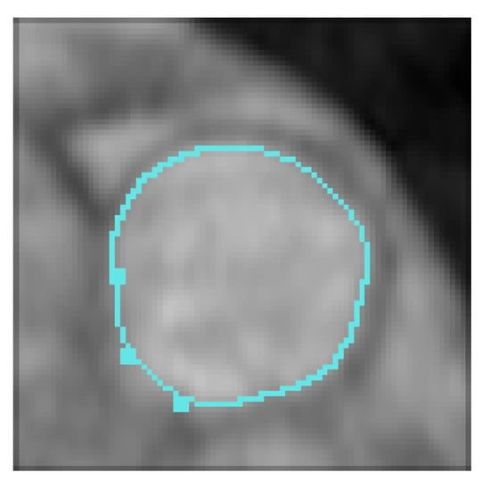
Figure 3.
Final result (iteration 420), with the interpolation conditions (3 points) using Gout et al. algorithm [19].
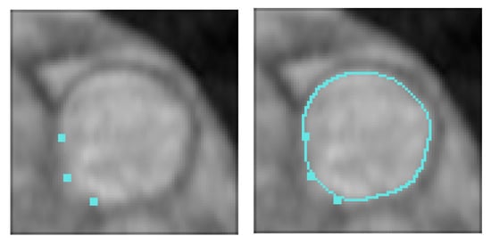
Figure 4.
Using our proposed approach, the process does not require an initial guess, the interpolation conditions automatically initiate the process. Left: interpolation conditions. Right: final result after 80 iterations.
We repeat the same process in the following example (Figure 5, Figure 6 and Figure 7). The initial contour for Gout et al. [19] algorithm is here chosen outside the region of interest. Of course, we take exactly the same interpolation conditions (3 points) in both cases.

Figure 5.
We use Gout et al. [19] algorithm. The initial guess is given outside the region of interest, it is defined by , the time step is equal to 0.3, space step is equal to 0.1, distance is computed using the fast marching method (Sethian [14]) and the regularization term is equal to 0.8. Top left: Interpolation condition and initial guess. Top right: iteration 80. Bottom left: Iteration 100. Bottom right: Iteration 160.
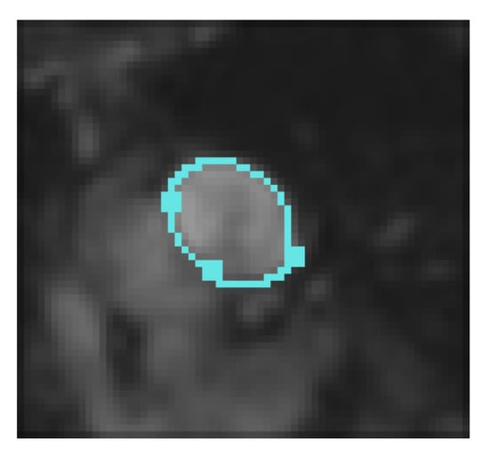
Figure 6.
Final result (iteration 260), with the interpolation conditions (3 points) using Gout et al. algorithm [19].
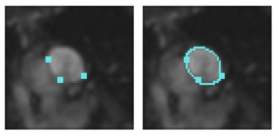
Figure 7.
Left: interpolation conditions. Right: final result after 8 iterations using our proposed approach.
In the example given on Figure 5, Figure 6 and Figure 7, we can see that our approach requires 30 times less iterations.
In this subsection, we illustrate the gain of the automatic generated initial guess we propose from the geometric conditions (see Table 1).

Table 1.
Gain of the automatic generated initial guess.
To get the same final contour, our method clearly requires much less iterations. This result is analogous on all the tests we have done, especially when a closed contour is chosen outside the region of interest (in [19]), in this case, the total number of iterations is reduced by a factor of 5 to 60. If the initial contour in [19] is chosen inside the region of interest, the total number of iterations is reduced by a factor of 4 to 20. The only cases where the number of iterations is equivalent between the two different methods are when we choose as initial guess in [19] a closed curve very close to the final result and interpolating at least 2 given interpolation conditions, this is of course a major constraint.
3.2. Quantitative Performance
We use the BraTS Dataset [28], which was collected and shared by the MICCAI Brain Tumor Segmentation Challenge (see [28] for more details) several years ago. We use 270 MR scans, each with four MIR sequences: T1-weighted (native image, sagittal or axial 2D acquisitions with 1–6 mm slice thickness), T1-weighted with contrast-enhanced (Gadolinium) image, T2-weighted image (axial 2D acquisition, with 2–6 mm slice thickness), and FLAIR (T2-weighted FLAIR image, axial, coronal, or sagittal 2D acquisitions, 2–6 mm slice thickness) (see [28] for more details). The training data have the size pixels, and have the manual segmentation labels for many types of brain tumors. We trained the network to generate segmentation masks corresponding to the center slice of the input. We used the well-known Adam optimization method [29]. We trained the deep network using 238 training data, we set the initial learning rate as , and multiplied by 0.5 after every 20 epochs. Using a single GPU, we trained the models with batch size 4 for 40 epochs.
In order to evaluate the performance of our method, we give comparisons between several algorithms. We here recall several metrics:
- –
- The Jaccard index [30], or Intersection over Union (IoU), is a commonly used metric in segmentation. It is defined as the area of intersection between the predicted segmentation map and the ground truth, divided by the area of union between the predicted segmentation map and the ground truth:where G is the ground truth and P denotes the predicted segmentation maps. It ranges between 0 and 1. Mean-IoU (mIoU) is defined as the average IoU over all classes. It is widely used in reporting the performance of segmentation algorithms.
- –
- The Dice coefficient (Dice) is a popular metric for image segmentation, especially in medical imaging. This coefficient can be defined as twice the overlap area of predicted and ground-truth maps, divided by the total number of pixels in both images:When applied to binary segmentation maps, and referring to the foreground as a positive class, the Dice coefficient is essentially identical to the F1 score:(The F1 score, which is defined as the harmonic mean of precision (Prec) and recall (Rec): where Prec = and Rec = ), where TP refers to the true positive fraction, FP refers to the false positive fraction, and FN refers to the false negative fraction.
- –
- The Hausdorff distance (Hd) evaluates the quality of the segmentation boundaries by computing the maximum distance between the prediction and its ground truth:where and are the surface point sets of P (segmentation prediction) and G (ground truth).
Of course, a large Dice coefficient or a small HD means an accurate segmentation result. Figure 8 shows several numerical example (here, we ramdomly sampled 33% of BRATS labeled dataset). In Figure 8, we give the dice score obtained for U-Net and our proposed algorithm. We can see that our approach clearly gives better results.
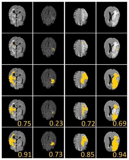
Figure 8.
Brain Tumor Segmentation (using BRATS dataset [28]). Several results from our method using labeled data on the BRATS dataset [28]. The tumor is underlined in yellow. First row: center slices of input. Second row: initial conditions for our algorithm. Third row: ground-truth labels. Fourth row: results from the supervised U-Nets learning method introduced by Ronnenberger et al. [27]. Fifth row: results from our proposed method. The scores in the bottom of each results denote Dice score.
We also compare with the U-net algorithm ([27], see also [31]), tables show the evaluation results, please note that we have suppressed the best and worst 10% of the results, and that for our proposed approach, we have considered only 2 to 4 points as geometric conditions (the initial guess -curve- is automatically constructed from these points), all that leads to make the global results quite homogeneous. We also compare with the Chan-Vese algorithm [11]: in this case, the initial condition is a closed contour located inside the region of interest.
If we use 100% of the BraTS dataset, we obtain the Table 2.
Table 2.
Accuracies of segmentations models on a third of labeled data from BraTS Dataset [28]. We use a Nvidia GeForce RTX 2080 Ti 11G Turbo Edition (Boost frequence: 1545 MHz, GPU memory: 11 GB).
We see that the GPU time is clearly better with our algorithm (and the Chan-Vese one too). The quality is globally equivalent: a little better with our algorithm when not considering the entire database, and equivalent if not. This is an important point because it validates our algorithm when we compare with MR scans segmented with deep learning algorithms with few labeled data.
3.3. Applications to Medical Imaging
Here, we apply our method to 2D medical images, the goal being to outline the cross-sectional area of a great thoracic vessel, namely the main pulmonary artery, in order to non-invasively assess pulmonary arterial hypertension. Figure 9 refers to a slice set perpendicularly to the MPA axis (arrow) of a 78 years old patient, who was suspected of pulmonary arterial hypertension, suffering from breathlessness. The presented magnitude image was acquired from a velocity encoded sequence (Venc = 1.5 m/s), during a 5 min time duration, with a 30 ms temporal resolution (1T Magnetom Expert imager; Siemens; Germany). The image quality is moderate, and in particular the vessel wall is irregular around the arrow, that is, not anatomically possible, and therefore an interpolation in the outlining by the physician is needed.
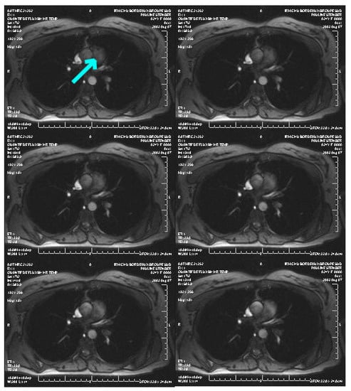
Figure 9.
Example of an image sequence (courtesy of CHU Bordeaux, France). The arrow shows the pulmonary artery to segment.
Since the lack of annotated data is one of the most common limitations encountered in many deep learning approaches like the ones we will study in this subsection, deep leaning approaches are not suitable (at least for now!) for our considered applications.
An example of the segmentation of a pulmonary artery with a curve to interpolate is given in Figure 10. A part of this artery is difficult to segment since its bottom left is always located in a blurred zone.
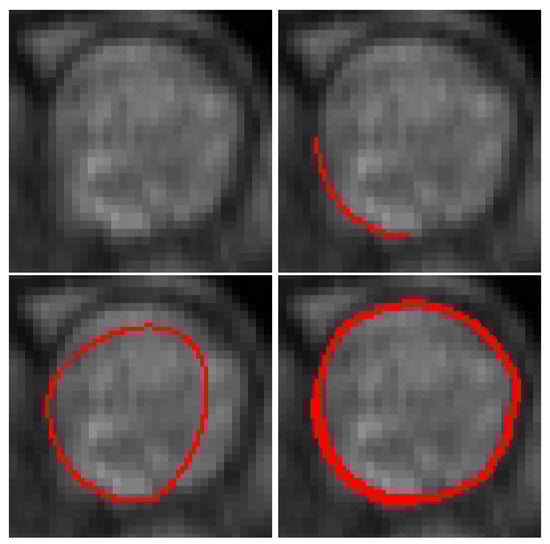
Figure 10.
Blood vessel image, user-defined constraint (top right), initial contour (bottom left) and final (bottom right) contours. Let us note that we have successfully segmented the complete image sequence.
Let us note that the MPA CSA variations versus time, throughout a cardiac cycle, obtained from the present automatic segmentation method are in agreement with previous results obtained from a manual outlining (Hôpital of Bordeaux, France). Moreover, the present method enables us to get a reliable assessment of the systolic-diastolic difference in the vessel CSA, which should lead to a further improvement in the accuracy of a non-invasive blood pressure estimation (using well-known methods, see [32,33]). In several medical applications, let us note that a registration process must be added to the segmentation process (see [34,35,36,37] for more details).
3.4. Applications to Geophysical Imaging
We now apply our algorithm to the segmentation of a non-continuous layer on a geophysical dataset (Figure 11 (right)) extracted from a 3D dataset (Figure 11 (left)). This is a complicated image to segment since there is a vertical fault (see Figure 12). As a priori condition, we here consider a set of point to interpolate (instead of a curve) in order to help the segmentation process (Figure 12). The algorithm starts with a polygonal line interpolating the set of points (to interpolate) as an initial condition, and then segment the image until the edge(s) of the image. Here, the final contour is a segment and not a closed curve, this is of great interest when one wants to track faults or cracks in segmentation processes.
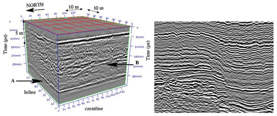
Figure 11.
Left: 3D seismic dataset (courtesy of TotalEnergies, Pau, France). Two strong and continuous reflectors (Horizon A and Horizon B) appear. Right: 2D image (extracted from the 3D seismic dataset) with vertical faults and layers. Considering the complexity of such dataset, it is impossible to segment it without a priori given conditions. The segmentation process consists in finding layers and/or faults.
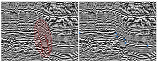
Figure 12.
Left: The red zone underlines the vertical fault (with dotted segments). Right: As a geometric conditions, we consider a set of points given by the user.
The obtained result (Figure 13) has been validated by geophysicians, but the next step requires an algorithm for 3D applications in order to segment 3D geophysical datasets. We are also in the process of creating a free labeled geophysical dataset, in order to test deep learning techniques on these images.
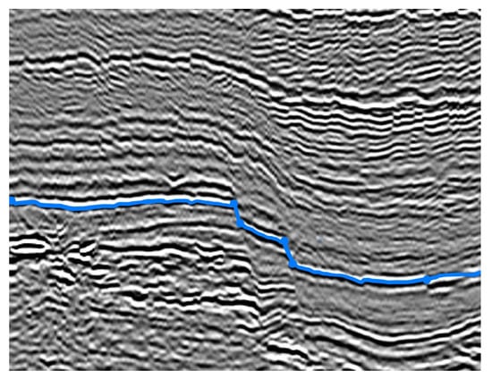
Figure 13.
Final result: we can see that the searched layer is correctly segmented. On this specific dataset, the final contour has to reach the edge of the image: the contour goes beyond the last point to interpolate (right side) to join the edge of the image.
4. Conclusions
We have proposed a method to segment medical or geophysical images with a priori conditions. The efficiency of the method has been shown on 2D images, knowing that such images are difficult to segment with usual approaches since the searched contour is not continuous (geophysical dataset) or when the zone to segment is blurred (medical images).
Compared to Gout et al. [19], the added value brought by our proposed method (automatic initial guess) is materialized by a total number of iterations reduced by a factor of 4 to 60.
The GPU time is also a key point to underline about our algorithm, much lower than deep learning based approaches. About the sensitivity of the model, especially for geophysical data, it is not possible to segment correctly without a precise choice of the interpolation conditions: the choice of such condition strongly impacts the final result, this point is less obvious in medical applications where the choice of the initial condition improves the result only on very noisy areas and/or with a blurred edge, otherwise, the result (whatever the initial condition) is very close to classic algorithms (Chan Vese algorithm for example). The implementation of a 3D code is a work in progress, the main problem for a 3D segmentation process consists in choosing the initial (geometric) condition (a surface, a curve and/or points), which is a complicated task on complex 3D images (mainly because there are 3D data visualization difficulties “to see inside” the 3D dataset, especially in geophysics to give the initial condition—see Figure 14)—the mathematical results remain valid in 3D.
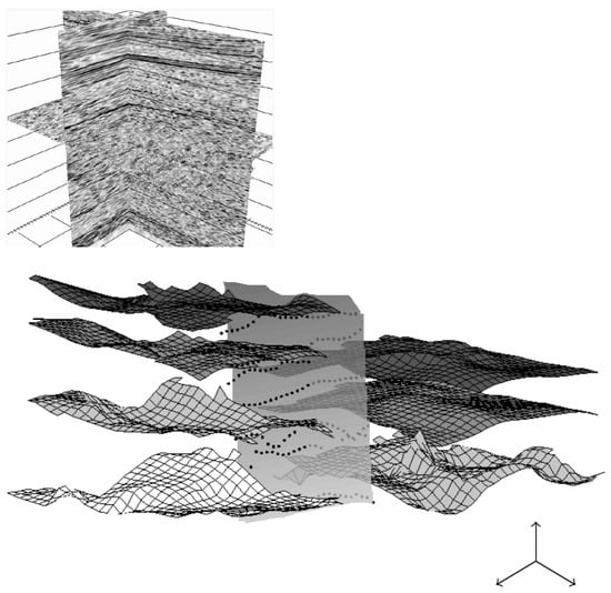
Figure 14.
Top: Another 3D view of the 3D geological dataset of Figure 5. Bottom: From the 3D dataset, we use a set of points (well data given by geologists), and each surface/layer is then constructed with a -spline operator (see [22] for more details on -spline surface approximation). We here automatically construct 7 surfaces that will be considered as an initial condition. Next step consists in the 3D segmentation process from these initial conditions—this last part is a work in progress.
Author Contributions
Conceptualization, G.K., C.G., T.C.-F. and S.K.; methodology, G.K., C.G. and T.C.-F.; software, G.K. and T.C.-F.; validation, G.K., C.G. and S.K.; formal analysis, G.K.; investigation, G.K., C.G., T.C.-F. and S.K.; writing—original draft preparation, G.K.; writing—review and editing, G.K., C.G., T.C.-F. and S.K.; funding acquisition, C.G. All authors have read and agreed to the published version of the manuscript.
Funding
The research was funded by the European Union with the European regional development fund (ERDF, 18P03390/18E01750/18P02733/21E05300) and by the Région Normandie Council via the M2SINUM and DEFHY3GEO projects, Agence Nationale de la Recherche via MEDISEG project (ANR-21-CE23-0013), and Maison Normande des Sciences du Numérique (MNSN, under DSG2-2021 project).
Acknowledgments
The authors thank the CRIANN (Centre Régional Informatique et d’Applications Numériques de Normandie, France) for providing computational resources.
Conflicts of Interest
The authors declare no conflict of interest.
References
- Fukushima, K. Neocognitron: A self-organizing neural network model for a mechanism of pattern recognition unaffected by shift in position. Biol. Cybern. 1980, 36, 193–202. [Google Scholar] [CrossRef] [PubMed]
- Waibel, A.; Hanazawa, T.; Hinton, G.; Shikano, K.; Lang, K.J. Phoneme recognition using time-delay neural networks. IEEE Trans. Acoust. Speech Signal Process. 1989, 37, 328–339. [Google Scholar] [CrossRef]
- LeCun, Y.; Bottou, L.; Bengio, Y.; Haffner, P. Gradient-based learning applied to document recognition. Proc. IEEE 1998, 86, 2278–2324. [Google Scholar] [CrossRef] [Green Version]
- Hochreiter, S.; Schmidhuber, J. Long short-term memory. Neural Comput. 1997, 9, 1735–1780. [Google Scholar] [CrossRef]
- Badrinarayanan, V.; Kendall, A.; Cipolla, R. Segnet: A deep convolutional encoder-decoder architecture for image segmentation. IEEE Trans. Pattern Anal. Mach. Intell. 2017, 39, 2481–2495. [Google Scholar] [CrossRef]
- Goodfellow, I.; Pouget-Abadie, J.; Mirza, M.; Xu, B.; Warde-Farley, D.; Ozair, S.; Courville, A.; Bengio, Y. Generative adversarial nets. In Proceedings of the Advances in Neural Information Processing Systems 27: Annual Conference on Neural Information Processing Systems 2014, Montreal, QC, Canada, 8–13 December 2014; pp. 2672–2680. [Google Scholar]
- Minaee, S.; Boykov, Y.Y.; Porikli, F.; Plaza, A.J.; Kehtarnavaz, N.; Terzopoulos, D. Image Segmentation Using Deep Learning: A Survey. IEEE Trans. Pattern Anal. Mach. Intell. 2021, 1. [Google Scholar] [CrossRef]
- Fantazzini, A.; Esposito, M.; Finotello, A.; Auricchio, F.; Conti, M.; Pane, B.; Spinella, G. 3D Automatic Segmentation of Aortic Computed Tomography Angiography Combining Multi-View 2D Convolutional Neural Networks. Cardiovasc. Eng. Tech. 2020, 11, 576–586. [Google Scholar] [CrossRef]
- Luo, Q.; Wang, L.; Lv, J.; Xiang, S.; Pan, C. Few-shot learning via feature hallucination with variational inference. In Proceedings of the IEEE Winter Conference on Applications of Computer Vision (WACV), Waikoloa, HI, USA, 3–8 January 2021; pp. 3963–3972. [Google Scholar]
- Kass, M.; Witkin, A.; Terzopoulos, D. Snakes: Active contour models. Int. J. Comput. Vis. 1988, 1, 321–331. [Google Scholar] [CrossRef]
- Chan, T.F.; Vese, L.A. Active contours without edges. IEEE Trans. Image Process. 2001, 10, 266–277. [Google Scholar] [CrossRef] [Green Version]
- Mumford, D.; Shah, J. Optimal approximation by piecewise smooth functions and associated variational problems. Comm. Pure Appl. Math. 1989, 42, 577–685. [Google Scholar] [CrossRef] [Green Version]
- Vese, L.; Le Guyader, C. Variational Methods in Image Processing; CRC Press: Boca Raton, FL, USA; Taylor and Francis: Oxfordshire, UK, 2015; 410p, ISBN 9781439849736. [Google Scholar]
- Sethian, J.A. A fast marching level set method for monotonically advancing fronts. Proc. Natl. Acad. Sci. USA 1996, 93, 1591–1595. [Google Scholar] [CrossRef] [PubMed] [Green Version]
- Forcadel, N.; Le Guyader, C.; Gout, C. Generalized fast marching method: Applications to image segmentation. Numer. Algorithms 2008, 48, 189–211. [Google Scholar] [CrossRef]
- Caselles, V.; Kimmel, R.; Sapiro, G. Geodesic Active Contours. Int. J. Comput. Vis. 1997, 22, 61–79. [Google Scholar] [CrossRef]
- Le Guyader, C.; Lambert, Z.; Petitjean, C. Analysis of the weighted Van der Waals-Cahn-Hilliard model for image segmentation. In Proceedings of the 10th International Conference on Image Processing Theory, Tools and Applications IPTA 2020, Paris, France, 9–12 November 2020. [Google Scholar]
- Cremers, D.; Sochen, N.; Schnörr, C. Towards Recognition-Based Variational Segmentation Using Shape Priors and Dynamic Labeling. Lect. Notes Comput. Sci. 2003, 2695, 388–400. [Google Scholar]
- Gout, C.; Le Guyader, C.; Vese, L. Segmentation under geometrical conditions using geodesic active contours and interpolation using level set methods. Numer. Algorithms 2005, 39, 155–173. [Google Scholar] [CrossRef] [Green Version]
- Gout, C.; Le Guyader, C. Geodesic active contour under geometrical conditions: Theory and 3D applications. Numer. Algorithms 2008, 48, 105–133. [Google Scholar]
- Gout, C.; Vieira-Teste, S. Using deformable models to segment complex structures under geometric constraints. In Proceedings of the 4th IEEE Southwest Symposium on Image Analysis and Interpretation, Austin, TX, USA, 2–4 April 2000; pp. 101–105. [Google Scholar]
- Gout, C.; Lambert, Z.; Apprato, D. Data Approximation: Mathematical Modelling and Numerical Simulations; INSA Rouen Normandie; EDP Sciences: Les Ulis, France, 2019; 168p, ISBN 9978-2-7598-2367-3. [Google Scholar]
- Osher, S.; Sethian, J.A. Fronts propagating with curvature dependent speed: Algorithms based on Hamilton-Jacobi formulations. J. Comput. Phys. 1988, 79, 12–49. [Google Scholar] [CrossRef] [Green Version]
- Osher, S.; Fedkiw, R. Level Set Methods and Dynamic Implicit Surfaces; Springer: Cham, Switzerland, 2003. [Google Scholar]
- Weickert, J.; Kühne, G. Fast methods for implicit active contours models. In Geometric Level Set Methods in Imaging, Vision, and Graphics; Springer: New York, NY, USA, 2003. [Google Scholar]
- Cohen, L.D. On active contours models and balloons. Comput. Vision Graph. Image Process. Image Underst. 1991, 53, 211–218. [Google Scholar] [CrossRef]
- Ronneberger, O.; Fischer, P.; Brox, T. U-net: Convolutional networks for biomedical image segmentation. In Proceedings of the MICCAI International Conference on Medical Image Computing and Computer-Assisted Intervention, Munich, Germany, 5–9 October 2015; Springer: Cham, Switzerland, 2015; pp. 234–241. [Google Scholar]
- Menze, B.H.; Jakab, A.; Bauer, S.; Kalpathy-Cramer, J.; Farahani, K.; Kirby, J.; Burren, Y.; Porz, N.; Slotboom, J.; Wiest, R.; et al. The multimodal brain tumor image segmentation benchmark (BRATS). IEEE Trans. Med. Imaging 2014, 34, 1993–2024. [Google Scholar] [CrossRef]
- Kingma, D.P.; Ba, J. Adam: A method for stochastic optimization, International Conference on Learning Representations. arXiv 2015, arXiv:1412.6980. [Google Scholar]
- Jaccard, P. Distribution de la flore alpine dans le bassin des Dranses et dans quelques régions voisines. Bull. SociéTé Vaudoise Sci. Nat. 1901, 37, 241–272. [Google Scholar]
- Kim, B.; Ye, J.C. Cycle-Consistent Adversarial Network with Polyphase U-Nets for Liver Lesion Segmentation. 2018. Available online: https://openreview.net/pdf?id=SyQtAooiz (accessed on 2 March 2021).
- Laffon, E.; Laurent, F.; Bernard, V.; De Boucaud, L.; Ducassou, D.; Marthan, R. Noninvasive assessment of pulmonary arterial hypertension by MR phase-mapping method. J. Appl. Physiol. 2001, 90, 2197–2202. [Google Scholar] [CrossRef] [PubMed] [Green Version]
- Laffon, E.; Vallet, C.; Bernard, V.; Montaudon, M.; Ducassou, D.; Laurent, F.; Marthan, R. A computed method for non invasive MRI assessment of pulmonary arterial hypertension. J. Appl. Physiol. 2004, 96, 463–468. [Google Scholar] [CrossRef]
- Debroux, N.; Le Guyader, C. A joint segmentation/registration model based on a nonlocal characterization of weighted total variation and nonlocal shape descriptors. SIAM J. Imaging Sci. 2018, 11, 957–990. [Google Scholar] [CrossRef]
- Ozeré, S.; Le Guyader, C.; Gout, C. Joint segmentation/registration model by shape alignment via weighted total variation minimization and nonlinear elasticity. SIAM J. Imaging Sci. 2015, 8, 1981–2020. [Google Scholar] [CrossRef]
- Gout, C.; Le Guyader, C.; Romani, L.; Saint-Guirons, A.-G. Approximation of surfaces with fault(s) and/or rapidly varying data, using a segmentation process, Dm-splines and the finite element method. Numer. Algorithms 2008, 48, 67–92. [Google Scholar] [CrossRef]
- Le Guyader, C.; Apprato, D.; Gout, C. On the Construction of Topology-Preserving Deformation Fields. IEEE Trans. Image Process. 2012, 21, 1587–1599. [Google Scholar] [CrossRef] [PubMed]
Publisher’s Note: MDPI stays neutral with regard to jurisdictional claims in published maps and institutional affiliations. |
© 2022 by the authors. Licensee MDPI, Basel, Switzerland. This article is an open access article distributed under the terms and conditions of the Creative Commons Attribution (CC BY) license (https://creativecommons.org/licenses/by/4.0/).