In Vivo Validation of a Cardiovascular Simulation Model in Pigs

 , , ,
, , ,
Abstract
1. Introduction
2. Materials and Methods
2.1. Animal Model
2.1.1. Induction and Maintenance of Anaesthesia
2.1.2. Surgical Instrumentation
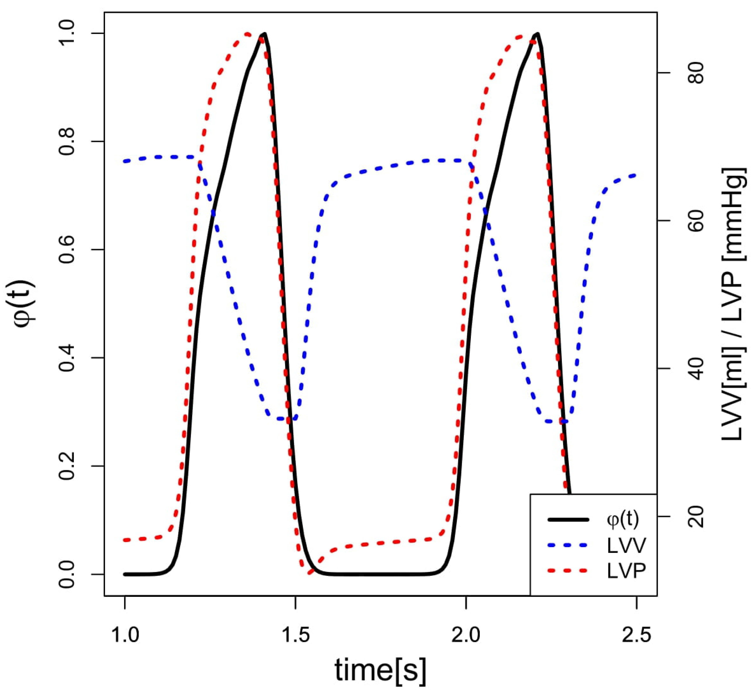
2.2. Data Acquisition and Calculations
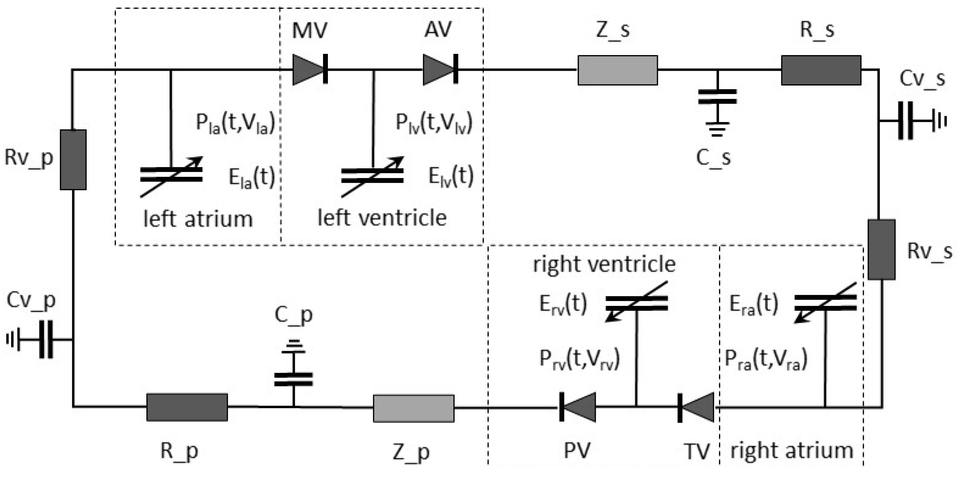
2.3. Simulation Model
2.4. Statistics
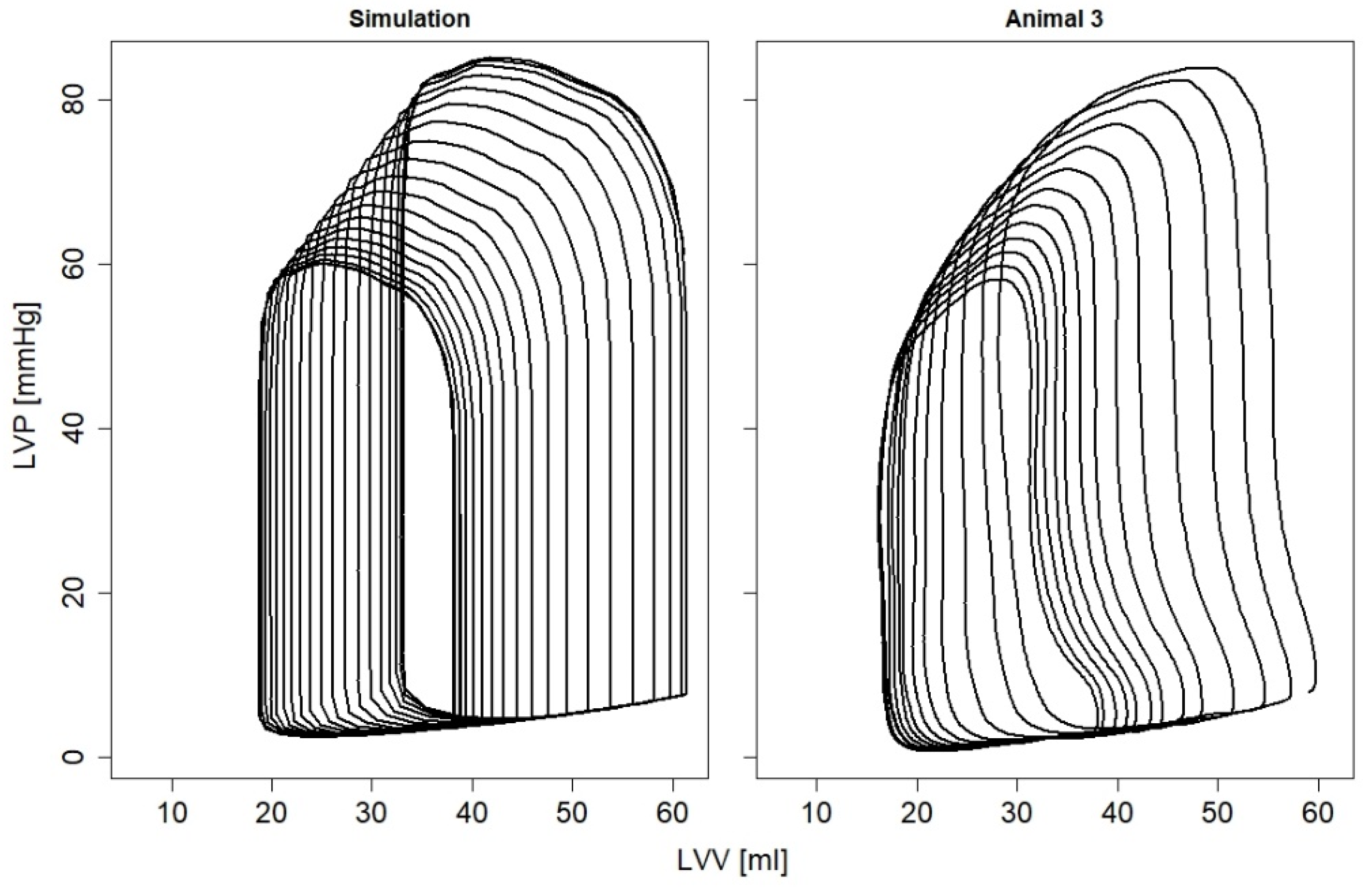
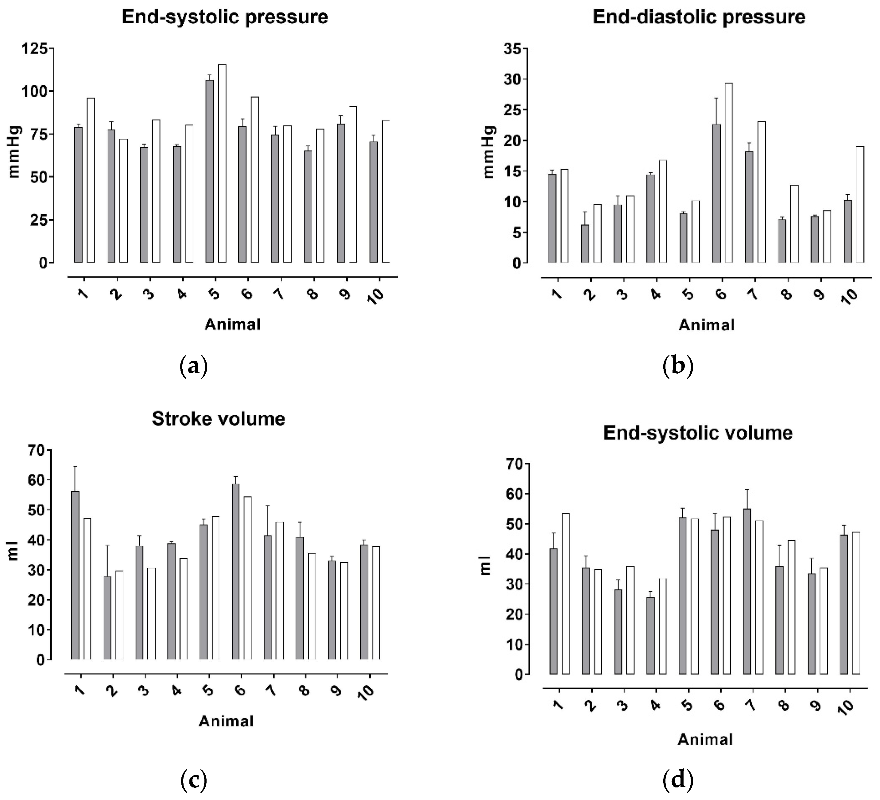
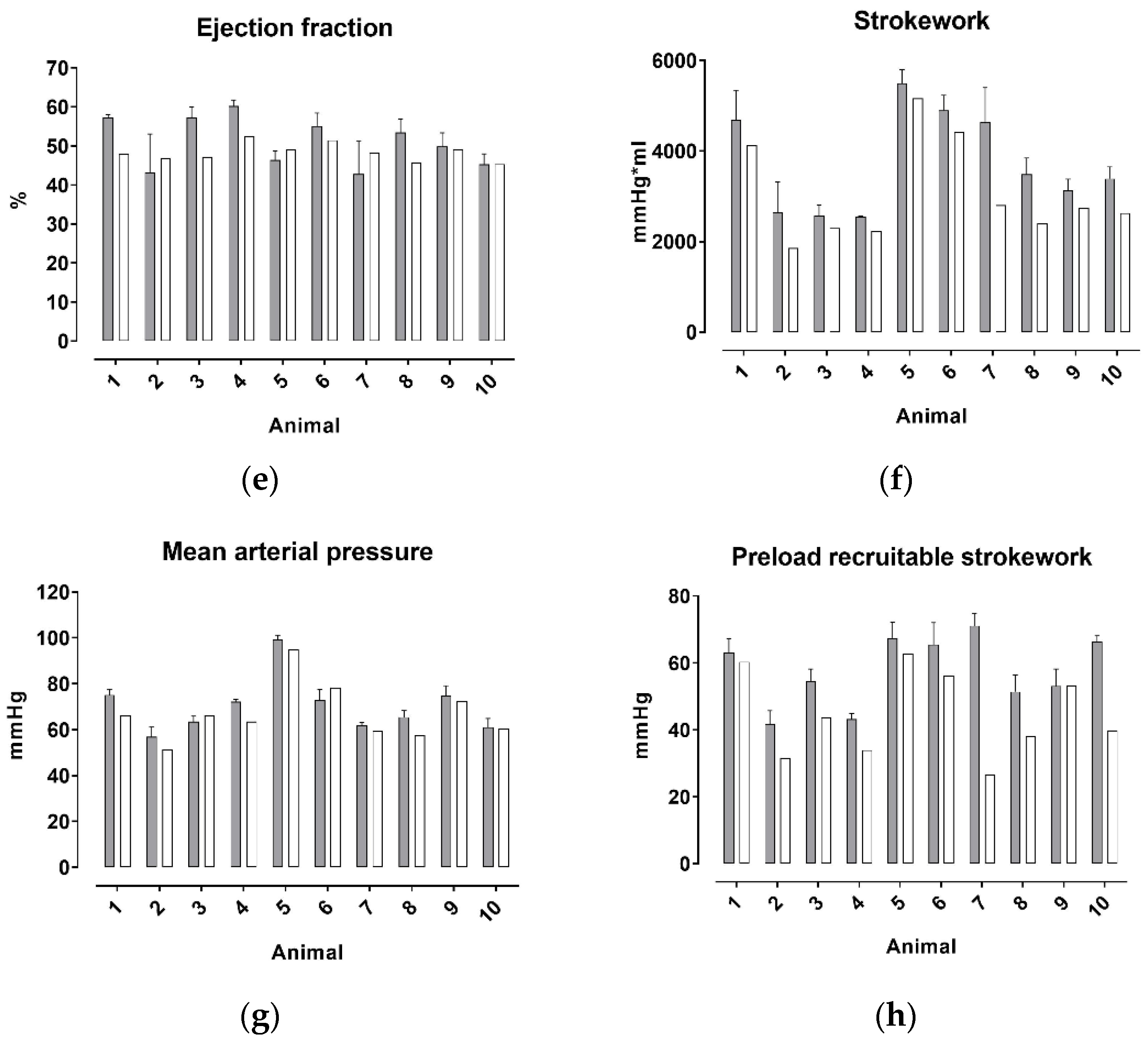
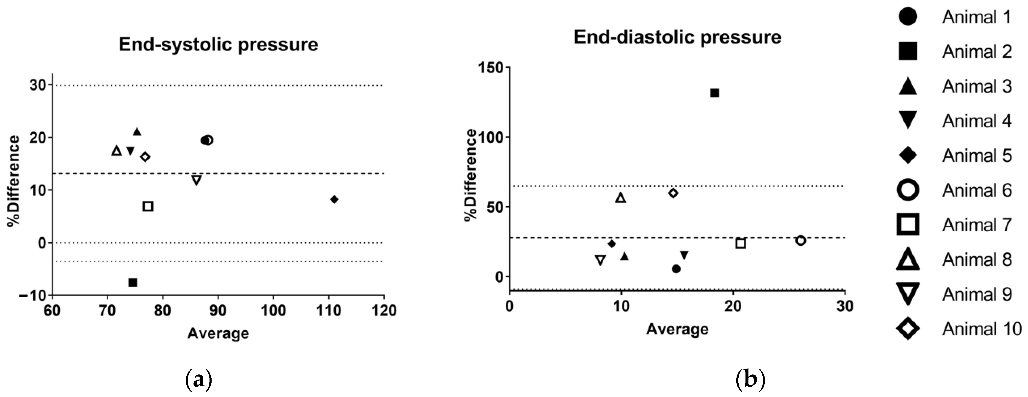
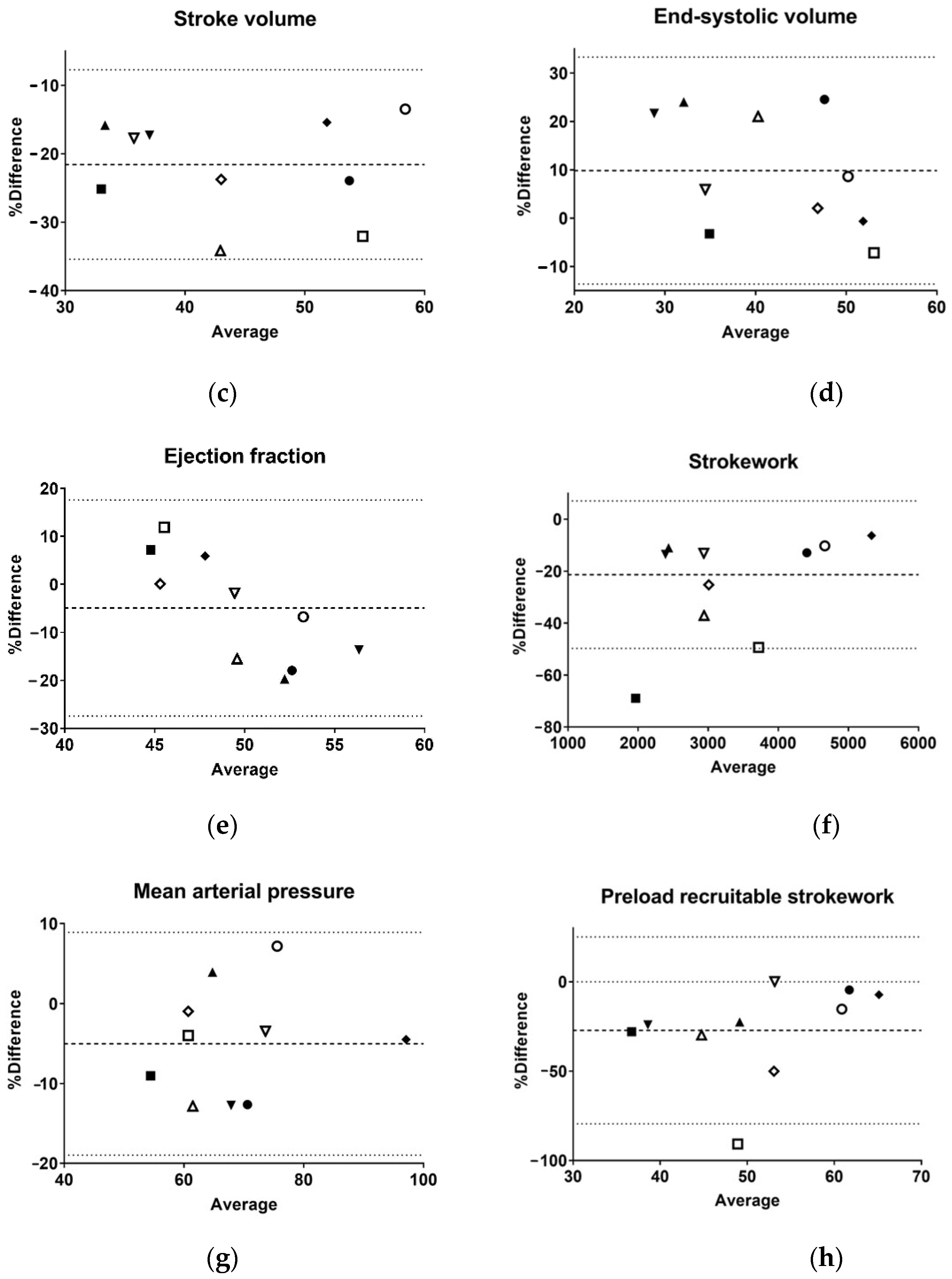
3. Results
4. Discussion
5. Conclusions
Supplementary Materials
Author Contributions
Funding
Institutional Review Board Statement
Data Availability Statement
Conflicts of Interest
References
- Scardulla, F.; Pasta, S.; D’Acquisto, L.; Sciacca, S.; Agnese, V.; Vergara, C.; Quarteroni, A.; Clemenza, F.; Bellavia, D.; Pilato, M. Shear stress alterations in the celiac trunk of patients with a continuous-flow left ventricular assist device as shown by in-silico and in-vitro flow analyses. J. Heart Lung Transplant. 2017, 36, 906–913. [Google Scholar] [CrossRef] [PubMed]
- Scardulla, F.; Bellavia, D.; D’Acquisto, L.; Raffa, G.M.; Pasta, S. Particle image velocimetry study of the celiac trunk hemodynamic induced by continuous-flow left ventricular assist device. Med. Eng. Phys. 2017, 47, 47–54. [Google Scholar] [CrossRef]
- Habigt, M.; Ketelhut, M.; Gesenhues, J.; Schrodel, F.; Hein, M.; Mechelinck, M.; Schmitz-Rode, T.; Abel, D.; Rossaint, R. Comparison of novel physiological load-adaptive control strategies for ventricular assist devices. Biomed. Tech. Berl. 2017, 62, 149–160. [Google Scholar] [CrossRef] [PubMed]
- Noordergraaf, A.; Verdouw, P.D.; Boom, H.B. The use of an analog computer in a circulation model. Prog. Cardiovasc. Dis. 1963, 5, 419–439. [Google Scholar] [CrossRef]
- Guyton, A.C.; Coleman, T.G.; Granger, H.J. Circulation: Overall regulation. Annu. Rev. Physiol. 1972, 34, 13–44. [Google Scholar] [CrossRef] [PubMed]
- Suga, H.; Sagawa, K.; Shoukas, A.A. Load independence of the instantaneous pressure-volume ratio of the canine left ventricle and effects of epinephrine and heart rate on the ratio. Circ. Res. 1973, 32, 314–322. [Google Scholar] [CrossRef]
- Leaning, M.; Pullen, H.E.; Carson, E.R.; Finkelstein, L. Modelling a complex biological system: The human cardiovascular system—1. Methodology and model description. Trans. Inst. Meas. Control. 1983, 5, 71–86. [Google Scholar] [CrossRef]
- Ursino, M. Interaction between carotid baroregulation and the pulsating heart: A mathematical model. Am. J. Physiol. 1998, 275, H1733–H1747. [Google Scholar] [CrossRef]
- Segers, P.; Stergiopulos, N.; Schreuder, J.J.; Westerhof, B.E.; Westerhof, N. Left ventricular wall stress normalization in chronic pressure-overloaded heart: A mathematical model study. Am. J. Physiol. Heart Circ. Physiol. 2000, 279, H1120–H1127. [Google Scholar] [CrossRef]
- Vollkron, M.; Schima, H.; Huber, L.; Wieselthaler, G. Interaction of the Cardiovascular System with an Implanted Rotary Assist Device: Simulation Study with a Refined Computer Model. Artif. Organs 2002, 26, 349–359. [Google Scholar] [CrossRef]
- Smith, B.W.; Chase, J.G.; Nokes, R.I.; Shaw, G.M.; Wake, G. Minimal haemodynamic system model including ventricular interaction and valve dynamics. Med. Eng. Phys. 2004, 26, 131–139. [Google Scholar] [CrossRef] [PubMed]
- Colacino, F.M.; Moscato, F.; Piedimonte, F.; Arabia, M.; Danieli, G.A. Left ventricle load impedance control by apical VAD can help heart recovery and patient perfusion: A numerical study. ASAIO J. 2007, 53, 263–277. [Google Scholar] [CrossRef] [PubMed]
- Welp, C.; Werner, J.; Böhringer, D.; Hexamer, M. Investigation of cardiac and cardio-therapeutical phenomena using a pulsatile circulatory model. Biomed. Tech. 2004, 49, 327–331. [Google Scholar] [CrossRef]
- Arts, T.; Delhaas, T.; Bovendeerd, P.; Verbeek, X.; Prinzen, F.W. Adaptation to mechanical load determines shape and properties of heart and circulation: The CircAdapt model. Am. J. Physiol. Heart Circ. Physiol. 2005, 288, H1943–H1954. [Google Scholar] [CrossRef]
- Bovendeerd, P.H.; Borsje, P.; Arts, T.; van De Vosse, F.N. Dependence of intramyocardial pressure and coronary flow on ventricular loading and contractility: A model study. Ann. Biomed. Eng. 2006, 34, 1833–1845. [Google Scholar] [CrossRef]
- Ottesen, J.T.; Danielsen, M. Modeling ventricular contraction with heart rate changes. J. Theor. Biol. 2003, 222, 337–346. [Google Scholar] [CrossRef]
- Gesenhues, J.; Hein, M.; Albin, T.; Rossaint, R.; Abel, D. Cardiac Modeling: Identification of Subject Specific Left-Ventricular Isovolumic Pressure Curves. IFAC-PapersOnLine 2015, 48, 581–586. [Google Scholar] [CrossRef]
- Westerhof, N.; Elzinga, G.; Sipkema, P. An artificial arterial system for pumping hearts. J. Appl. Physiol. 1971, 31, 776–781. [Google Scholar] [CrossRef]
- Burattini, R.; Knowlen, G.G.; Campbell, K.B. Two arterial effective reflecting sites may appear as one to the heart. Circ. Res. 1991, 68, 85–99. [Google Scholar] [CrossRef]
- O’Rourke, M.F. Pressure and flow waves in systemic arteries and the anatomical design of the arterial system. J. Appl. Physiol. 1967, 23, 139–149. [Google Scholar] [CrossRef]
- Wetterer, E.; Kenner, T. Grundlagen der Dynamik des Arterienpulses; Springer: Berlin/Heidelberg, Germany, 1968. [Google Scholar]
- O’Rourke, M.F.; Avolio, A.P. Pulsatile flow and pressure in human systemic arteries. Studies in man and in a multibranched model of the human systemic arterial tree. Circ. Res. 1980, 46, 363–372. [Google Scholar] [CrossRef] [PubMed]
- Stergiopulos, N.; Young, D.F.; Rogge, T.R. Computer simulation of arterial flow with applications to arterial and aortic stenoses. J. Biomech. 1992, 25, 1477–1488. [Google Scholar] [CrossRef]
- Westerhof, N.; Bosman, F.; De Vries, C.J.; Noordergraaf, A. Analog studies of the human systemic arterial tree. J. Biomech. 1969, 2, 121–143. [Google Scholar] [CrossRef]
- Avolio, A.P. Multi-branched model of the human arterial system. Med. Biol. Eng. Comput. 1980, 18, 709–718. [Google Scholar] [CrossRef] [PubMed]
- Lu, K.; Clark, J.W., Jr.; Ghorbel, F.H.; Ware, D.L.; Bidani, A. A human cardiopulmonary system model applied to the analysis of the Valsalva maneuver. Am. J. Physiol. Heart Circ. Physiol. 2001, 281, H2661–H2679. [Google Scholar] [CrossRef] [PubMed]
- Gesenhues, J.; Hein, M.; Habigt, M.; Mechelinck, M.; Albin, T.; Abel, D. Nonlinear object-oriented modeling based optimal control of the heart: Performing precise preload manipulation maneuvers using a ventricular assist device. In Proceedings of the 2016 European Control Conference (ECC), Aalborg, Denmark, 29 June–1 July 2016; pp. 2108–2114. [Google Scholar]
- National Research Council Committee for the Update of the Guide for the Care and Use of Laboratory Animals. The National Academies Collection: Reports Funded by National Institutes of Health. In Guide for the Care and Use of Laboratory Animals; National Academies Press, National Academy of Sciences: Washington, DC, USA, 2011. [Google Scholar]
- Pierce, E. Wikipedia, File:Heart normal.svg. Available online: https://en.wikipedia.org/wiki/File:Heart_normal.svg (accessed on 16 March 2022).
- Baan, J.; Van Der Velde, E.T.; De Bruin, H.G.; Smeenk, G.J.; Koops, J.; Van Dijk, A.D.; Temmerman, D.; Senden, J.; Buis, B. Continuous measurement of left ventricular volume in animals and humans by conductance catheter. Circulation 1984, 70, 812–823. [Google Scholar] [CrossRef]
- De Vroomen, M.; Cardozo, R.H.L.; Steendijk, P.; van Bel, F.; Baan, J. Improved contractile performance of right ventricle in response to increased RV afterload in newborn lamb. Am. J. Physiol. Heart Circ. Physiol. 2000, 278, H100–H105. [Google Scholar] [CrossRef]
- Steendijk, P.; Baan, J. Comparison of intravenous and pulmonary artery injections of hypertonic saline for the assessment of conductance catheter parallel conductance. Cardiovasc. Res. 2000, 46, 82–89. [Google Scholar] [CrossRef]
- Liu, Z.; Brin, K.P.; Yin, F.C. Estimation of total arterial compliance: An improved method and evaluation of current methods. Am. J. Physiol. 1986, 251 Pt 2, H588–H600. [Google Scholar] [CrossRef]
- Brimioulle, S.; Maggiorini, M.; Stephanazzi, J.; Vermeulen, F.; Lejeune, P.; Naeije, R. Effects of low flow on pulmonary vascular flow-pressure curves and pulmonary vascular impedance. Cardiovasc. Res. 1999, 42, 183–192. [Google Scholar] [CrossRef]
- Chung, D.C.; Niranjan, S.C.; Clark, J.W., Jr.; Bidani, A.; Johnston, W.E.; Zwischenberger, J.B.; Traber, D.L. A dynamic model of ventricular interaction and pericardial influence. Am. J. Physiol. 1997, 272 Pt 2, H2942–H2962. [Google Scholar] [PubMed]
- Hein, M.; Roehl, A.B.; Baumert, J.H.; Bleilevens, C.; Fischer, S.; Steendijk, P.; Rossaint, R. Xenon and isoflurane improved biventricular function during right ventricular ischemia and reperfusion. Acta Anaesthesiol. Scand. 2010, 54, 470–478. [Google Scholar] [CrossRef] [PubMed]
- Gesenhues, J.; Hein, M.; Ketelhut, M.; Habigt, M.; Rüschen, D.; Mechelinck, M.; Albin, T.; Leonhardt, S.; Schmitz-Rode, T.; Rossaint, R.; et al. Benefits of object-oriented models and ModeliChart: Modern tools and methods for the interdisciplinary research on smart biomedical technology. Biomed. Tech. 2017, 62, 111–121. [Google Scholar] [CrossRef]
- Segers, P.; Verdonck, P.; Deryck, Y.; Brimioulle, S.; Naeije, R.; Carlier, S.; Stergiopulos, N. Pulse pressure method and the area method for the estimation of total arterial compliance in dogs: Sensitivity to wave reflection intensity. Ann. Biomed. Eng. 1999, 27, 480–485. [Google Scholar] [CrossRef] [PubMed]
- Stergiopulos, N.; Meister, J.J.; Westerhof, N. Simple and accurate way for estimating total and segmental arterial compliance: The pulse pressure method. Ann. Biomed. Eng. 1994, 22, 392–397. [Google Scholar] [CrossRef] [PubMed]
- Gesenhues, J.; Hein, M.; Ketelhut, M.; Albin, T.; Abel, D. Towards Medical Cyber-Physical Systems: Modelica and FMI based Online Parameter Identification of the Cardiovascular System. In Proceedings of the 12th International Modelica Conference, Prague, Czech Republic, 15–17 May 2017; Linköping University Electronic Press: Linköping, Sweden, 2017; pp. 613–621. [Google Scholar]
- Brimioulle, S.; Wauthy, P.; Ewalenko, P.; Rondelet, B.; Vermeulen, F.; Kerbaul, F.; Naeije, R. Single-beat estimation of right ventricular end-systolic pressure-volume relationship. Am. J. Physiol. Heart Circ. Physiol. 2003, 284, H1625–H1630. [Google Scholar] [CrossRef] [PubMed]
- Freeman, G.L.; Little, W.C.; O’Rourke, R.A. The effect of vasoactive agents on the left ventricular end-systolic pressure-volume relation in closed-chest dogs. Circulation 1986, 74, 1107–1113. [Google Scholar] [CrossRef] [PubMed]
- Little, W.C.; Cheng, C.P.; Mumma, M.; Igarashi, Y.; Vinten-Johansen, J.; Johnston, W.E. Comparison of measures of left ventricular contractile performance derived from pressure-volume loops in conscious dogs. Circulation 1989, 80, 1378–1387. [Google Scholar] [CrossRef] [PubMed]
- Burkhoff, D.; Sugiura, S.; Yue, D.T.; Sagawa, K. Contractility-dependent curvilinearity of end-systolic pressure-volume relations. Am. J. Physiol. 1987, 252, H1218–H1227. [Google Scholar] [CrossRef]
- Kass, D.A.; Beyar, R.; Lankford, E.; Heard, M.; Maughan, W.L.; Sagawa, K. Influence of contractile state on curvilinearity of in situ end-systolic pressure-volume relations. Circulation 1989, 79, 167–178. [Google Scholar] [CrossRef]
- Nordhaug, D.; Steensrud, T.; Korvald, C.; Aghajani, E.; Myrmel, T. Preserved myocardial energetics in acute ischemic left ventricular failure—Studies in an experimental pig model. Eur. J. Cardiothorac. Surg. 2002, 22, 135–142. [Google Scholar] [CrossRef]
- Vandenberghe, S.; Segers, P.; Steendijk, P.; Meyns, B.; Dion, R.A.; Antaki, J.F.; Verdonck, P. Modeling ventricular function during cardiac assist: Does time-varying elastance work? ASAIO J. 2006, 52, 4–8. [Google Scholar] [CrossRef] [PubMed]
- Sack, K.L.; Dabiri, Y.; Franz, T.; Solomon, S.D.; Burkhoff, D.; Guccione, J.M. Investigating the Role of Interventricular Interdependence in Development of Right Heart Dysfunction During LVAD Support: A Patient-Specific Methods-Based Approach. Front. Physiol. 2018, 9, 520. [Google Scholar] [CrossRef] [PubMed]
- Cingolani, H.E.; Perez, N.G.; Cingolani, O.H.; Ennis, I.L. The Anrep effect: 100 years later. Am. J. Physiol. Heart Circ. Physiol. 2013, 304, H175–H182. [Google Scholar] [CrossRef] [PubMed]
- Westerhof, N.; Lankhaar, J.W.; Westerhof, B.E. The arterial Windkessel. Med. Biol. Eng. Comput. 2009, 47, 131–141. [Google Scholar] [CrossRef] [PubMed]


| Input Parameter | Animal | HR | E_ES | V0_ES | λ | P0_ED | V0_ED | Cs | Z0 | Zc | V0_sC (Simulation Only) |
|---|---|---|---|---|---|---|---|---|---|---|---|
| Simulation/Animal | 1 | 101 | 1.33 | −19.02 | 0.0365 | 0.2126 | −19.36 | 1.7298 | 0.7341 | 0.0894 | 1100 |
| 2 | 91 | 1.14 | −28.94 | 0.0478 | 0.0394 | −50.48 | 0.9835 | 1.0017 | 0.1029 | 1865 | |
| 3 | 100 | 1.41 | −23.62 | 0.0263 | 0.3675 | −63.38 | 1.7140 | 1.0959 | 0.1102 | 1700 | |
| 4 | 75 | 1.01 | −48.25 | 0.0253 | 0.7728 | −55.30 | 1.5443 | 1.3407 | 0.0944 | 1680 | |
| 5 | 79 | 1.13 | −51.44 | 0.0236 | 0.2142 | −64.57 | 2.2253 | 1.2959 | 0.0994 | 1382 | |
| 6 | 84 | 1.60 | −8.09 | 0.0254 | 0.3502 | −67.20 | 1.9238 | 0.8044 | 0.0888 | 580 | |
| 7 | 85 | 0.80 | −48.74 | 0.0280 | 0.5369 | −38.80 | 1.7860 | 0.7217 | 0.0840 | 1060 | |
| 8 | 91 | 1.04 | −30.67 | 0.0444 | 0.0110 | −80.21 | 1.7580 | 0.8584 | 0.1142 | 1600 | |
| 9 | 98 | 1.52 | −24.77 | 0.0218 | 0.5375 | −61.07 | 1.4927 | 1.1763 | 0.1074 | 1730 | |
| 10 | 106 | 1.34 | −14.98 | 0.0413 | 0.0053 | −113.60 | 1.2890 | 0.7172 | 0.0951 | 1250 | |
| Mean | 49.2 | 1.23 | −29.85 | 0.0320 | 0.3047 | −61.4 | 1.6446 | 0.9746 | 0.0986 | 1395 | |
| CV [%] | 22.0 | 20.28 | 50.4 | 29.8 | 84.5 | 40.5 | 20.8 | 24.8 | 10.1 | 28.6 |
| P_ES | P_ED | SV | V_ED | V_ES | EF | SW | MAP | PRSW | |
|---|---|---|---|---|---|---|---|---|---|
| BIAS [%] | 13.1 | 28.0 | −21.6 | −0.1 | 9.8 | −4.9 | −21.3 | −5.0 | −27.2 |
| 95% Limits of Agreement | |||||||||
| From | −3.6 | −8.9 | −35.4 | −1.7 | −13.6 | −27.4 | −49.7 | −19.0 | −79.5 |
| To | 29.9 | 64.8 | −7.7 | 1.5 | 33.3 | 17.6 | 7.0 | 8.9 | 25.1 |
| Coefficient of variation | 15.4 | 45.7 | 22.7 | 20.2 | 24.9 | 12.6 | 29.1 | 17.1 | 18.0 |
Publisher’s Note: MDPI stays neutral with regard to jurisdictional claims in published maps and institutional affiliations. |
© 2022 by the authors. Licensee MDPI, Basel, Switzerland. This article is an open access article distributed under the terms and conditions of the Creative Commons Attribution (CC BY) license (https://creativecommons.org/licenses/by/4.0/).
Share and Cite
Habigt, M.A.; Gesenhues, J.; Stemmler, M.; Hein, M.; Rossaint, R.; Mechelinck, M. In Vivo Validation of a Cardiovascular Simulation Model in Pigs. Math. Comput. Appl. 2022, 27, 28. https://doi.org/10.3390/mca27020028
Habigt MA, Gesenhues J, Stemmler M, Hein M, Rossaint R, Mechelinck M. In Vivo Validation of a Cardiovascular Simulation Model in Pigs. Mathematical and Computational Applications. 2022; 27(2):28. https://doi.org/10.3390/mca27020028
Chicago/Turabian StyleHabigt, Moriz A., Jonas Gesenhues, Maike Stemmler, Marc Hein, Rolf Rossaint, and Mare Mechelinck. 2022. "In Vivo Validation of a Cardiovascular Simulation Model in Pigs" Mathematical and Computational Applications 27, no. 2: 28. https://doi.org/10.3390/mca27020028
APA StyleHabigt, M. A., Gesenhues, J., Stemmler, M., Hein, M., Rossaint, R., & Mechelinck, M. (2022). In Vivo Validation of a Cardiovascular Simulation Model in Pigs. Mathematical and Computational Applications, 27(2), 28. https://doi.org/10.3390/mca27020028