Time to Critical Condition in Emergency Services

Abstract

Providing uninterrupted response service is of paramount importance for emergency medical services, regardless of the operating scenario. Thus, reliable estimates of the time to the critical condition, under which there will be no available servers to respond to the next incoming call, become very useful measures of the system’s performance. In this contribution, we develop a key performance indicator by providing an explicit formula for the average time to the shortage condition. Our analytical expression for this average time is a function of the number of parallel servers and the inter-arrival and service times. We assume exponential distributions of times in our analytical expression, but for evaluating the mean first-passage time to the critical condition under more realistic scenarios, we validate our result through exhaustive simulations with lognormal service time distributions. For this task, we have implemented a simulator in R. Our results indicate that our analytical formula is an acceptable approximation under any situation of practical interest.

1. Introduction

The problem of assigning resources to respond to a stochastic demand is a ubiquitous topic in operational research. The trade-off between service quality and operational efficiency is a crucial aspect of the Emergency Medical Services (EMS), where the lives of patients depend on the timeliness of care. Thus, the development of Key Performance Indicators (KPIs) to objectively quantify the performance across the operational, clinical and financial departments is a current demand of an industry that is becoming increasingly data-driven. KPIs are the basic tools for planners, and the nature of each KPI selects a particular feature of the system and determines its data gathering strategy.

Among the most intuitive and used operational KPIs in EMS are the successive times involved in the service cycle: call reception, patient triage, dispatch, ambulance turnout, travel from the base to the emergency site, paramedic care, eventual transfer of the patient to a hospital and return of the ambulance to its base. Response time (the interval between the reception of an emergency call and the arrival of a paramedic at the scene of the event) is a common operational metric of EMS, and it is considered a good indication of the quality offered by the service [1]. One reason for its popularity as a KPI resides in the fact that it is directly quantifiable and easily understood by the public and policy makers. Additionally, the EMS industry has the goal of providing care within eight minutes for cardiac arrest [2] and major trauma [3]. However, there is evidence that exceeding that response time criterion does not affect patient survival after a traumatic impact injury [4,5]. Moreover, solutions that only focus on shortening the response time are cost prohibitive and put the safety of patients, attendant crew and the public at risk [6]. A rational approach to the ambulance business process should simultaneously consider multiple metrics and operational trade-off between administrator-oriented and patient-centered KPIs [7].

One of the most important aspects of emergency medical management is avoiding the oversaturation of the system. Therefore, in this work, we consider the First-Passage Time (FPT) [8] to the critical condition, under which there will be not available servers to respond to the next incoming call. Criticality prediction is of special interest for the quality of the medical service (response time off-target) as well as for the financial management of the service, given that, as we will see, the critical condition strongly depends on the number L of ambulances simultaneously in service and because queueing a call may involve transferring it to another EMS. Any system operating under fixed conditions with a given number of servers and a First-Come First-Served (FCFS) discipline is a discrete one-dimensional stochastic process over the occupation states of servers. Therefore, the first-passage time to the state of oversaturation, in which there are no available servers, is finite. The question is how long is that time. Thus, the mean first-passage time (MFPT) becomes a relevant key performance indicator for the operational condition in EMS.

In urban emergency services logistics, there are two distinct fields: capacity planning and location analysis. Both fields are interrelated in the districting problem or how the region should be partitioned into areas of primary responsibility (districts) [9,10]. Here, MFPT can be applied to an operational subarea or district, preferably intended to be independently served by a subset of ambulances (intradistrict dispatches). In this case, MFPT gives us the average time to request an ambulance from another operational zone to answer the next emergency call when the primary equipment is busy (interdistrict dispatches). MFPT can also be a useful KPI in the decision-making process of emergency departments [11,12], where MFPT provides the average time to a shortage of intensive therapy beds when the FCFS discipline is used after the patient’s triage.

Queueing theory has been widely applied in health care in the last 70 years [13]. Since Larson’s seminal article [9], quite a few queueing models have been developed to incorporate the intrinsic probabilistic nature of urban EMS derived from the Poisson nature of the call arrival process and the variability in service times. Multiple queueing systems have been developed that respond with different emphasis on the KPIs selected in each case. In this contribution, we use a birth–death process to properly analyse the dependence of MFPT on the number of servers and the rest of the system’s operational parameters. The birth–death process is basic to queueing models involving exponential inter-arrival and service time distributions. In the Kendall–Lee notation, we have $M/M/L/FCFS/\infty /\infty$ [8]. Thus, our analytical model is based only on two average times: $T_C$, the mean inter-arrival time, and $T_S$, the mean service time of a single server, that is, the time it takes for an ambulance to complete a trip from the instant a call is assigned until the release of this server. Several analytical results are well known in operational research under that assumption [8].

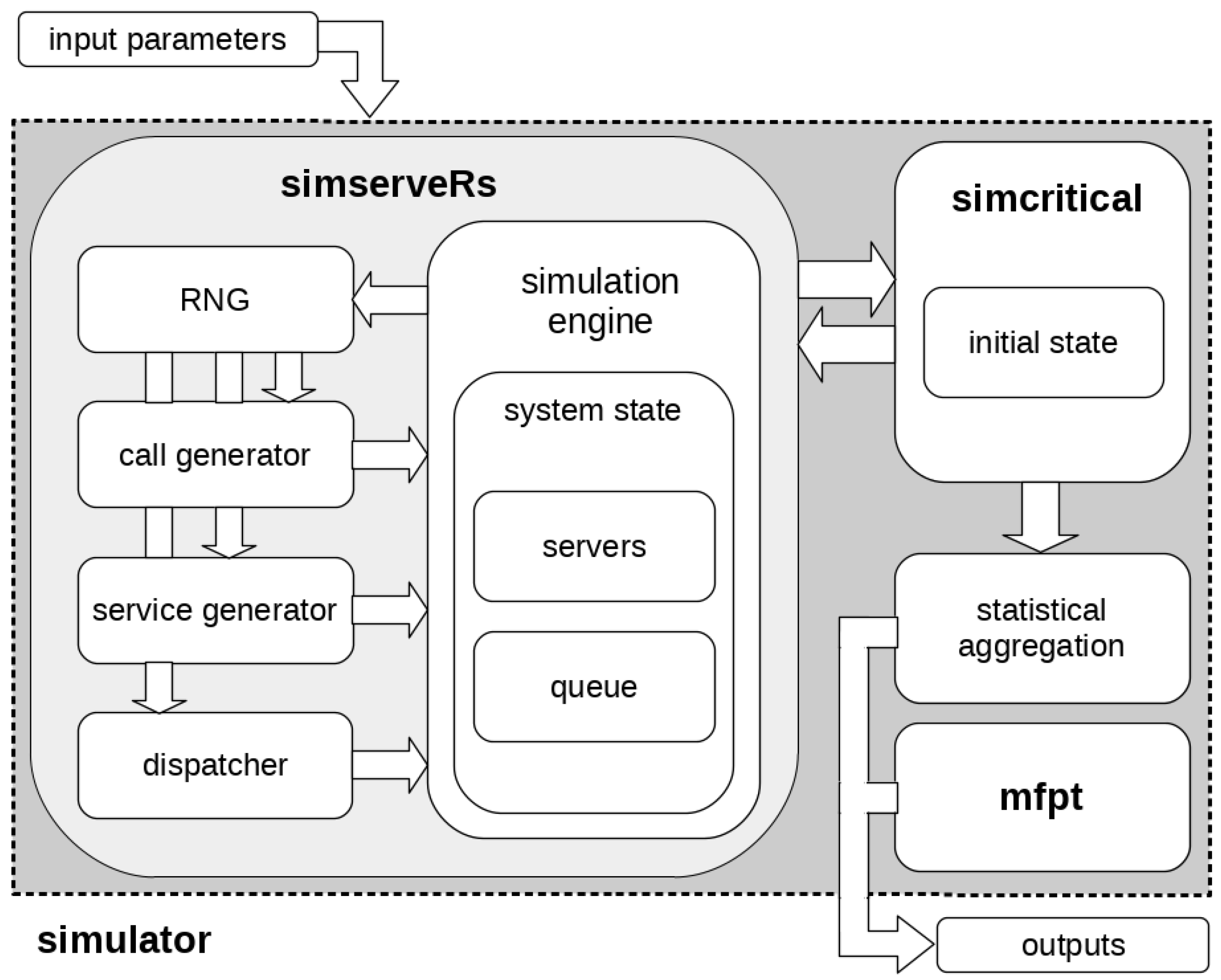
However, experimental evidence from an emergency service indicates that service time distributions are well fitted by lognormal distributions [12,14,15,16]. Hence, our objective is also to numerically evaluate the deviation between analytical and simulated results for MFPT. Thus, we present an R-simulator for a system of L servers in parallel with general distributions for inter-arrival and service times and FCFS discipline: $GI/G/L/FCFS$ [8]. This tool allows the user to calculate the key performance indicators of direct interest in the industry beyond the known analytical results, which are limited to exponential distributions. Particularly, we show our work on Mean First-Passage Time (MFPT) to system critical condition.

In this way, the motivation of our work is two-fold. On the one hand, we provide an explicit analytical expression for the MFPT to the critical condition, and, on the other hand, under more realistic conditions, we analyse the validity of our assumptions through exhaustive simulations. In Section 2, we provide our analytical expression for MFPT and explore the generic nature of the method, postponing detailed mathematical derivations to the appendices. Additionally, in that section, we describe the simulation framework for experimentation. Section 3 deals with the numerical results, and last, in Section 4, we discuss the importance of our contribution.

2. Model and Simulator

In this section, we develop an analytical closed-form solution for the MFPT and present a simulation framework based on discrete events.

2.1. Markov Chain Model for Servers in Parallel

We consider a stochastic continuous-time birth–death process [8] that describes the time evolution of the occupation state of a set of L servers in parallel. Changes in the state of the Markov chain imply the release of a server or putting one into action (if at least one is available). The state with occupation n corresponds to n received calls not completely served yet. Thus, when $n=0$, all the servers are free, and there are neither trips in process nor calls in queue. For $0<n\le L$, there are no waiting calls, and n servers are in course of action. In an equivalent way, we can say that n calls are simultaneously being served. Particularly, when $n=L$, the system is saturated, that is, all servers are occupied. Even though there is not any call in the waiting queue, all servers have been assigned to calls, and consequently, there are not any servers available to process the next eventual incoming call. For $n>L$, the system is oversaturated, and there are $n-L$ calls in the waiting queue. At any time, the system can change its state of occupation between its nearest neighbours. Therefore, we denote the transition rate from the state n to $n+1$ by ${\omega }_n^{+}$, whereas the transition rate toward the lower occupation state ($n\to n-1$) is ${\omega }_n^{-}$. We assume that the time between calls is an exponential random variable with the mean number of calls per unit time $\lambda =1/T_C$. On the other hand, the service time is also an exponential variable with the rate or mean number of services per unit time and per server $\mu =1/T_S$. Thus, random call arrival times and service times consumed in each trip are generated from continuous time distributions. $T_C$ and $T_S$ are the average inter-arrival and service time, respectively. In our particular problem with L servers, the transition probabilities rates of the birth–death process are defined by [17]

$$\begin{array}{c}{\omega }_n^{+}=\lambda \forall n,\hfill \\ {\omega }_n^{-}=\left\{\begin{array}{cc}\hfill n\mu & \mathrm{for}n\le L,\hfill \\ \hfill L\mu & \mathrm{for}n\ge L.\hfill \end{array}\right.\hfill \end{array}$$

(1)

In this manner, ${\omega }_n^{+}$ results constant and only ${\omega }_n^{-}$ depends on the state of the system. Then, all the experimental information needed to characterize our theoretical model are the average times $T_C$ and $T_S$.

For fixed values of $T_C$ and $T_S$, the Markov process always reaches the state $L+1$, that is, the critical condition in which the incoming call could not be served. Therefore, we focus our interest in the first-passage time (FPT) to the state $L+1$. That is the time needed by the system to reach the critical situation (first call is derived to the waiting queue) given an initial state without queue ($0\le n\le L$). Following previous experience [18], the MFPT, $T\left(n\right)$, from the initial state $n=0,\cdots ,L$, can be written as

$$\begin{array}{ccc}T\left(0\right)\hfill & =& T_C\left({\displaystyle L+1+\sum _{k=0}^{L-1}\frac{{\gamma }^{-k}}{k!}\sum _{i=k+1}^{L}i!{\gamma }^i}\right),\hfill \\ T\left(1\right)\hfill & =& T\left(0\right)-T_C,\hfill \\ T\left(n\right)& =& T\left(0\right)-T_C\left({\displaystyle n+\sum _{k=0}^{n-2}\frac{{\gamma }^{-k}}{k!}\sum _{i=k+1}^{n-1}i!{\gamma }^i}\right)\mathrm{for}2\le n\le L,\end{array}$$

(2)

where the parameter $\gamma =\mu /\lambda =T_C/T_S$ is the inverse of Erlang’s rate [8]. The derivation and mathematical details of Equation (2) are worked out in Ref. [18] and Appendix A. In this way, knowing $\gamma$ and $T_C$, the expressions of Equation (2) can be numerically evaluated in a very direct way.

The average involved at this stage is over realizations of the stochastic process. Under actual operating conditions, where the dispatcher knows the system stress in real-time, Equation (2) makes it possible to predict the MFPT to respond accordingly. However, if we want to predict the MFPT under prospective stress conditions, we request for a quantity independent of the initial state in order to define a performance measure. Therefore, we need an average over $n=0,\dots ,L$. For this purpose, we define

$$<T>=\sum _{n=0}^{L}P\left(n\right)T\left(n\right),$$

(3)

where $P\left(n\right)$ is the probability of residence in the state n. To perform this calculation, we need to know the conditional probability of being at state n at time t given the initial state m, $P\left(n\right|m\left)\right(t)$. In order to simplify the problem, we propose to calculate $P\left(n\right)$ in the steady state regime, which is independent of the initial condition [8]: $P\left(n\right)={lim}_{t\to \infty }P\left(n\right|m)\left(t\right)$. Moreover, given that we are interested in the FPT to the critical condition (first jump to state $L+1$), we will approximate $P\left(n\right)$ by working with the finite Markov chain with reflecting boundaries at sites 0 and L. It is important to note that the steady state probabilities of the finite chain are approximately the same as the residence probabilities of our unbounded chain, since in the lapse before FPT there are no calls in the queue. Under these assumptions, we obtain

$${\displaystyle P\left(n\right)=\frac{1}{S}\frac{{\gamma }^{-n}}{n!},\mathrm{for}0\le n\le L,}$$

(4)

where S is given by the normalization condition, ${\displaystyle S=\sum _{n=0}^L\frac{{\gamma }^{-n}}{n!}}$. The mathematical derivation of these expressions is relegated to the Appendix B. The truncated Poisson distribution given in Equation (4) is known as the Erlang B-formula, and it has been proven that this equilibrium distribution of the number of occupied servers is independent of the form of the service time distribution [19]. Moreover, the Erlang B-formula is also valid for heterogeneous servers, provided however, that all servers have equal mean service times $T_S$ [20].

Equation (3) plus Equations (2) and  (4) provide us with a closed form expression for calculating the MFPT averaged on initial states.

2.2. Simulation Framework

To compare and analyse the prediction of Equations (2) and (4) with realistic situations, we have developed a flexible discrete-event simulator (DES) [21] with a process-oriented approach that implements several features inherent to EMS management.

The architecture of our simulator is outlined in Figure 1. The input parameters configure the statistical distributions and set the number of servers (L). The proposed simulator consists of three main modules. The first module, called simserveRs, is the simulator kernel. Each thread of the simulation is triggered with a new call arrival. Using a pseudo-random number generator (RNG), it draws a call time, summing an exponential random value to the time of the previous call, and compares it with the release times of busy servers. Then, the kernel iteratively puts the older calls in the queue in service, whereas the release times are less than the last call time (FCFS discipline) [22]. Afterward, if there are no available servers, the incoming call is derived to the waiting queue; otherwise, the call is dispatched to a server, picking it at random among the free ones. At last, simserveRs assigns a service time drawn from the desired distribution. Thus, at each event, the simulation engine updates the system state composed by the servers and the queue.

The module simcritical launches simserveRs with the wanted initial condition and stops the execution when the first call is derived to the queue. Then, the average given by Equation (3) is calculated, and the aggregation over simulations is performed. The last module reckons the MFPT from each initial condition using the analytical expressions given by Equation (2).

The software is implemented in R, and it is available as open source (see details in Ref. [23]). The simulator can be simply adapted to incorporate most of the features of an actual EMS operator, such as disaggregating the service time into its components (e.g., preparation of ambulance at base, transit time, attention time and transit time to hospital) and implementing dispatching policies with distance or traffic time criteria. Additionally, the extensions of the simulator to any kind of distributions for inter-arrival times (e.g., Erlang) and service times (e.g., gamma or lognormal) are direct. Our simulator was developed in the second half of 2017 for a project related to process optimization in EMS management. The comparison between our simulation outputs and the historical data from an EMS operator showed a satisfactory statistical agreement in several operating scenarios. Over time, several generic DES frameworks for queueing systems have been developed, which deliver such functionalities and implement more efficient methods (see Ref. [24] and references therein). However, for the practical reason of evaluating the results of Section 2.1, the open source version of our simulator becomes an appropriate tool.

3. Results

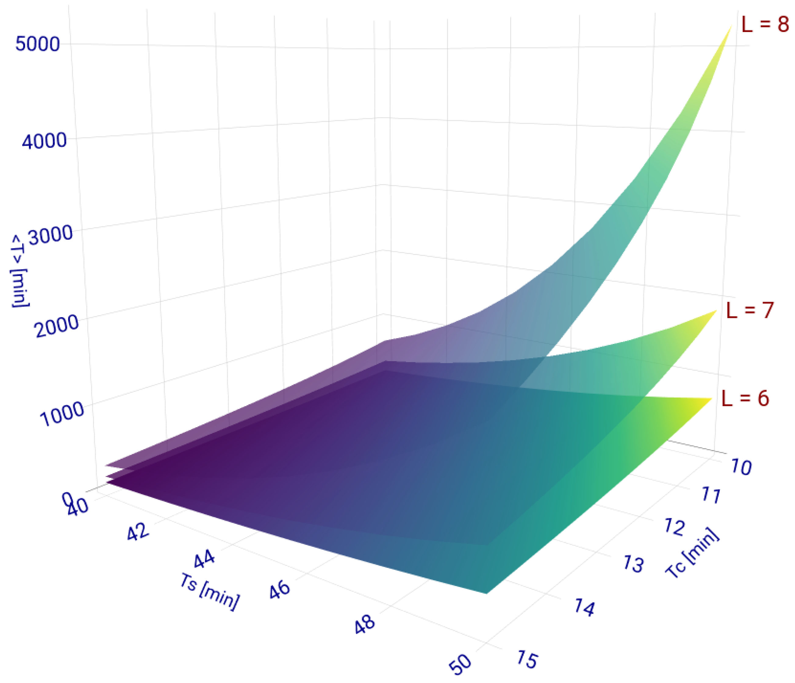
In Figure 2, we show the non-linear behaviour of $<T>$ as a function of $T_C$ and $T_S$ and its strong dependence on L, as they are derived from Equations (2)–(4).

The non-linear nature of $<T>$ is given by the powers of $\gamma$ in Equation (2) and implies a sensitive dependence of the time to the critical condition on its variables. Thus, on the scale of the figure, variations in the order of one minute in $T_C$ or $T_S$ may represent variations of tens to thousands of minutes in $<T>$. The value of L determines the number of terms in Equations (2) and (3). Therefore, adding or removing a server, with the same values of $T_C$ and $T_S$, can make a substantial change in the value of the average MFPT, as can be seen in Figure 2. The sensitivity of our problem on its parameters is very difficult to grasp intuitively and to predict from past experiences in practice.

The main reason for using the birth and death queueing model ($M/M/L$) is the fact that we can derive the closed-form result given in Section 2. However, the analytical prediction of any performance measure needs to be contrasted with numerical outputs from more realistic scenarios. As an illustration, we take values of inter-arrival and service times measured by the EMS Sistema de Urgencias del Rosafe (URG) [25] in Córdoba, Argentina. URG is one of several private EMS operators in a city of about 1.39 million inhabitants. In 2016, URG operated a fleet of nine ambulances that were usually stationed in predefined parking spots scattered throughout the metropolitan zone. The operating scenario distinguishes several daily time bands within which the mean values $T_C$ and $T_S$ are relatively constant, although these, in turn, show seasonal changes throughout the year.

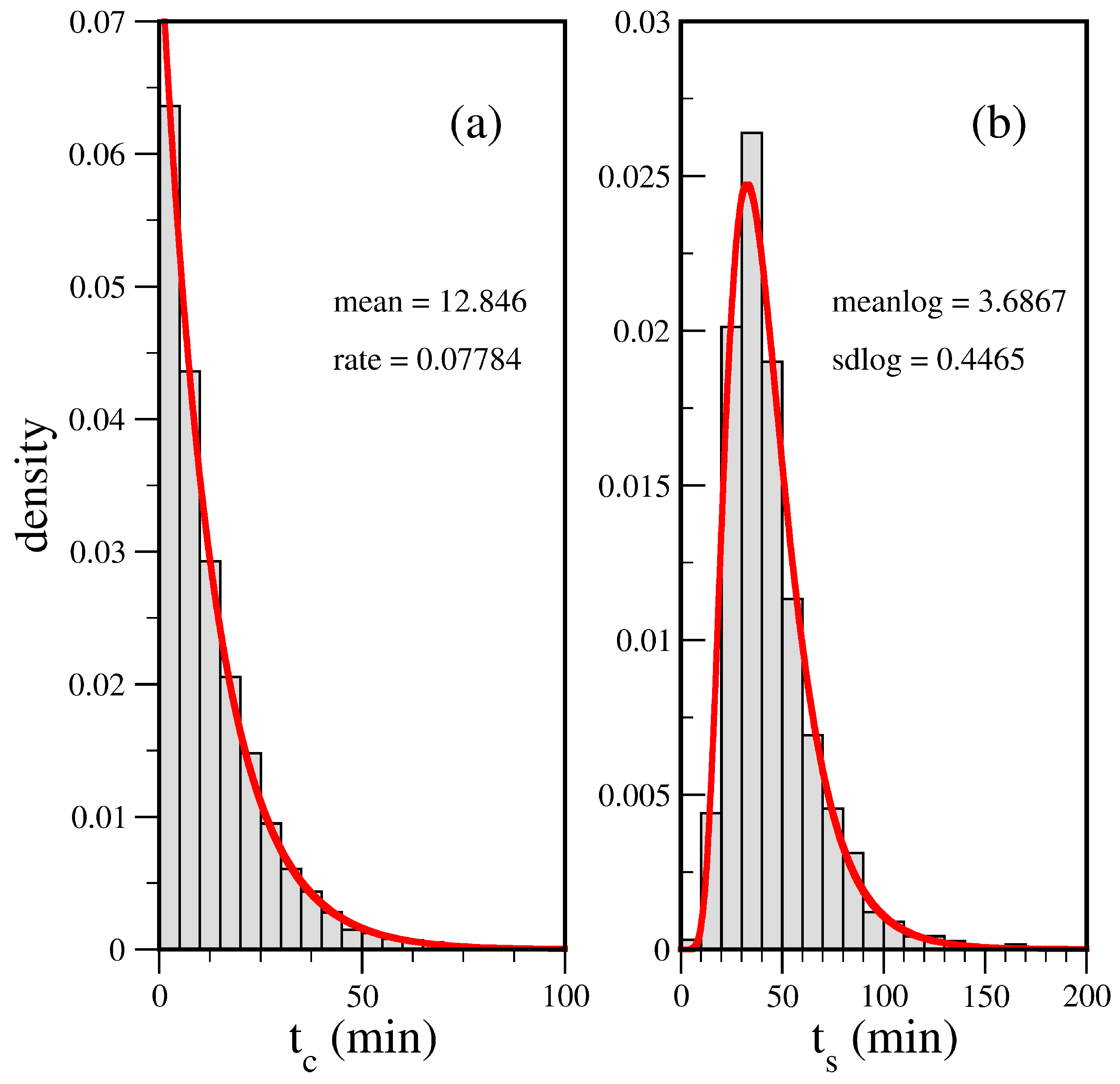
In Figure 3, we show histograms of real data corresponding to 2568 calls received by URG between May 1 and October 31, 2016, late evening (20:00 to 23:00 h). In this time period, we found good stationary statistics in the data, and no critical condition was reported in which there were no ambulances available to serve a call. The service time value measures the time elapsed from dispatch until the ambulance is released. Very low service times correspond to situations that were quickly resolved at scenes close to the ambulance base, whereas the distribution tail involves complex cases with the transfer of the patient to a hospital.

From the figure, we can see that the inter-arrival times fit perfectly with an exponential distribution ($T_C=12.85$ min, goodness-of-fit tests: Kolmogorov–Smirnov p-value $=0.73$, Cramer–von Mises p-value $=0.75$), but the best fit for service times is with a lognormal distribution ($T_S=44.1$ min, goodness-of-fit tests: Kolmogorov–Smirnov p-value $=0.017$, Cramer–von Mises p-value $=0.052$). Thus, in this case, it is apparent that the main limitation of our analytical model is the assumption that the distribution of service times is exponential.

The input traffic to a call centre is a nonstationary Poisson process [7,14,26]. However, the arrival rate function $\lambda \left(t\right)$ is roughly constant over periods of a few hours [11,14,16,27]. Lognormal distributions for service times have already been reported in the literature [12,14,15,16]. The fact that the distribution of the sum of a few independent, but not necessarily identical, lognormal random variables could be approximated by a lognormal distribution [28] may explain the experimental findings when we only use two fitting parameters.

In

Table 1. Comparison among analytic and simulated values of MFPT (in minutes) for a system with seven servers. The simulated values are reported with its standard error for 10,000 simulations. In both cases, the mean service time is $T_S=44.1$ min, whereas, in the first case, the probability distribution of service time is exponential, and in the second case, it is lognormal with meanlog $=3.6867$ and sdlog$=0.4465$. The percentage errors are that of the simulated values with respect to the analytical predictions.

${\mathit{T}}_{\mathit{C}}=\mathbf{5}$min
Initial	Exponential			Lognormal
State	Analytic	Simulated	$\mathit{\epsilon }$%	Simulated	$\mathit{\epsilon }$%
0	67.6	67.2 ± 0.4	0.6	49.8 ± 0.3	35.7
1	62.6	62.2 ± 0.4	0.5	44.8 ± 0.3	39.7
2	57.1	56.7 ± 0.4	0.7	39.8 ± 0.3	43.5
3	50.8	50.5 ± 0.4	0.6	34.7 ± 0.3	46.4
4	43.7	43.4 ± 0.4	0.7	29.4 ± 0.2	48.6
5	35.4	35.1 ± 0.3	0.9	23.7 ± 0.2	49.4
6	25.8	25.4 ± 0.3	1.6	17.1 ± 0.2	50.9
7	14.2	14.1 ± 0.2	0.7	9.3 ± 0.2	52.7
${\mathit{T}}_{\mathit{C}}=\mathbf{10}$min
Initial	Exponential			Lognormal
State	Analytic	Simulated	$\mathbf{\epsilon }$%	Simulated	$\mathbf{\epsilon }$%
0	315.2	310.9 ± 2.5	1.4	244.2 ± 2.1	29.1
1	305.2	300.7 ± 2.5	1.5	234.2 ± 2.1	30.3
2	292.9	288.4 ± 2.5	1.6	223.9 ± 2.1	30.8
3	277.3	272.7 ± 2.5	1.7	212.0 ± 2.1	30.8
4	256.7	252.3 ± 2.5	1.7	197.7 ± 2.1	29.8
5	228.1	224.3 ± 2.5	1.7	176.9 ± 2.0	28.9
6	185.6	182.1 ± 2.4	1.9	145.6 ± 2.0	27.5
7	117.7	115.2 ± 2.0	2.2	92.1 ± 1.7	27.8
${\mathit{T}}_{\mathit{C}}=\mathbf{15}$min
Initial	Exponential			Lognormal
State	Analytic	Simulated	$\mathbf{\epsilon }$%	Simulated	$\mathbf{\epsilon }$%
0	1378.4	1380 ± 13	0.1	1201 ± 12	14.8
1	1363.4	1365 ± 13	0.1	1186 ± 12	15.0
2	1343.3	1345 ± 13	0.1	1169 ± 12	14.9
3	1314.6	1317 ± 13	0.2	1147 ± 12	14.6
4	1270.4	1272 ± 13	0.1	1114 ± 12	14.0
5	1195.1	1198 ± 13	0.2	1056 ± 12	13.2
6	1052.2	1058 ± 12	0.5	937 ± 12	12.3
7	745.4	751 ± 12	0.7	670 ± 11	11.3

, we show a comparison between analytical results given by Equation (2) and simulated MFPT from each initial state of a system with seven servers to the critical condition. The simulations were performed using the fitted distributions in Figure 3 and also using an exponential distribution for service times with a mean value equal to that of the fitted distribution in the right panel.

The analytical predictions agree perfectly with the simulations for the exponentially distributed service times in all cases. For the lognormal distribution of service times, the deviations between the prediction and simulation are about $50\%$ in the worst situations. However, these cases are of little practical interest. Given a fixed number of servers, low values of $T_C$ imply very low MFPT values that are incompatible with EMS response times, while situations with very high values of MFPT are often related with idle infrastructure, which are also avoided in practice.

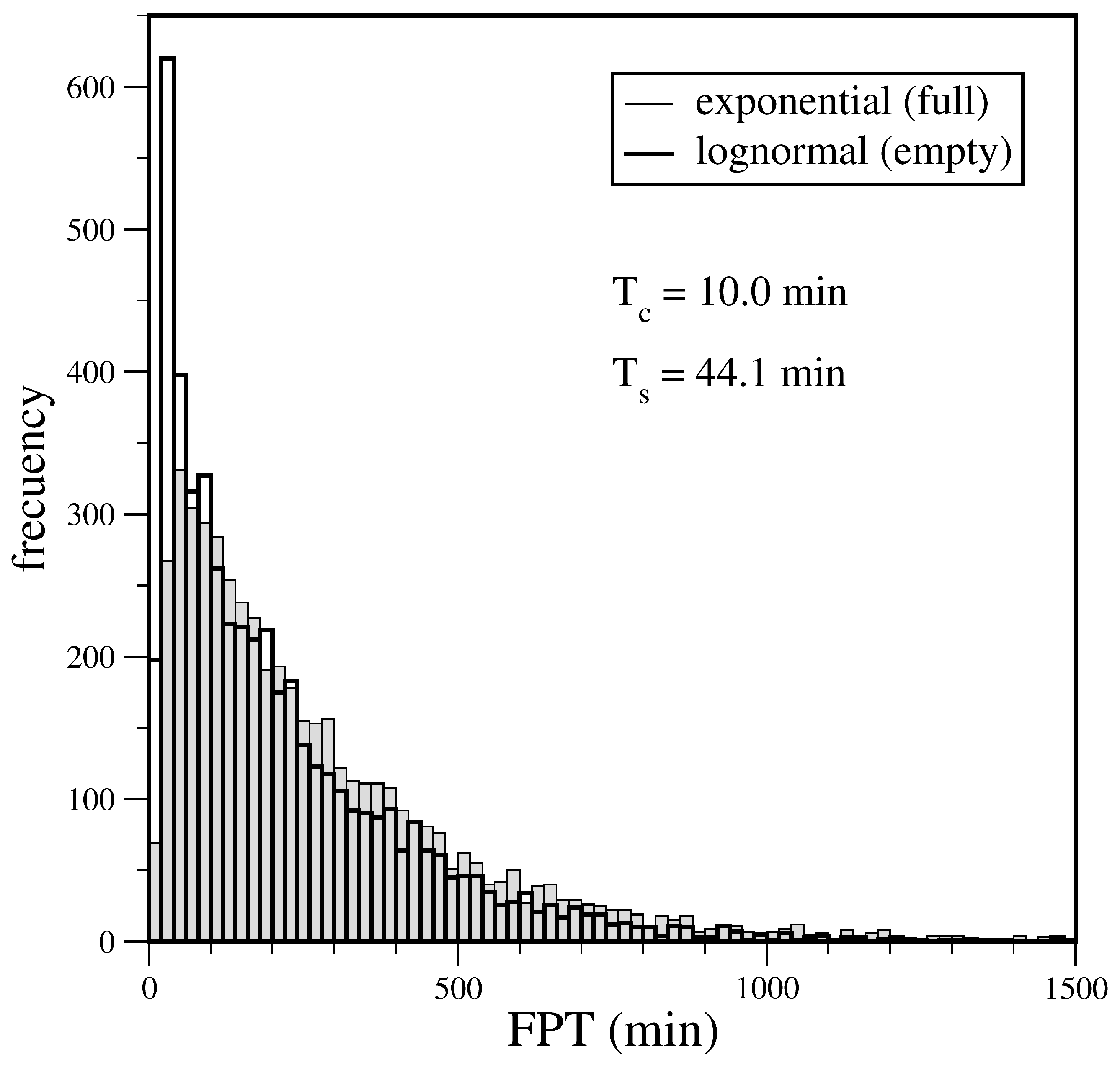
In order to study the differences in the values of FPT under different service time distributions, in Figure 4, we superimpose two histograms of simulated values for a system with seven servers. Both cases correspond to an initial condition with four occupied servers and the same exponential inter-arrival time distribution, but we use two different service time distributions with the same mean value. The FPT distribution with exponential service times is broader than the lognormal counterpart. Therefore, the MFPT under these conditions is shorter for the lognormal service time distribution (also see entry for initial state equal to 4 in Table 1).

Now, we investigate what happens with the residence probabilities in the long time limit. The analytical result given by the Erlang formula has been proven for systems without queue or $M/G/L$ blocking systems [19,20]. That is, if every server is busy when a call arrives, the call is lost; however, it is instructive to analyse the situation of a system with queue. The probability of residence in the queue, $P(n>L)$, is equivalent to the probability absorbed in the site $L+1$ of the Markov chain. From Equation (A11), we can see that the probabilities in Equation (4) are the renormalized residence probabilities of a system with a queue in the interval [0,L]. To find out if this is also the case for lognormal service time distributions, we run our simulator ${10}^7$ min in order to visit each state several times. In the first column of

Table 2. Comparison among analytic and simulated long-run probabilities of residence in each state of a system with seven servers, where q denotes the state with queued calls. All simulations correspond with a simulated running time of $1\times {10}^7$ min. In all cases, $T_C=10$ min and $T_S=44.1$ min, but the parameters in of the lognormal distributions are given by the pairs (meanlog, sdlog): (a) $(3.75521,0.25)$, (b) $(3.59115,0.625)$ and (c) $(3.28646,1.0)$. See Figure 6b.

State	Analytic	Exponential	Lognorm (a)	lognorm (b)	lognorm (c)
0	0.012	0.011	0.011	0.011	0.012
1	0.051	0.050	0.049	0.050	0.052
2	0.112	0.112	0.109	0.111	0.113
3	0.165	0.165	0.164	0.164	0.165
4	0.182	0.182	0.184	0.182	0.181
5	0.160	0.160	0.167	0.163	0.158
6	0.118	0.118	0.127	0.122	0.115
7	0.074	0.074	0.085	0.081	0.075
q	0.126	0.127	0.104	0.114	0.130

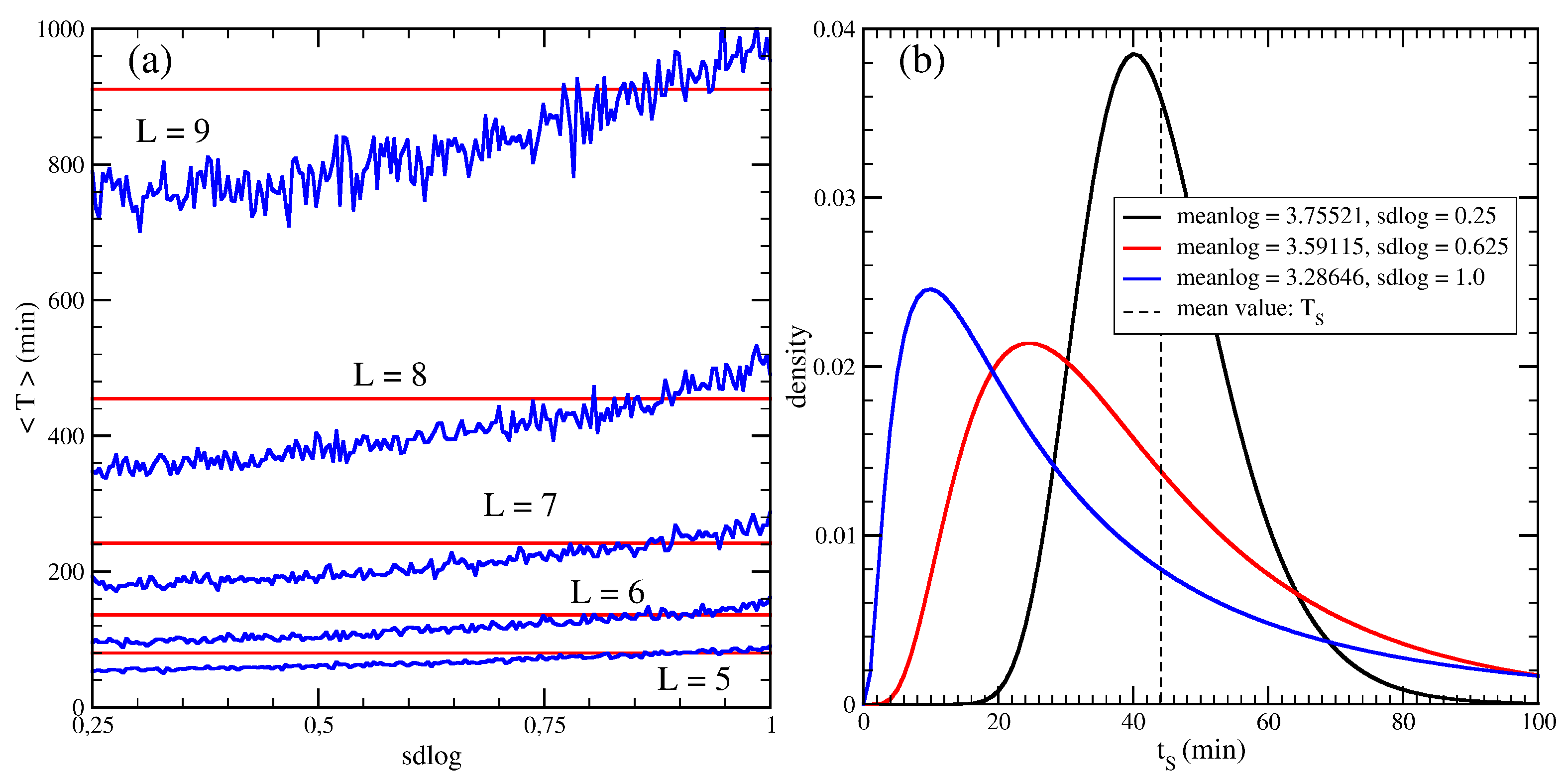
, we show the analytic result of Equations (A11)–(A13) and compare this prediction with the simulated values using four different service time distributions: an exponential and three different lognormal service time distributions—all of these with the same value $T_S=44.1$ min ($T_C=10$ min in all cases). The value sdlog = 0.25 corresponds to the almost symmetric case of the lognormal distribution, and sdlog = 1 corresponds to the more asymmetric situation (see Figure 6b). The exponential distribution is the case completely asymmetric, where the distribution does not have a maximum value. For comparison, we also introduce the middle value sdlog$=0.625$.

The difference among analytical and simulated values are less than $5\%$ in all states with the exception of the queue. The analysed case with queue is a worse situation than the finite chain with both reflecting ends, used in the derivation of Equation (4), because of the probability of residence in the queue may be greater than the saturated state. Therefore, we find it is valid to use the analytic result of Equation (4) for taking the average in Equation (3) and also in the simulation of MFPT with lognormal service time distributions in a system with queue.

In Figure 5, we show the plots of MFPT averaged over the initial conditions, $<T>$, as a function of the mean inter-arrival time $T_C$ using the probabilities given by Equation (4). We have sketched a characteristic situation for the service time, and we considered several numbers of servers $L=5,\cdots ,9$. The curves clearly show the non-linear behaviour of $<T>$ and allow us to evaluate the quality of the fit for the simulated situations achieved with our analytical expression.

Again, in the left panel, we find excellent agreement among the analytical predictions and the simulations for exponentially distributed service times. In contrast, in the right panel, for lognormal distributed service times, we see that the analytical curves always run over the corresponding simulation. This fact has just been seen in Figure 4, where the FPT distribution has a longer tail in the case of service times distributed exponentially with respect to lognormal service times. Thus, the mean value of the FPT distribution (MFPT) is higher for exponential service times. Therefore, the analytic model underestimates the number of necessary servers under a given stress condition. Drawing a horizontal line in Figure 5b, when we move in the direction of increasing demand (that is, lowering $T_C$), we first cross the blue (simulated) curves in all the considered cases. This is an important fact to keep in mind if we want to use the analytical model to find the best number of servers in a particular operational scenario. However, the discrepancies observed between the simulations and the closed form expression for the average MFPT are not significant enough to cause a considerable effect in the estimation of the optimal number of servers, given the separation among the curves for different values of L. Thus, for example, from Figure 5b, we can see that to obtain an average MFPT of 6 hs, given $T_C=14$ min, six servers are needed, whereas for $T_C=10$, eight servers are needed under the same service conditions.

We also analyse the effect of asymmetry in the service time distribution on average MFPT. For this purpose, we simulate the average MFPT for a whole family of service time distribution with fixed $T_S$ but changing the parameter sdlog in the interval $[0.25,1]$, where the minimum value corresponds to the almost symmetric case and the maximum corresponds to the more asymmetric situation. The average MFPT as a function of the sdlog parameter is shown in Figure 6.

In all cases, the analytical prediction gives an acceptable approximation for the simulated data.

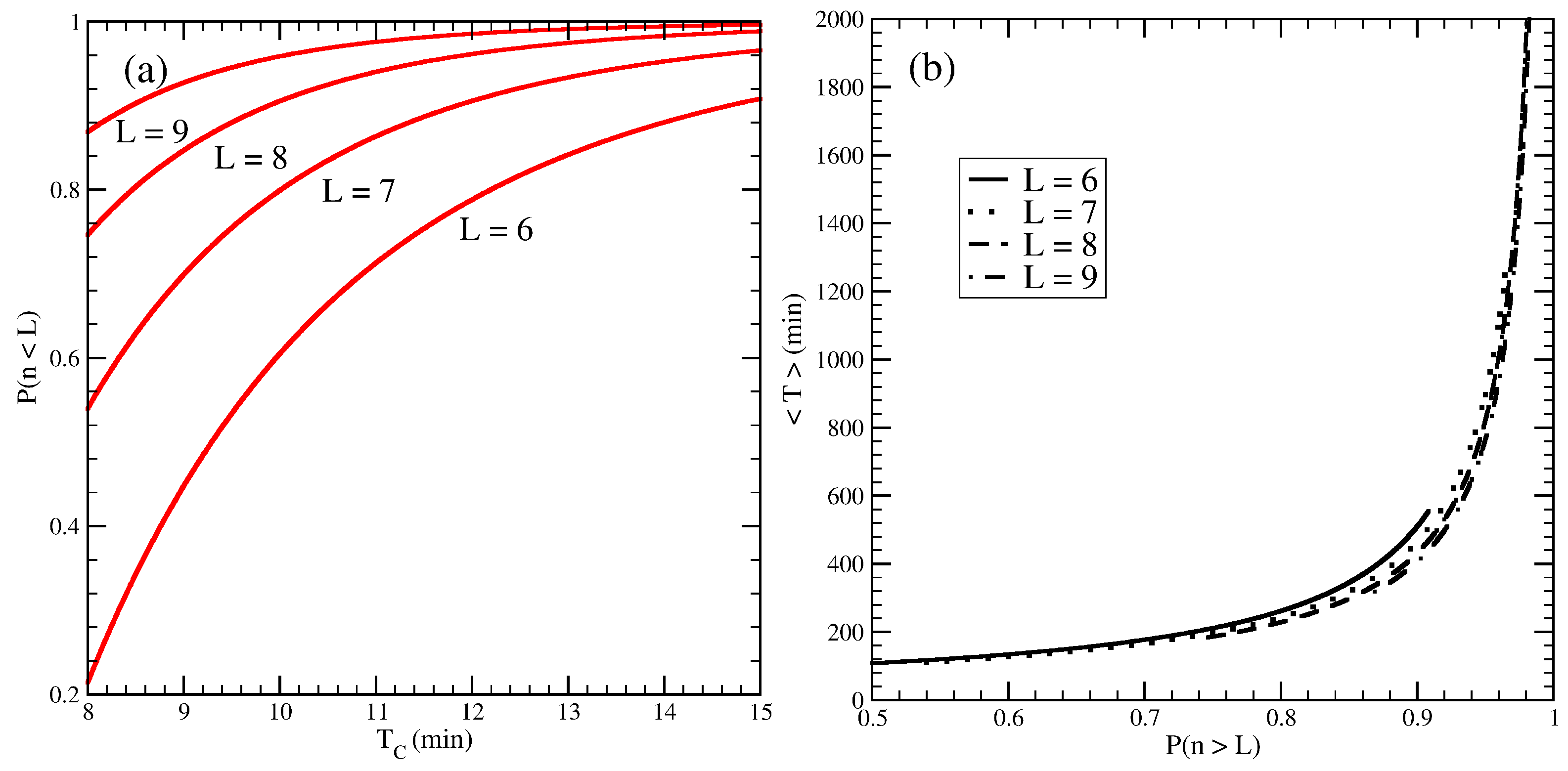
Finally, in the left panel of Figure 7, we plot the probability that one or more servers are available at the instant of a emergency call, $P(n<L)$ [27], as a function of the time between calls for a fixed mean service time. We are using Equation (4) for the calculation of this probability. In the right panel, we plot the average MFPT as a function of this availability probability for the same values of $T_C$ given in the left panel. We can observe a very strong sensitivity of the average MFPT to the availability probability for high values of system availability. Thus, only controlling the availability of the system is not enough to assure a long enough time to the critical condition. A dispatcher observing a high availability probability value might conclude that the system is running unreasonably idle; however, the time to critical condition may be shorter than the expectation. More interesting, however, is that the function $<T>$ vs. $P(n<L)$ is practically independent of the number of servers.

4. Concluding Remarks

MFPT is a useful KPI that allows estimating the running operative lapse of a system, under a given stress condition, before a service disruption. In this work, we have presented a closed-form expression to calculate the MFPT for a system of servers in parallel, and we also provide a simulation framework for the MFPT. Our formula, based on a birth–death process, only uses the average time between demands and the average service time. Our results make it possible to predict the MFPT given the stress of the system at a particular moment or to analyse the servers shortage time under generic operating conditions by averaging over the initial states of the system. The main limitation of our results, as is often with analytical exact results in queueing theory, is the assumption of an exponential distribution for service times. The impact of this limiting assumption is confronted with results of simulations using more realistic service distributions. Our results indicate that our analytical formula is an acceptable approximation under practical situations. Interesting potential future work may be to consider the implementation of accurate approximations for the M/G/L problem [29] to the MFPT calculation. In addition, our simulation scheme allows us to evaluate the MFPT in any $GI/G/L/FCFS$ server configuration.