Spherical Fuzzy Graphs with Application to Decision-Making

Abstract

In a network model, the evaluation information given by decision makers are occasionally of types: yes, abstain, no, and refusal. To deal with such problems, we use mathematical models based on picture fuzzy sets. The spherical fuzzy model is more versatile than the picture fuzzy model as it broadens the space of uncertain and vague information, due to its outstanding feature of vast space of participation of acceptable triplets. Graphs are a mathematical representation of networks. Thus to deal with many real-world phenomena represented by networks, spherical fuzzy graphs can be used to model different practical scenarios in a more flexible manner than picture fuzzy graphs. In this research article, we discuss two operations on spherical fuzzy graphs (SFGs), namely, symmetric difference and rejection; and develop some results regarding their degrees and total degrees. We describe certain concepts of irregular SFGs with several important properties. Further, we present an application of SFGs in decision making.

1. Introduction

Fuzzy set theory proposed by Zadeh [1] is an extension of classical set theory. Zadeh’s remarkable idea has found many applications in several fields, including chemical industry, telecommunication, decision theory, networking, computer science, and management science. Atanassov [2] introduced the intuitionistic fuzzy set (IFS) as an extension of fuzzy set (FS) theory. He broadened the idea of FSs by defining the truthness degree $\left(\alpha \right)$ alongside the falseness degree $\left(\beta \right)$ with the requirement $0\le \alpha +\beta \le 1.$ Fortifying the idea of IFS, Yager [3] proposed Pythagorean fuzzy sets (PyFS), which broadened the space of participation by presenting a new limitation, $0\le {\alpha }^2+{\beta }^2\le 1.$

Cuong [4,5] initiated the concept of the picture fuzzy set (PFS) as a direct extension of intuitonistic fuzzy sets, which may be adequate in cases when human opinions are of types: yes, abstain, no, and refusal. A picture fuzzy set gives three degrees to the elements named truthness degree $\alpha :X\to [0,1],$ abstinence degree $\gamma :X\to [0,1]$, and falseness degree $\beta :X\to [0,1]$ under the condition $0\le \alpha +\gamma +\beta \le 1,$ where $\pi =1-(\alpha +\gamma +\beta )$ is the refusal degree. PFSs have many applications in fuzzy inference, clustering, decision making etc.

Zeng et al. [6] explored the picture fuzzy divergence measure in multi-criteria group decision making. Garg [7] presented some picture fuzzy aggregation operators. Recently, Liu et al. [8] defined picture fuzzy weighted distance measures and their application to investment selection. Zhang et al. [9] explored picture fuzzy Dombi Heronian mean operators. For further study on picture fuzzy sets, one may refer to [10,11,12,13,14,15].

The spherical fuzzy set (SFS), proposed by Gündogdu and Kahraman [16], is an extension of PFS, as it provides enlargement of the space of degrees of truthness $\left(\alpha \right),$ abstinence $\left(\gamma \right)$, and falseness $\left(\beta \right)$ in the interval $[0,1]$ with a condition $0\le {\alpha }^2+{\gamma }^2+{\beta }^2\le 1.$ Ashraf et al. [17] presented the notion of SFSs with applications in decision making problems. Another extension suggested by Li et al. [18] in 2018 is the q-rung picture fuzzy set (q-RPFS). The proposed concept relaxes the constraints of picture and spherical fuzzy sets with $0\le {\alpha }^q+{\gamma }^q+{\beta }^q\le 1,q\ge 1.$ This model can express vague information more flexibly and accurately with increasing q rungs.

Graph theory has become a powerful conceptual framework for modeling and for solutions of combinatorial problems that arise in various areas, including mathematics, computer science, and engineering. Many real life problems can be represented by graphs. Graph theory was first presented by Euler, when he handled Königsberg’s bridges problem. Kaufmann [19] proposed the notion of fuzzy graphs (FG) based on Zadeh’s fuzzy relation [20]. Rosenfeld [21] developed the structure of FGs by obtaining various fuzzy analogs of graph theoretic concepts such as cycles, paths, and connectedness. After that, Bhattacharya [22] discussed some remarks on FGs with a demonstration that every idea in classical graph theory does not have equivalence in FGs.

As the concept of regularity led to many developments in the structural theory of graphs, meanwhile, the irregular graphs have also been significant while dealing with network heterogeneity, which has many applications across ecology, biology, economy, and technology. Literature shows that many researchers have studied this property for fuzzy graphs and its extensions. Santhimaheswari and Sekar [23] discussed strongly edged irregular and totally irregular FGs. Al-Hawary [24,25,26,27] considered certain notions of fuzzy graphs. Parvathi and Karunambigai [28] extended the theory of FGs to intuitionistic fuzzy graphs (IFGs). Afterward, IFGs were examined by Akram and Davvaz [29]. Naz et al. [30] presented the notion of Pythagorean fuzzy graphs (PyFGs), an extension of the concept of Akram and Davvaz’s IFGs, including its applications in decision-making. Akram et al. [31] described the specific types of PyFGs and their applications to decision-making. Recently, Akram [32] investigated decision making methods based on spherical fuzzy graphs. Akram and Habib [33,34] introduced the concept of q-RPFGs and discussed their regularity. Some decision making approaches based on modified VIKOR and TOPSIS methods can be seen in [35,36]. For further study on these graphs, one may refer to [37,38,39,40].

The spherical fuzzy model is a more versatile model, as it tackles the ambiguities in real phenomena in a broad manner. To deal with many real world issues and to relax the bounding constraint, the implication to the necessity of SFGs arises. The objective of this study is to expand the graph-theoretic concepts under a SF environment. In this research article, we discuss two operations on SFGs namely, symmetric difference and rejection with a brief description on degree and total degree of SFGs, along with some related results. We develop several properties of irregular and edge-irregular SFGs with examples. Further, we describe an application of SFGs in the decision making process.

2. Spherical Fuzzy Graphs

Definition 1

([16]). A spherical fuzzy set X on an underlying set V is defined as

$$X=\left\{(a,{\alpha }_X\left(a\right),{\gamma }_X\left(a\right),{\beta }_X\left(a\right))\right|a\in V\}$$

where ${\alpha }_X\left(a\right)\in [0,1]$ is known as the degree of truthness of a in X, ${\gamma }_X\left(a\right)\in [0,1]$ is known as the degree of abstinence of a in X, and ${\beta }_X\left(a\right)\in [0,1]$ is known as the degree of falseness of a in X, where ${\alpha }_X,{\gamma }_X\mathrm{and}{\beta }_X$ fulfil the following condition $0\le {\alpha }_X^2\left(a\right)+{\gamma }_X^2\left(a\right)+{\beta }_X^2\left(a\right)\le 1.$ Further, for all $a\in V,{\delta }_X\left(a\right)=\sqrt{1-({\alpha }_X^2\left(a\right)+{\gamma }_X^2\left(a\right)+{\beta }_X^2\left(a\right))}$ is called the degree of refusal of membership of a in X.

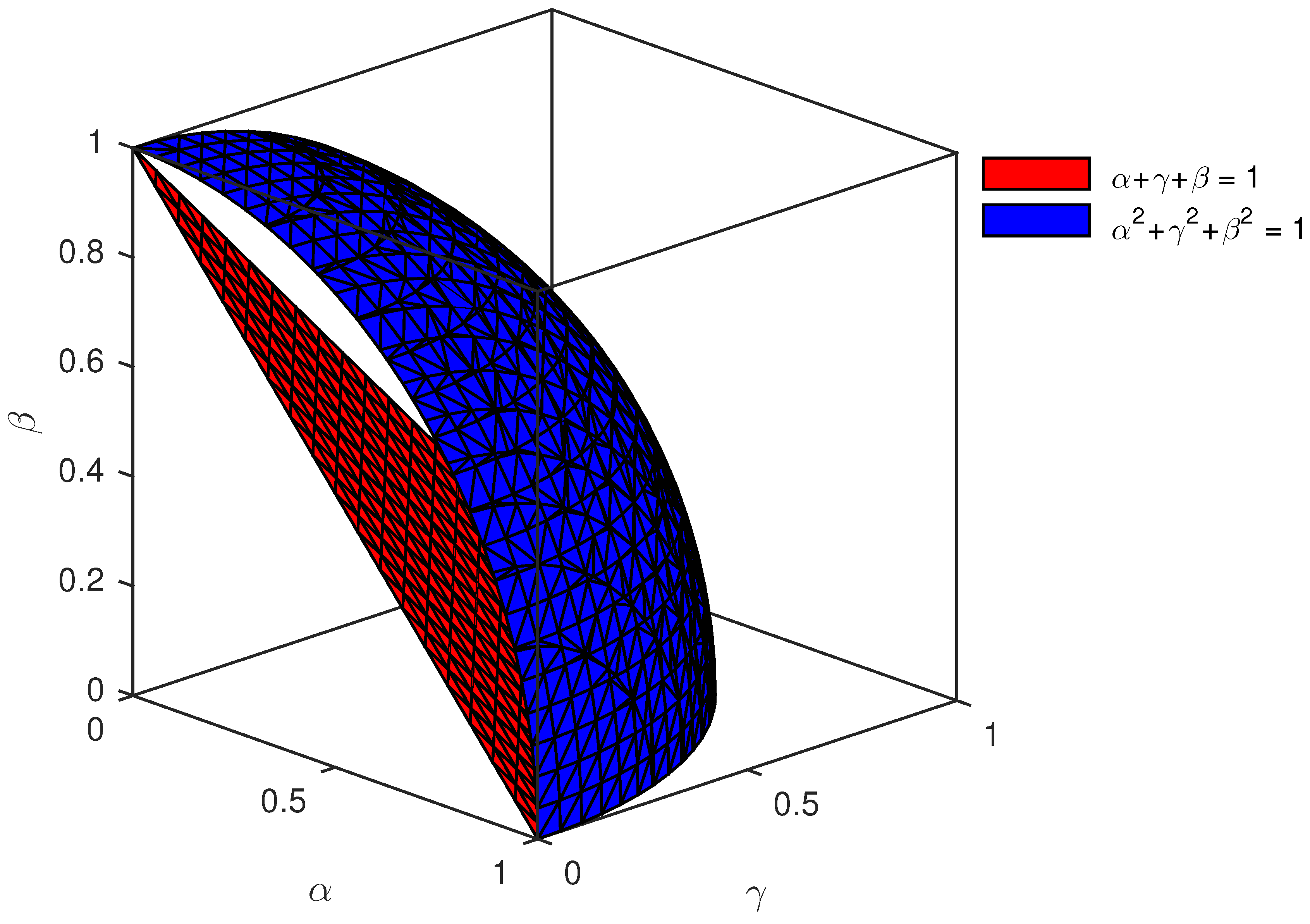
Figure 1 compares the spaces of spherical fuzzy sets and picture fuzzy sets.

Definition 2.

A spherical fuzzy graph (SFG) on an underlying set V is a pair $\mathcal{G}=(M,N),$ where M is a spherical fuzzy set in V and N is a spherical fuzzy relation on $V\times V$, such that

$$\begin{array}{cc}\hfill {\alpha }_N(a,b)& \le min\{{\alpha }_M\left(a\right),{\alpha }_M\left(b\right)\},\hfill \\ \hfill {\gamma }_N(a,b)& \le min\{{\gamma }_M\left(a\right),{\gamma }_M\left(b\right)\},\hfill \\ \hfill {\beta }_N(a,b)& \le max\{{\beta }_M\left(a\right),{\beta }_M\left(b\right)\},\hfill \end{array}$$

where α is known as the degree of truthness, γ is known as the degree of abstinence, and β is known as the degree of falseness and fulfils the following condition $0\le {\alpha }_N^2(a,b)+{\gamma }_N^2(a,b)+{\beta }_N^2(a,b)\le 1$ for all $a,b\in V,$ where M is a spherical fuzzy vertex set and N is a spherical fuzzy edge set of$\mathcal{G}$.

Definition 3.

Let $\mathcal{G}=(M,N)$ be an SFG defined on $G^{*}=(V,E).$ The degree of a vertex a of $\mathcal{G}$ is denoted by $d_{\mathcal{G}}\left(a\right)=(d_{\alpha }\left(a\right),d_{\gamma }\left(a\right),d_{\beta }\left(a\right))$ and defined as

$$d_{\mathcal{G}}\left(a\right)=\left(\sum _{a\ne b}{\alpha }_Y(a,b),\sum _{a\ne b}{\gamma }_Y(a,b),\sum _{a\ne b}{\beta }_Y(a,b)\right)$$

for all$(a,b)\in E.$

Definition 4.

Let $\mathcal{G}=(M,N)$ be an SFG defined on $G^{*}=(V,E).$ The total degree of a vertex a of $\mathcal{G}$ is denoted by $t{d}_{\mathcal{G}}\left(a\right)=(t{d}_{\alpha }\left(a\right),t{d}_{\gamma }\left(a\right),t{d}_{\beta }\left(a\right))$ and defined as

$$t{d}_{\mathcal{G}}\left(a\right)=\left(\sum _{a\ne b}{\alpha }_Y(a,b)+{\alpha }_X\left(a\right),\sum _{a\ne b}{\gamma }_Y(a,b)+{\gamma }_X\left(a\right),\sum _{a\ne b}{\beta }_Y(a,b)+{\beta }_X\left(a\right)\right)$$

for all$(a,b)\in E.$

We now define two operations: symmetric difference and rejection on spherical fuzzy graphs, and develop several important results.

Definition 5.

Let $M_1=({\alpha }_{M_1},{\gamma }_{M_1},{\beta }_{M_1})$ and $M_2=({\alpha }_{M_2},{\gamma }_{M_2},{\beta }_{M_2})$ be spherical fuzzy sets defined on $V_1$ and $V_2,$ and let $N_1=({\alpha }_{N_1},{\gamma }_{N_1},{\beta }_{N_1})$ and $N_2=({\alpha }_{N_2},{\gamma }_{N_2},{\beta }_{N_2})$ be spherical fuzzy sets defined on $E_1$ and $E_2$, respectively. Then, we denote the symmetric difference of two SFGs ${\mathcal{G}}_1$ and ${\mathcal{G}}_2$ of the graphs $G_1^{*}$ and $G_2^{*}$ by ${\mathcal{G}}_1\oplus {\mathcal{G}}_2=(M_1\oplus M_2,N_1\oplus N_2),$ and define as follows:

$$\begin{array}{cc}\hfill \left(\mathrm{i}\right)\left({\alpha }_{M_1}\oplus {\alpha }_{M_2}\right)(a_1,a_2)& =min\{{\alpha }_{M_1}\left(a_1\right),{\alpha }_{M_2}\left(a_2\right)\}\hfill \\ \hfill \left({\gamma }_{M_1}\oplus {\gamma }_{M_2}\right)(a_1,a_2)& =min\{{\gamma }_{M_1}\left(a_1\right),{\gamma }_{M_2}\left(a_2\right)\}\hfill \\ \hfill \left({\beta }_{M_1}\oplus {\beta }_{M_2}\right)(a_1,a_2)& =max\{{\beta }_{M_1}\left(a_1\right),{\beta }_{M_2}\left(a_2\right)\}\mathrm{for}\mathrm{all}{a}_1,a_2\in V,\hfill \end{array}$$

$$\begin{array}{cc}\hfill \left(\mathrm{ii}\right)\left({\alpha }_{N_1}\oplus {\alpha }_{N_2}\right)(a,a_2)(a,b_2)& =min\{{\alpha }_{M_1}\left(a\right),{\alpha }_{N_2}\left(a_2{b}_2\right)\}\hfill \\ \hfill \left({\gamma }_{N_1}\oplus {\gamma }_{N_2}\right)(a,a_2)(a,b_2)& =min\{{\gamma }_{M_1}\left(a\right),{\gamma }_{N_2}\left(a_2{b}_2\right)\}\hfill \\ \hfill \left({\beta }_{N_1}\oplus {\beta }_{N_2}\right)(a,a_2)(a,b_2)& =max\{{\beta }_{M_1}\left(a\right),{\beta }_{N_2}\left(a_2{b}_2\right)\}\mathrm{for}\mathrm{all}a\in V_1,\mathrm{for}\mathrm{all}{a}_2{b}_2\in E_2,\hfill \end{array}$$

$$\begin{array}{cc}\hfill \left(\mathrm{iii}\right)\left({\alpha }_{N_1}\oplus {\alpha }_{N_2}\right)(a_1,c)(b_1,c)& =min\{{\alpha }_{N_1}\left(a_1{b}_1\right),{\alpha }_{M_2}\left(c\right)\}\hfill \\ \hfill \left({\gamma }_{N_1}\oplus {\gamma }_{N_2}\right)(a_1,c)(b_1,c)& =min\{{\gamma }_{N_1}\left(a_1{b}_1\right),{\gamma }_{M_2}\left(c\right)\}\hfill \\ \hfill \left({\beta }_{N_1}\oplus {\beta }_{N_2}\right)(a_1,c)(b_1,c)& =max\{{\beta }_{N_1}\left(a_1{b}_1\right),{\beta }_{M_2}\left(c\right)\}\mathrm{for}\mathrm{all}c\in V_2,\mathrm{for}\mathrm{all}{a}_1{b}_1\in E_1,\hfill \end{array}$$

$$\begin{array}{cc}\hfill \left(\mathrm{iv}\right)\left({\alpha }_{N_1}\oplus {\alpha }_{N_2}\right)(a_1,a_2)(b_1,b_2)& =min\{{\alpha }_{M_1}\left(a_1\right),{\alpha }_{M_1}\left(b_1\right),{\alpha }_{N_2}\left(a_2{b}_2\right)\}\mathrm{for}\mathrm{all}{a}_1{b}_1\notin E_1,a_2{b}_2\in E_2\hfill \\ \hfill & \mathrm{or}\hfill \\ \hfill & =min\{{\alpha }_{M_2}\left(a_2\right),{\alpha }_{M_2}\left(b_2\right),{\alpha }_{N_1}\left(a_1{b}_1\right)\}\mathrm{for}\mathrm{all}{a}_2{b}_2\notin E_2,a_1{b}_1\in E_1,\hfill \\ \hfill \left({\gamma }_{N_1}\oplus {\gamma }_{N_2}\right)(a_1,a_2)(b_1,b_2)& =min\{{\gamma }_{M_1}\left(a_1\right),{\gamma }_{M_1}\left(b_1\right),{\gamma }_{N_2}\left(a_2{b}_2\right)\}\mathrm{for}\mathrm{all}{a}_1{b}_1\notin E_1,a_2{b}_2\in E_2\hfill \\ \hfill & \mathrm{or}\hfill \\ \hfill & =min\{{\gamma }_{M_2}\left(a_2\right),{\gamma }_{M_2}\left(b_2\right),{\gamma }_{N_1}\left(a_1{b}_1\right)\}\mathrm{for}\mathrm{all}{a}_2{b}_2\notin E_2,a_1{b}_1\in E_1,\hfill \\ \hfill \left({\beta }_{N_1}\oplus {\beta }_{N_2}\right)(a_1,a_2)(b_1,b_2)& =max\{{\beta }_{M_1}\left(a_1\right),{\beta }_{M_1}\left(b_1\right),{\beta }_{N_2}\left(a_2{b}_2\right)\}\mathrm{for}\mathrm{all}{a}_1{b}_1\notin E_1,a_2{b}_2\in E_2\hfill \\ \hfill & \mathrm{or}\hfill \\ \hfill & =max\{{\beta }_{M_2}\left(a_2\right),{\beta }_{M_2}\left(b_2\right),{\beta }_{N_1}\left(a_1{b}_1\right)\}\mathrm{for}\mathrm{all}{a}_2{b}_2\notin E_2,a_1{b}_1\in E_1.\hfill \end{array}$$

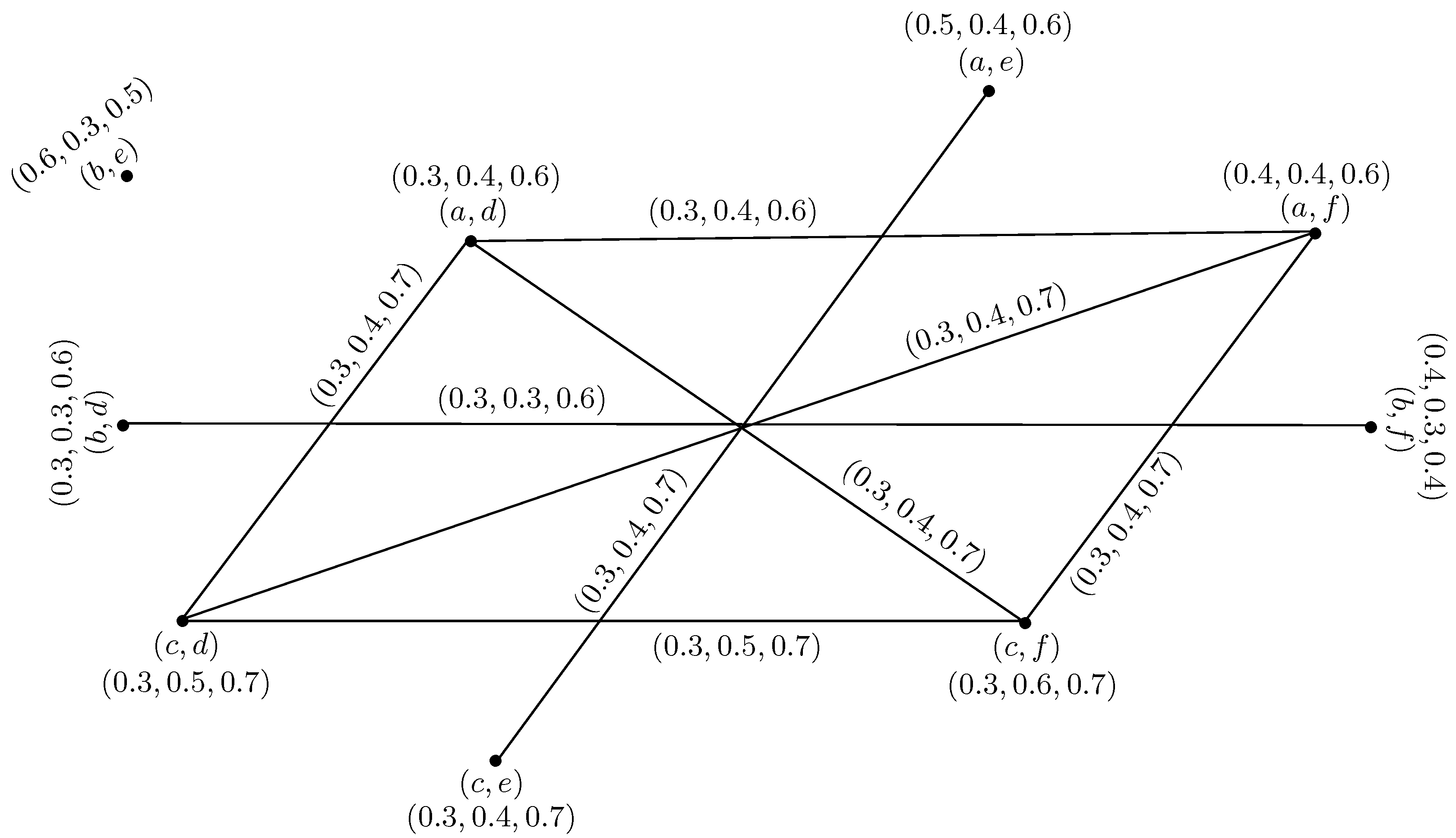
Example 1.

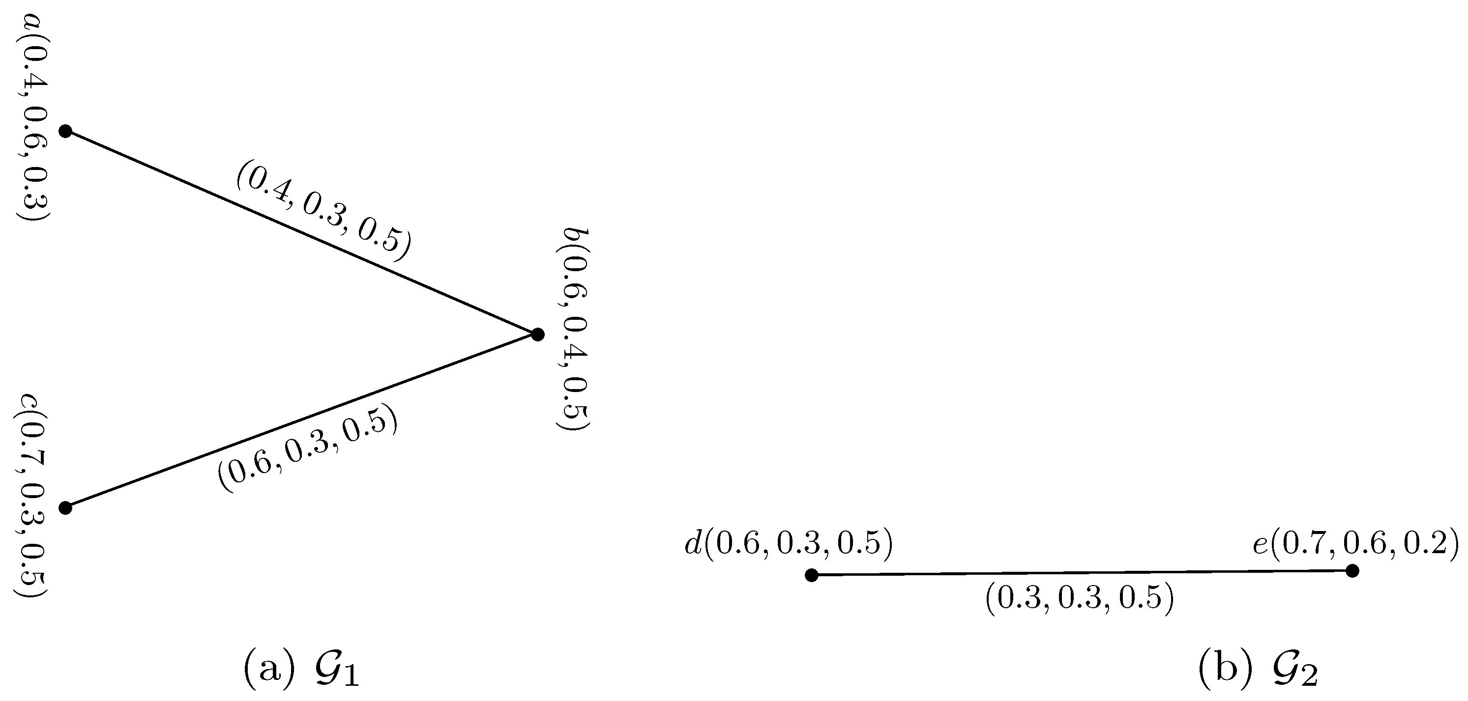
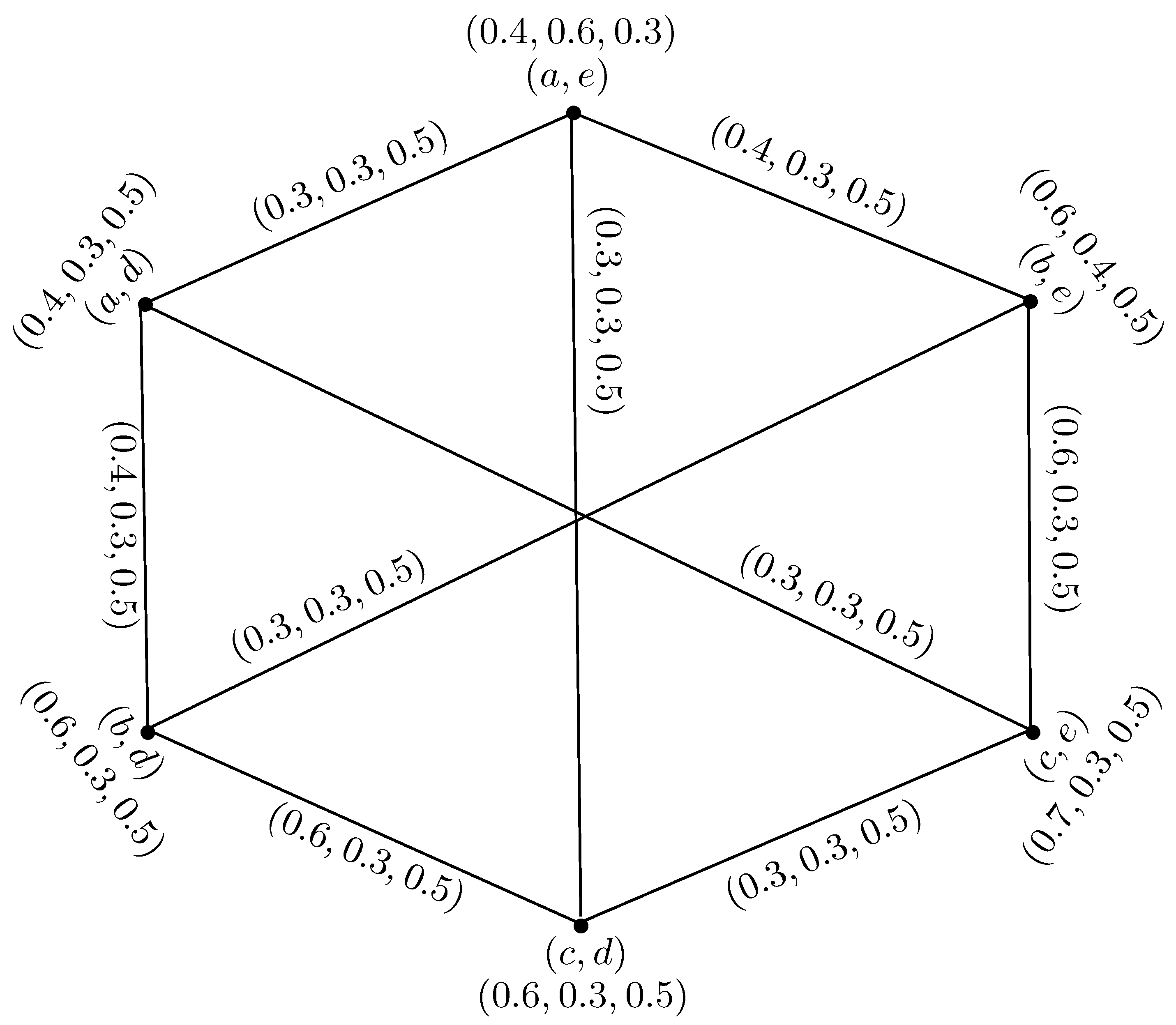
Consider two SFGs ${\mathcal{G}}_1=(M_1,N_1)$ and ${\mathcal{G}}_2=(M_2,N_2)$, as shown in Figure 2. Their symmetric difference ${\mathcal{G}}_1\oplus {\mathcal{G}}_2$ is shown in Figure 3.

Proposition 1.

If ${\mathcal{G}}_1$ and ${\mathcal{G}}_2$ are SFGs, then ${\mathcal{G}}_1\oplus {\mathcal{G}}_2$ is a SFG.

Proof. 

Let $a\in V_1$ and $a_2{b}_2\in E_2$. Then we have

$$\begin{array}{cc}\hfill \left({\alpha }_{N_1}\oplus {\alpha }_{N_2}\right)(a,a_2)(a,b_2)& =min\left({\alpha }_{M_1}\left(a\right),{\alpha }_{N_2}\left(a_2{b}_2\right)\right)\le min\left({\alpha }_{M_1}\left(a\right),min\left({\alpha }_{M_2}\left(a_2\right),{\alpha }_{M_2}\left(b_2\right)\right)\right)\hfill \\ \hfill & =min\left(min\left({\alpha }_{M_1}\left(a\right),{\alpha }_{M_2}\left(a_2\right)\right),min\left({\alpha }_{M_1}\left(a\right),{\alpha }_{M_2}\left(b_2\right)\right)\right)\hfill \\ \hfill & =min\left(\left({\alpha }_{M_1}\oplus {\alpha }_{M_2}\right)(a,a_2),\left({\alpha }_{M_1}\oplus {\alpha }_{M_2}\right)(a,b_2)\right),\hfill \end{array}$$

$$\begin{array}{cc}\hfill \left({\gamma }_{N_1}\oplus {\gamma }_{N_2}\right)(a,a_2)(a,b_2)& =min\left({\gamma }_{M_1}\left(a\right),{\gamma }_{N_2}\left(a_2{b}_2\right)\right)\le min\left({\gamma }_{M_1}\left(a\right),min\left({\gamma }_{M_2}\left(a_2\right),{\gamma }_{M_2}\left(b_2\right)\right)\right)\hfill \\ \hfill & =min\left(min\left({\gamma }_{M_1}\left(a\right),{\gamma }_{M_2}\left(a_2\right)\right),min\left({\gamma }_{M_1}\left(a\right),{\gamma }_{M_2}\left(b_2\right)\right)\right)\hfill \\ \hfill & =min\left(\left({\gamma }_{M_1}\oplus {\gamma }_{M_2}\right)(a,a_2),\left({\gamma }_{M_1}\oplus {\gamma }_{M_2}\right)(a,b_2)\right),\hfill \end{array}$$

$$\begin{array}{cc}\hfill \left({\beta }_{N_1}\oplus {\beta }_{N_2}\right)(a,a_2)(a,b_2)& =max\left({\beta }_{M_1}\left(a\right),{\beta }_{N_2}\left(a_2{b}_2\right)\right)\le max\left({\beta }_{M_1}\left(a\right),max\left({\beta }_{M_2}\left(a_2\right),{\beta }_{M_2}\left(b_2\right)\right)\right)\hfill \\ \hfill & =max\left(max\left({\beta }_{M_1}\left(a\right),{\beta }_{M_2}\left(a_2\right)\right),max\left({\beta }_{M_1}\left(a\right),{\beta }_{M_2}\left(b_2\right)\right)\right)\hfill \\ \hfill & =max\left(\left({\beta }_{M_1}\oplus {\beta }_{M_2}\right)(a,a_2),\left({\beta }_{M_1}\oplus {\beta }_{M_2}\right)(a,b_2)\right).\hfill \end{array}$$

Let $c\in V_2$ and $a_1{b}_1\in E_1$. Then we have

$$\begin{array}{cc}\hfill \left({\alpha }_{N_1}\oplus {\alpha }_{N_2}\right)(a_1,c)(b_1,c)& =min\left({\alpha }_{N_1}\left(a_1{b}_1\right),{\alpha }_{M_2}\left(c\right)\right)\le min\left(min\left({\alpha }_{M_1}\left(a_1\right),{\alpha }_{M_1}\left(b_1\right)\right),{\alpha }_{M_2}\left(c\right)\right)\hfill \\ \hfill & =min\left(min\left({\alpha }_{M_1}\left(a_1\right),{\alpha }_{M_2}\left(c\right)\right),min\left({\alpha }_{M_1}\left(b_1\right),{\alpha }_{M_2}\left(c\right)\right)\right)\hfill \\ \hfill & =min\left(\left({\alpha }_{M_1}\oplus {\alpha }_{M_2}\right)(a_1,c),\left({\alpha }_{M_1}\oplus {\alpha }_{M_2}\right)(b_1,c)\right),\hfill \end{array}$$

$$\begin{array}{cc}\hfill \left({\gamma }_{N_1}\oplus {\gamma }_{N_2}\right)(a_1,c)(b_1,c)& =min\left({\gamma }_{N_1}\left(a_1{b}_1\right),{\gamma }_{M_2}\left(c\right)\right)\le min\left(min\left({\gamma }_{M_1}\left(a_1\right),{\gamma }_{M_1}\left(b_1\right)\right),{\gamma }_{M_2}\left(c\right)\right)\hfill \\ \hfill & =min\left(min\left({\gamma }_{M_1}\left(a_1\right),{\gamma }_{M_2}\left(c\right)\right),min\left({\gamma }_{M_1}\left(b_1\right),{\gamma }_{M_2}\left(c\right)\right)\right)\hfill \\ \hfill & =min\left(\left({\gamma }_{M_1}\oplus {\gamma }_{M_2}\right)(a_1,c),\left({\gamma }_{M_1}\oplus {\gamma }_{M_2}\right)(b_1,c)\right),\hfill \end{array}$$

$$\begin{array}{cc}\hfill \left({\beta }_{N_1}\oplus {\beta }_{N_2}\right)(a_1,c)(b_1,c)& =max\left({\beta }_{N_1}\left(a_1{b}_1\right),{\beta }_{M_2}\left(c\right)\right)\le max\left(max\left({\beta }_{M_1}\left(a_1\right),{\beta }_{M_1}\left(b_1\right)\right),{\beta }_{M_2}\left(c\right)\right)\hfill \\ \hfill & =max\left(max\left({\beta }_{M_1}\left(a_1\right),{\beta }_{M_2}\left(c\right)\right),max\left({\beta }_{M_1}\left(b_1\right),{\beta }_{M_2}\left(c\right)\right)\right)\hfill \\ \hfill & =max\left(\left({\beta }_{M_1}\oplus {\beta }_{M_2}\right)(a_1,c),\left({\beta }_{M_1}\oplus {\beta }_{M_2}\right)(b_1,c)\right).\hfill \end{array}$$

Let $a_1{b}_1\notin E_1,a_2{b}_2\in E_2$. Then we have

$$\begin{array}{cc}\hfill \left({\alpha }_{N_1}\oplus {\alpha }_{N_2}\right)(a_1,a_2)(b_1,b_2)& =min\left({\alpha }_{M_1}\left(a_1\right),{\alpha }_{M_1}\left(b_1\right),{\alpha }_{N_2}\left(a_2{b}_2\right)\right)\hfill \\ \hfill & \le min\left({\alpha }_{M_1}\left(a_1\right),{\alpha }_{M_1}\left(b_1\right),min\left({\alpha }_{M_2}\left(a_2\right),{\alpha }_{M_2}\left(b_2\right)\right)\right)\hfill \\ \hfill & =min\left(min\left({\alpha }_{M_1}\left(a_1\right),{\alpha }_{M_2}\left(a_2\right)\right),min\left({\alpha }_{M_1}\left(b_1\right),{\alpha }_{M_2}\left(b_2\right)\right)\right)\hfill \\ \hfill & =min\left(\left({\alpha }_{M_1}\oplus {\alpha }_{M_2}\right)(a_1,a_2),\left({\alpha }_{M_1}\oplus {\alpha }_{M_2}\right)(b_1,b_2)\right),\hfill \end{array}$$

$$\begin{array}{cc}\hfill \left({\gamma }_{N_1}\oplus {\gamma }_{N_2}\right)(a_1,a_2)(b_1,b_2)& =min\left({\gamma }_{M_1}\left(a_1\right),{\gamma }_{M_1}\left(b_1\right),{\gamma }_{N_2}\left(a_2{b}_2\right)\right)\hfill \\ \hfill & \le min\left({\gamma }_{M_1}\left(a_1\right),{\gamma }_{M_1}\left(b_1\right),min\left({\gamma }_{M_2}\left(a_2\right),{\gamma }_{M_2}\left(b_2\right)\right)\right)\hfill \\ \hfill & =min\left(min\left({\gamma }_{M_1}\left(a_1\right),{\gamma }_{M_2}\left(a_2\right)\right),min\left({\gamma }_{M_1}\left(b_1\right),{\gamma }_{M_2}\left(b_2\right)\right)\right)\hfill \\ \hfill & =min\left(\left({\gamma }_{M_1}\oplus {\gamma }_{M_2}\right)(a_1,a_2),\left({\gamma }_{M_1}\oplus {\gamma }_{M_2}\right)(b_1,b_2)\right),\hfill \end{array}$$

$$\begin{array}{cc}\hfill \left({\beta }_{N_1}\oplus {\beta }_{N_2}\right)(a_1,a_2)(b_1,b_2)& =max\left({\beta }_{M_1}\left(a_1\right),{\beta }_{M_1}\left(b_1\right),{\beta }_{N_2}\left(a_2{b}_2\right)\right)\hfill \\ \hfill & \le max\left({\beta }_{M_1}\left(a_1\right),{\beta }_{M_1}\left(b_1\right),max\left({\beta }_{M_2}\left(a_2\right),{\beta }_{M_2}\left(b_2\right)\right)\right)\hfill \\ \hfill & =max\left(max\left({\beta }_{M_1}\left(a_1\right),{\beta }_{M_2}\left(a_2\right)\right),max\left({\beta }_{M_1}\left(b_1\right),{\beta }_{M_2}\left(b_2\right)\right)\right)\hfill \\ \hfill & =max\left(\left({\beta }_{M_1}\oplus {\beta }_{M_2}\right)(a_1,a_2),\left({\beta }_{M_1}\oplus {\beta }_{M_2}\right)(b_1,b_2)\right),\hfill \end{array}$$

Let $a_1{b}_1\in E_1,a_2{b}_2\notin E_2$. Then we have

$$\begin{array}{cc}\hfill \left({\alpha }_{N_1}\oplus {\alpha }_{N_2}\right)(a_1,a_2)(b_1,b_2)& =min\left({\alpha }_{M_2}\left(a_2\right),{\alpha }_{M_2}\left(b_2\right),{\alpha }_{N_1}\left(a_1{b}_1\right)\right)\hfill \\ \hfill & \le min\left({\alpha }_{M_2}\left(a_2\right),{\alpha }_{M_2}\left(b_2\right),min\left({\alpha }_{M_1}\left(a_1\right),{\alpha }_{M_1}\left(b_1\right)\right)\right)\hfill \\ \hfill & =min\left(min\left({\alpha }_{M_1}\left(a_1\right),{\alpha }_{M_2}\left(a_2\right)\right),min\left({\alpha }_{M_1}\left(b_1\right),{\alpha }_{M_2}\left(b_2\right)\right)\right)\hfill \\ \hfill & =min\left(\left({\alpha }_{M_1}\oplus {\alpha }_{M_2}\right)(a_1,a_2),\left({\alpha }_{M_1}\oplus {\alpha }_{M_2}\right)(b_1,b_2)\right),\hfill \end{array}$$

$$\begin{array}{cc}\hfill \left({\gamma }_{N_1}\oplus {\gamma }_{N_2}\right)(a_1,a_2)(b_1,b_2)& =min\left({\gamma }_{M_2}\left(a_2\right),{\gamma }_{M_2}\left(b_2\right),{\gamma }_{N_1}\left(a_1{b}_1\right)\right)\hfill \\ \hfill & \le min\left({\gamma }_{M_2}\left(a_2\right),{\gamma }_{M_2}\left(b_2\right),min\left({\gamma }_{M_1}\left(a_1\right),{\gamma }_{M_1}\left(b_1\right)\right)\right)\hfill \\ \hfill & =min\left(min\left({\gamma }_{M_1}\left(a_1\right),{\gamma }_{M_2}\left(a_2\right)\right),min\left({\gamma }_{M_1}\left(b_1\right),{\gamma }_{M_2}\left(b_2\right)\right)\right)\hfill \\ \hfill & =min\left(\left({\gamma }_{M_1}\oplus {\gamma }_{M_2}\right)(a_1,a_2),\left({\gamma }_{M_1}\oplus {\gamma }_{M_2}\right)(b_1,b_2)\right),\hfill \end{array}$$

$$\begin{array}{cc}\hfill \left({\beta }_{N_1}\oplus {\beta }_{N_2}\right)(a_1,a_2)(b_1,b_2)& =max\left({\beta }_{M_2}\left(a_2\right),{\beta }_{M_2}\left(b_2\right),{\beta }_{N_1}\left(a_1{b}_1\right)\right)\hfill \\ \hfill & \le max\left({\beta }_{M_2}\left(a_2\right),{\beta }_{M_2}\left(b_2\right),max\left({\beta }_{M_1}\left(a_1\right),{\beta }_{M_1}\left(b_1\right)\right)\right)\hfill \\ \hfill & =max\left(max\left({\beta }_{M_1}\left(a_1\right),{\beta }_{M_2}\left(a_2\right)\right),max\left({\beta }_{M_1}\left(b_1\right),{\beta }_{M_2}\left(b_2\right)\right)\right)\hfill \\ \hfill & =max\left(\left({\beta }_{M_1}\oplus {\beta }_{M_2}\right)(a_1,a_2),\left({\beta }_{M_1}\oplus {\beta }_{M_2}\right)(b_1,b_2)\right).\hfill \end{array}$$

Hence, ${\mathcal{G}}_1\oplus {\mathcal{G}}_2$ is an SFG. □

Definition 6.

Let ${\mathcal{G}}_1=(M_1,N_1)$ and ${\mathcal{G}}_2=(M_2,N_2)$ be two SFGs. Then for any vertex, $(a_1,a_2)\in V_1\times V_2,$

$$\begin{array}{cc}\hfill {\left(d_{\alpha }\right)}_{{\mathcal{G}}_1\oplus {\mathcal{G}}_2}(a_1,a_2)& =\sum _{(a_1,a_2)(b_1,b_2)\in E_1\oplus E_2}\left({\alpha }_{N_1}\oplus {\alpha }_{N_2}\right)(a_1,a_2)(b_1,b_2)\hfill \\ \hfill & =\sum _{a_1=b_1,a_2{b}_2\in E_2}min\{{\alpha }_{M_1}\left(a_1\right),{\alpha }_{N_2}\left(a_2{b}_2\right)\}+\sum _{a_2=b_2,a_1{b}_1\in E_1}min\{{\alpha }_{M_2}\left(a_2\right),{\alpha }_{N_1}\left(a_1{b}_1\right)\}\hfill \\ \hfill & +\sum _{a_1{b}_1\in E_1,a_2{b}_2\notin E_2}min\{{\alpha }_{N_1}\left(a_1{b}_1\right),{\alpha }_{M_2}\left(a_2\right),{\alpha }_{M_2}\left(b_2\right)\}\hfill \\ \hfill & +\sum _{a_1{b}_1\notin E_1,a_2{b}_2\in E_2}min\{{\alpha }_{N_2}\left(a_2{b}_2\right),{\alpha }_{M_1}\left(a_1\right),{\alpha }_{M_1}\left(b_1\right)\},\hfill \end{array}$$

$$\begin{array}{cc}\hfill {\left(d_{\gamma }\right)}_{{\mathcal{G}}_1\oplus {\mathcal{G}}_2}(a_1,a_2)& =\sum _{(a_1,a_2)(b_1,b_2)\in E_1\oplus E_2}\left({\gamma }_{N_1}\oplus {\gamma }_{N_2}\right)(a_1,a_2)(b_1,b_2)\hfill \\ \hfill & =\sum _{a_1=b_1,a_2{b}_2\in E_2}min\{{\gamma }_{M_1}\left(a_1\right),{\gamma }_{N_2}\left(a_2{b}_2\right)\}+\sum _{a_2=b_2,a_1{b}_1\in E_1}min\{{\gamma }_{M_2}\left(a_2\right),{\gamma }_{N_1}\left(a_1{b}_1\right)\}\hfill \\ \hfill & +\sum _{a_1{b}_1\in E_1,a_2{b}_2\notin E_2}min\{{\gamma }_{N_1}\left(a_1{b}_1\right),{\gamma }_{M_2}\left(a_2\right),{\gamma }_{M_2}\left(b_2\right)\}\hfill \\ \hfill & +\sum _{a_1{b}_1\notin E_1,a_2{b}_2\in E_2}min\{{\gamma }_{N_2}\left(a_2{b}_2\right),{\gamma }_{M_1}\left(a_1\right),{\gamma }_{M_1}\left(b_1\right)\},\hfill \end{array}$$

$$\begin{array}{cc}\hfill {\left(d_{\beta }\right)}_{{\mathcal{G}}_1\oplus {\mathcal{G}}_2}(a_1,a_2)& =\sum _{(a_1,a_2)(b_1,b_2)\in E_1\oplus E_2}\left({\beta }_{N_1}\oplus {\beta }_{N_2}\right)(a_1,a_2)(b_1,b_2)\hfill \\ \hfill & =\sum _{a_1=b_1,a_2{b}_2\in E_2}max\{{\beta }_{M_1}\left(a_1\right),{\beta }_{N_2}\left(a_2{b}_2\right)\}+\sum _{a_2=b_2,a_1{b}_1\in E_1}max\{{\beta }_{M_2}\left(a_2\right),{\beta }_{N_1}\left(a_1{b}_1\right)\}\hfill \\ \hfill & +\sum _{a_1{b}_1\in E_1,a_2{b}_2\notin E_2}max\{{\beta }_{N_1}\left(a_1{b}_1\right),{\beta }_{M_2}\left(a_2\right),{\beta }_{M_2}\left(b_2\right)\}\hfill \\ \hfill & +\sum _{a_1{b}_1\notin E_1,a_2{b}_2\in E_2}max\{{\beta }_{N_2}\left(a_2{b}_2\right),{\beta }_{M_1}\left(a_1\right),{\beta }_{M_1}\left(b_1\right)\}.\hfill \end{array}$$

Theorem 1.

Let ${\mathcal{G}}_1=(M_1,N_1)$ and ${\mathcal{G}}_2=(M_2,N_2)$ be two SFGs. If ${\alpha }_{M_1}\ge {\alpha }_{N_2},{\gamma }_{M_1}\ge {\gamma }_{N_2},{\beta }_{M_1}\le {\beta }_{N_2}$ and ${\alpha }_{M_2}\ge {\alpha }_{N_1},{\gamma }_{M_2}\ge {\gamma }_{N_1},{\beta }_{M_2}\le {\beta }_{N_1}.$ Then $d_{{\mathcal{G}}_1\oplus {\mathcal{G}}_2}(a_1,a_2)=m_2{d}_{{\mathcal{G}}_1}\left(a_1\right)+m_1{d}_{{\mathcal{G}}_2}\left(a_2\right),$ where $m_2=\left|V_2\right|-d_{G_2^{*}}\left(a_2\right)$ and $m_1=\left|V_1\right|-d_{G_1^{*}}\left(a_1\right)$ for all$(a_1,a_2)\in V_1\times V_2.$

Proof. 

By definition of the vertex degree of ${\mathcal{G}}_1\oplus {\mathcal{G}}_2$, we have

$$\begin{array}{cc}\hfill {\left(d_{\alpha }\right)}_{{\mathcal{G}}_1\oplus {\mathcal{G}}_2}(a_1,a_2)& =\sum _{(a_1,a_2)(b_1,b_2)\in E_1\oplus E_2}\left({\alpha }_{N_1}\oplus {\alpha }_{N_2}\right)(a_1,a_2)(b_1,b_2)\hfill \\ \hfill & =\sum _{a_1=b_1,a_2{b}_2\in E_2}min\{{\alpha }_{M_1}\left(a_1\right),{\alpha }_{N_2}\left(a_2{b}_2\right)\}+\sum _{a_2=b_2,a_1{b}_1\in E_1}min\{{\alpha }_{M_2}\left(a_2\right),{\alpha }_{N_1}\left(a_1{b}_1\right)\}\hfill \\ \hfill & +\sum _{a_1{b}_1\in E_1,a_2{b}_2\notin E_2}min\{{\alpha }_{N_1}\left(a_1{b}_1\right),{\alpha }_{M_2}\left(a_2\right),{\alpha }_{M_2}\left(b_2\right)\}\hfill \\ \hfill & +\sum _{a_1{b}_1\notin E_1,a_2{b}_2\in E_2}min\{{\alpha }_{N_2}\left(a_2{b}_2\right),{\alpha }_{M_1}\left(a_1\right),{\alpha }_{M_1}\left(b_1\right)\}\hfill \\ \hfill & =\sum _{a_2{b}_2\in E_2}{\alpha }_{N_2}\left(a_2{b}_2\right)+\sum _{a_1{b}_1\in E_1}{\alpha }_{N_1}\left(a_1{b}_1\right)+\sum _{a_1{b}_1\in E_1,a_2{b}_2\notin E_2}{\alpha }_{N_1}\left(a_1{b}_1\right)\hfill \\ \hfill & +\sum _{a_1{b}_1\notin E_1,a_2{b}_2\in E_2}{\alpha }_{N_2}\left(a_2{b}_2\right)(\mathrm{by}\mathrm{using}{\alpha }_{M_1}\ge {\alpha }_{N_2}\mathrm{and}{\alpha }_{M_2}\ge {\alpha }_{N_1})\hfill \\ \hfill & =m_2{\left(d_{\alpha }\right)}_{{\mathcal{G}}_1}\left(a_1\right)+m_1{\left(d_{\alpha }\right)}_{{\mathcal{G}}_2}\left(a_2\right),\hfill \end{array}$$

$$\begin{array}{cc}\hfill {\left(d_{\gamma }\right)}_{{\mathcal{G}}_1\oplus {\mathcal{G}}_2}(a_1,a_2)& =\sum _{(a_1,a_2)(b_1,b_2)\in E_1\oplus E_2}\left({\gamma }_{N_1}\oplus {\gamma }_{N_2}\right)(a_1,a_2)(b_1,b_2)\hfill \\ \hfill & =\sum _{a_1=b_1,a_2{b}_2\in E_2}min\{{\gamma }_{M_1}\left(a_1\right),{\gamma }_{N_2}\left(a_2{b}_2\right)\}+\sum _{a_2=b_2,a_1{b}_1\in E_1}min\{{\gamma }_{M_2}\left(a_2\right),{\gamma }_{N_1}\left(a_1{b}_1\right)\}\hfill \\ \hfill & +\sum _{a_1{b}_1\in E_1,a_2{b}_2\notin E_2}min\{{\gamma }_{N_1}\left(a_1{b}_1\right),{\gamma }_{M_2}\left(a_2\right),{\gamma }_{M_2}\left(b_2\right)\}\hfill \\ \hfill & +\sum _{a_1{b}_1\notin E_1,a_2{b}_2\in E_2}min\{{\gamma }_{N_2}\left(a_2{b}_2\right),{\gamma }_{M_1}\left(a_1\right),{\gamma }_{M_1}\left(b_1\right)\}\hfill \\ \hfill & =\sum _{a_2{b}_2\in E_2}{\gamma }_{N_2}\left(a_2{b}_2\right)+\sum _{a_1{b}_1\in E_1}{\gamma }_{N_1}\left(a_1{b}_1\right)+\sum _{a_1{b}_1\in E_1,a_2{b}_2\notin E_2}{\gamma }_{N_1}\left(a_1{b}_1\right)\hfill \\ \hfill & +\sum _{a_1{b}_1\notin E_1,a_2{b}_2\in E_2}{\gamma }_{N_2}\left(a_2{b}_2\right)(\mathrm{by}\mathrm{using}{\gamma }_{M_1}\ge {\gamma }_{N_2}\mathrm{and}{\gamma }_{M_2}\ge {\gamma }_{N_1})\hfill \\ \hfill & =m_2{\left(d_{\gamma }\right)}_{{\mathcal{G}}_1}\left(a_1\right)+m_1{\left(d_{\gamma }\right)}_{{\mathcal{G}}_2}\left(a_2\right),\hfill \end{array}$$

$$\begin{array}{cc}\hfill {\left(d_{\beta }\right)}_{{\mathcal{G}}_1\oplus {\mathcal{G}}_2}(a_1,a_2)& =\sum _{(a_1,a_2)(b_1,b_2)\in E_1\oplus E_2}\left({\beta }_{N_1}\oplus {\beta }_{N_2}\right)(a_1,a_2)(b_1,b_2)\hfill \\ \hfill & =\sum _{a_1=b_1,a_2{b}_2\in E_2}max\{{\beta }_{M_1}\left(a_1\right),{\beta }_{N_2}\left(a_2{b}_2\right)\}+\sum _{a_2=b_2,a_1{b}_1\in E_1}max\{{\beta }_{M_2}\left(a_2\right),{\beta }_{N_1}\left(a_1{b}_1\right)\}\hfill \\ \hfill & +\sum _{a_1{b}_1\in E_1,a_2{b}_2\notin E_2}max\{{\beta }_{N_1}\left(a_1{b}_1\right),{\beta }_{M_2}\left(a_2\right),{\beta }_{M_2}\left(b_2\right)\}\hfill \\ \hfill & +\sum _{a_1{b}_1\notin E_1,a_2{b}_2\in E_2}max\{{\beta }_{N_2}\left(a_2{b}_2\right),{\beta }_{M_1}\left(a_1\right),{\beta }_{M_1}\left(b_1\right)\}\hfill \\ \hfill & =\sum _{a_2{b}_2\in E_2}{\beta }_{N_2}\left(a_2{b}_2\right)+\sum _{a_1{b}_1\in E_1}{\beta }_{N_1}\left(a_1{b}_1\right)+\sum _{a_1{b}_1\in E_1,a_2{b}_2\notin E_2}{\beta }_{N_1}\left(a_1{b}_1\right)\hfill \\ \hfill & +\sum _{a_1{b}_1\notin E_1,a_2{b}_2\in E_2}{\beta }_{N_2}\left(a_2{b}_2\right)(\mathrm{by}\mathrm{using}{\beta }_{M_1}\le {\beta }_{N_2}\mathrm{and}{\beta }_{M_2}\le {\beta }_{N_1})\hfill \\ \hfill & =m_2{\left(d_{\beta }\right)}_{{\mathcal{G}}_1}\left(a_1\right)+m_1{\left(d_{\beta }\right)}_{{\mathcal{G}}_2}\left(a_2\right).\hfill \end{array}$$

Hence, $d_{{\mathcal{G}}_1\oplus {\mathcal{G}}_2}(a_1,a_2)=m_2{d}_{{\mathcal{G}}_1}\left(a_1\right)+m_1{d}_{{\mathcal{G}}_2}\left(a_2\right),$ where $m_2=\left|V_2\right|-d_{G_2^{*}}\left(a_2\right)$ and $m_1=\left|V_1\right|-d_{G_1^{*}}\left(a_1\right).$ □

Definition 7.

Let ${\mathcal{G}}_1=(M_1,N_1)$ and ${\mathcal{G}}_2=(M_2,N_2)$ be two SFGs. Then for any vertex, $(a_1,a_2)\in V_1\times V_2,$

$$\begin{array}{cc}\hfill {\left(t{d}_{\alpha }\right)}_{{\mathcal{G}}_1\oplus {\mathcal{G}}_2}(a_1,a_2)& =\sum _{(a_1,a_2)(b_1,b_2)\in E_1\oplus E_2}\left({\alpha }_{N_1}\oplus {\alpha }_{N_2}\right)(a_1,a_2)(b_1,b_2)+\left({\alpha }_{M_1}\oplus {\alpha }_{M_2}\right)(a_1,a_2)\hfill \\ \hfill & =\sum _{a_1=b_1,a_2{b}_2\in E_2}min\{{\alpha }_{M_1}\left(a_1\right),{\alpha }_{N_2}\left(a_2{b}_2\right)\}+\sum _{a_2=b_2,a_1{b}_1\in E_1}min\{{\alpha }_{M_2}\left(a_2\right),{\alpha }_{N_1}\left(a_1{b}_1\right)\}\hfill \\ \hfill & +\sum _{a_1{b}_1\in E_1,a_2{b}_2\notin E_2}min\{{\alpha }_{N_1}\left(a_1{b}_1\right),{\alpha }_{M_2}\left(a_2\right),{\alpha }_{M_2}\left(b_2\right)\}\hfill \\ \hfill & +\sum _{a_1{b}_1\notin E_1,a_2{b}_2\in E_2}min\{{\alpha }_{N_2}\left(a_2{b}_2\right),{\alpha }_{M_1}\left(a_1\right),{\alpha }_{M_1}\left(b_1\right)\}+min\{{\alpha }_{M_1}\left(a_1\right),{\alpha }_{M_2}\left(a_2\right)\},\hfill \end{array}$$

$$\begin{array}{cc}\hfill {\left(t{d}_{\gamma }\right)}_{{\mathcal{G}}_1\oplus {\mathcal{G}}_2}(a_1,a_2)& =\sum _{(a_1,a_2)(b_1,b_2)\in E_1\oplus E_2}\left({\gamma }_{N_1}\oplus {\gamma }_{N_2}\right)(a_1,a_2)(b_1,b_2)+\left({\gamma }_{M_1}\oplus {\gamma }_{M_2}\right)(a_1,a_2)\hfill \\ \hfill & =\sum _{a_1=b_1,a_2{b}_2\in E_2}min\{{\gamma }_{M_1}\left(a_1\right),{\gamma }_{N_2}\left(a_2{b}_2\right)\}+\sum _{a_2=b_2,a_1{b}_1\in E_1}min\{{\gamma }_{M_2}\left(a_2\right),{\gamma }_{N_1}\left(a_1{b}_1\right)\}\hfill \\ \hfill & +\sum _{a_1{b}_1\in E_1,a_2{b}_2\notin E_2}min\{{\gamma }_{N_1}\left(a_1{b}_1\right),{\gamma }_{M_2}\left(a_2\right),{\gamma }_{M_2}\left(b_2\right)\}\hfill \\ \hfill & +\sum _{a_1{b}_1\notin E_1,a_2{b}_2\in E_2}min\{{\gamma }_{N_2}\left(a_2{b}_2\right),{\gamma }_{M_1}\left(a_1\right),{\gamma }_{M_1}\left(b_1\right)\}+min\{{\gamma }_{M_1}\left(a_1\right),{\gamma }_{M_2}\left(a_2\right)\},\hfill \end{array}$$

$$\begin{array}{cc}\hfill {\left(t{d}_{\beta }\right)}_{{\mathcal{G}}_1\oplus {\mathcal{G}}_2}(a_1,a_2)& =\sum _{(a_1,a_2)(b_1,b_2)\in E_1\oplus E_2}\left({\beta }_{N_1}\oplus {\beta }_{N_2}\right)(a_1,a_2)(b_1,b_2)+\left({\beta }_{M_1}\oplus {\beta }_{M_2}\right)(a_1,a_2)\hfill \\ \hfill & =\sum _{a_1=b_1,a_2{b}_2\in E_2}max\{{\beta }_{M_1}\left(a_1\right),{\beta }_{N_2}\left(a_2{b}_2\right)\}+\sum _{a_2=b_2,a_1{b}_1\in E_1}max\{{\beta }_{M_2}\left(a_2\right),{\beta }_{N_1}\left(a_1{b}_1\right)\}\hfill \\ \hfill & +\sum _{a_1{b}_1\in E_1,a_2{b}_2\notin E_2}max\{{\beta }_{N_1}\left(a_1{b}_1\right),{\beta }_{M_2}\left(a_2\right),{\beta }_{M_2}\left(b_2\right)\}\hfill \\ \hfill & +\sum _{a_1{b}_1\notin E_1,a_2{b}_2\in E_2}max\{{\beta }_{N_2}\left(a_2{b}_2\right),{\beta }_{M_1}\left(a_1\right),{\beta }_{M_1}\left(b_1\right)\}+max\{{\beta }_{M_1}\left(a_1\right),{\beta }_{M_2}\left(a_2\right)\}.\hfill \end{array}$$

Theorem 2.

Let ${\mathcal{G}}_1=(M_1,N_1)$ and ${\mathcal{G}}_2=(M_2,N_2)$ be two SFGs. If

$$\begin{array}{cc}\hfill \left(\mathrm{i}\right){\alpha }_{M_1}\ge {\alpha }_{N_2}\mathrm{and}{\alpha }_{M_2}\ge {\alpha }_{N_1},\mathrm{then}{\left(t{d}_{\alpha }\right)}_{{\mathcal{G}}_1\oplus {\mathcal{G}}_2}(a_1,a_2)& =m_2{\left(t{d}_{\alpha }\right)}_{{\mathcal{G}}_1}\left(a_1\right)-(m_2-1){\alpha }_{M_1}\left(a_1\right)+m_1{\left(t{d}_{\alpha }\right)}_{{\mathcal{G}}_2}\left(a_2\right)\hfill \\ \hfill & -(m_1-1){\alpha }_{M_2}\left(a_2\right)-max\{{\alpha }_{M_1}\left(a_1\right),{\alpha }_{M_2}\left(a_2\right)\};\hfill \\ \hfill \left(\mathrm{ii}\right){\gamma }_{M_1}\ge {\gamma }_{N_2}\mathrm{and}{\gamma }_{M_2}\ge {\gamma }_{N_1},\mathrm{then}{\left(t{d}_{\gamma }\right)}_{{\mathcal{G}}_1\oplus {\mathcal{G}}_2}(a_1,a_2)& =m_2{\left(t{d}_{\gamma }\right)}_{{\mathcal{G}}_1}\left(a_1\right)-(m_2-1){\gamma }_{M_1}\left(a_1\right)+m_1{\left(t{d}_{\gamma }\right)}_{{\mathcal{G}}_2}\left(a_2\right)\hfill \\ \hfill & -(m_1-1){\gamma }_{M_2}\left(a_2\right)-max\{{\gamma }_{M_1}\left(a_1\right),{\gamma }_{M_2}\left(a_2\right)\};\hfill \\ \hfill \left(\mathrm{iii}\right){\beta }_{M_1}\le {\beta }_{N_2}\mathrm{and}{\beta }_{M_2}\le {\beta }_{N_1},\mathrm{then}{\left(t{d}_{\beta }\right)}_{{\mathcal{G}}_1\oplus {\mathcal{G}}_2}(a_1,a_2)& =m_2{\left(t{d}_{\beta }\right)}_{{\mathcal{G}}_1}\left(a_1\right)-(m_2-1){\beta }_{M_1}\left(a_1\right)+m_1{\left(t{d}_{\alpha }\right)}_{{\mathcal{G}}_2}\left(a_2\right)\hfill \\ \hfill & -(m_1-1){\beta }_{M_2}\left(a_2\right)-min\{{\alpha }_{M_1}\left(a_1\right),{\alpha }_{M_2}\left(a_2\right)\},\hfill \end{array}$$

for all $(a_1,a_2)\in V_1\times V_2.$

Proof. 

By definition of the vertex total degree of ${\mathcal{G}}_1\oplus {\mathcal{G}}_2$, we have

$$\begin{array}{cc}\hfill {\left(t{d}_{\alpha }\right)}_{{\mathcal{G}}_1\oplus {\mathcal{G}}_2}(a_1,a_2)& =\sum _{(a_1,a_2)(b_1,b_2)\in E_1\oplus E_2}\left({\alpha }_{N_1}\oplus {\alpha }_{N_2}\right)(a_1,a_2)(b_1,b_2)+\left({\alpha }_{M_1}\oplus {\alpha }_{M_2}\right)(a_1,a_2)\hfill \\ \hfill & =\sum _{a_1=b_1,a_2{b}_2\in E_2}min\{{\alpha }_{M_1}\left(a_1\right),{\alpha }_{N_2}\left(a_2{b}_2\right)\}+\sum _{a_2=b_2,a_1{b}_1\in E_1}min\{{\alpha }_{M_2}\left(a_2\right),{\alpha }_{N_1}\left(a_1{b}_1\right)\}\hfill \\ \hfill & +\sum _{a_1{b}_1\in E_1,a_2{b}_2\notin E_2}min\{{\alpha }_{N_1}\left(a_1{b}_1\right),{\alpha }_{M_2}\left(a_2\right),{\alpha }_{M_2}\left(b_2\right)\}\hfill \\ \hfill & +\sum _{a_1{b}_1\notin E_1,a_2{b}_2\in E_2}min\{{\alpha }_{N_2}\left(a_2{b}_2\right),{\alpha }_{M_1}\left(a_1\right),{\alpha }_{M_1}\left(b_1\right)\}+min\{{\alpha }_{M_1}\left(a_1\right),{\alpha }_{M_2}\left(a_2\right)\}\hfill \\ \hfill & =\sum _{a_2{b}_2\in E_2}{\alpha }_{N_2}\left(a_2{b}_2\right)+\sum _{a_1{b}_1\in E_1}{\alpha }_{N_1}\left(a_1{b}_1\right)+\sum _{a_1{b}_1\in E_1,a_2{b}_2\notin E_2}{\alpha }_{N_1}\left(a_1{b}_1\right)\hfill \\ \hfill & +\sum _{a_1{b}_1\notin E_1,a_2{b}_2\in E_2}{\alpha }_{N_2}\left(a_2{b}_2\right)+min\{{\alpha }_{M_1}\left(a_1\right),{\alpha }_{M_2}\left(a_2\right)\}(\mathrm{by}\mathrm{using}{\alpha }_{M_1}\ge {\alpha }_{N_2}\mathrm{and}{\alpha }_{M_2}\ge {\alpha }_{N_1})\hfill \\ \hfill & =\sum _{a_2{b}_2\in E_2}{\alpha }_{N_2}\left(a_2{b}_2\right)+\sum _{a_1{b}_1\in E_1}{\alpha }_{N_1}\left(a_1{b}_1\right)+\sum _{a_1{b}_1\in E_1,a_2{b}_2\notin E_2}{\alpha }_{N_1}\left(a_1{b}_1\right)\hfill \\ \hfill & +\sum _{a_1{b}_1\notin E_1,a_2{b}_2\in E_2}{\alpha }_{N_2}\left(a_2{b}_2\right)+{\alpha }_{M_1}\left(a_1\right)+{\alpha }_{M_2}\left(a_2\right)-max\{{\alpha }_{M_1}\left(a_1\right),{\alpha }_{M_2}\left(a_2\right)\}\hfill \\ \hfill & =m_2{\left(t{d}_{\alpha }\right)}_{{\mathcal{G}}_1}\left(a_1\right)-(m_2-1){\alpha }_{M_1}\left(a_1\right)+m_1{\left(t{d}_{\alpha }\right)}_{{\mathcal{G}}_2}\left(a_2\right)-(m_1-1){\alpha }_{M_2}\left(a_2\right)\hfill \\ \hfill & -max\{{\alpha }_{M_1}\left(a_1\right),{\alpha }_{M_2}\left(a_2\right)\},\hfill \end{array}$$

$$\begin{array}{cc}\hfill {\left(t{d}_{\gamma }\right)}_{{\mathcal{G}}_1\oplus {\mathcal{G}}_2}(a_1,a_2)& =\sum _{(a_1,a_2)(b_1,b_2)\in E_1\oplus E_2}\left({\gamma }_{N_1}\oplus {\gamma }_{N_2}\right)(a_1,a_2)(b_1,b_2)+\left({\gamma }_{M_1}\oplus {\gamma }_{M_2}\right)(a_1,a_2)\hfill \\ \hfill & =\sum _{a_1=b_1,a_2{b}_2\in E_2}min\{{\gamma }_{M_1}\left(a_1\right),{\gamma }_{N_2}\left(a_2{b}_2\right)\}+\sum _{a_2=b_2,a_1{b}_1\in E_1}min\{{\gamma }_{M_2}\left(a_2\right),{\gamma }_{N_1}\left(a_1{b}_1\right)\}\hfill \\ \hfill & +\sum _{a_1{b}_1\in E_1,a_2{b}_2\notin E_2}min\{{\gamma }_{N_1}\left(a_1{b}_1\right),{\gamma }_{M_2}\left(a_2\right),{\gamma }_{M_2}\left(b_2\right)\}\hfill \\ \hfill & +\sum _{a_1{b}_1\notin E_1,a_2{b}_2\in E_2}min\{{\gamma }_{N_2}\left(a_2{b}_2\right),{\gamma }_{M_1}\left(a_1\right),{\gamma }_{M_1}\left(b_1\right)\}+min\{{\gamma }_{M_1}\left(a_1\right),{\gamma }_{M_2}\left(a_2\right)\}\hfill \\ \hfill & =\sum _{a_2{b}_2\in E_2}{\gamma }_{N_2}\left(a_2{b}_2\right)+\sum _{a_1{b}_1\in E_1}{\gamma }_{N_1}\left(a_1{b}_1\right)+\sum _{a_1{b}_1\in E_1,a_2{b}_2\notin E_2}{\gamma }_{N_1}\left(a_1{b}_1\right)\hfill \\ \hfill & +\sum _{a_1{b}_1\notin E_1,a_2{b}_2\in E_2}{\gamma }_{N_2}\left(a_2{b}_2\right)+min\{{\gamma }_{M_1}\left(a_1\right),{\gamma }_{M_2}\left(a_2\right)\}(\mathrm{by}\mathrm{using}{\gamma }_{M_1}\ge {\gamma }_{N_2}\mathrm{and}{\gamma }_{M_2}\ge {\gamma }_{N_1})\hfill \\ \hfill & =\sum _{a_2{b}_2\in E_2}{\gamma }_{N_2}\left(a_2{b}_2\right)+\sum _{a_1{b}_1\in E_1}{\gamma }_{N_1}\left(a_1{b}_1\right)+\sum _{a_1{b}_1\in E_1,a_2{b}_2\notin E_2}{\gamma }_{N_1}\left(a_1{b}_1\right)\hfill \\ \hfill & +\sum _{a_1{b}_1\notin E_1,a_2{b}_2\in E_2}{\gamma }_{N_2}\left(a_2{b}_2\right)+{\gamma }_{M_1}\left(a_1\right)+{\gamma }_{M_2}\left(a_2\right)-max\{{\gamma }_{M_1}\left(a_1\right),{\gamma }_{M_2}\left(a_2\right)\}\hfill \\ \hfill & =m_2{\left(t{d}_{\gamma }\right)}_{{\mathcal{G}}_1}\left(a_1\right)-(m_2-1){\gamma }_{M_1}\left(a_1\right)+m_1{\left(t{d}_{\gamma }\right)}_{{\mathcal{G}}_2}\left(a_2\right)-(m_1-1){\gamma }_{M_2}\left(a_2\right)\hfill \\ \hfill & -max\{{\gamma }_{M_1}\left(a_1\right),{\gamma }_{M_2}\left(a_2\right)\},\hfill \end{array}$$

$$\begin{array}{cc}\hfill {\left(t{d}_{\beta }\right)}_{{\mathcal{G}}_1\oplus {\mathcal{G}}_2}(a_1,a_2)& =\sum _{(a_1,a_2)(b_1,b_2)\in E_1\oplus E_2}\left({\beta }_{N_1}\oplus {\beta }_{N_2}\right)(a_1,a_2)(b_1,b_2)+\left({\beta }_{M_1}\oplus {\beta }_{M_2}\right)(a_1,a_2)\hfill \\ \hfill & =\sum _{a_1=b_1,a_2{b}_2\in E_2}max\{{\beta }_{M_1}\left(a_1\right),{\beta }_{N_2}\left(a_2{b}_2\right)\}+\sum _{a_2=b_2,a_1{b}_1\in E_1}max\{{\beta }_{M_2}\left(a_2\right),{\beta }_{N_1}\left(a_1{b}_1\right)\}\hfill \\ \hfill & +\sum _{a_1{b}_1\in E_1,a_2{b}_2\notin E_2}max\{{\beta }_{N_1}\left(a_1{b}_1\right),{\beta }_{M_2}\left(a_2\right),{\beta }_{M_2}\left(b_2\right)\}\hfill \\ \hfill & +\sum _{a_1{b}_1\notin E_1,a_2{b}_2\in E_2}max\{{\beta }_{N_2}\left(a_2{b}_2\right),{\beta }_{M_1}\left(a_1\right),{\beta }_{M_1}\left(b_1\right)\}+max\{{\beta }_{M_1}\left(a_1\right),{\beta }_{M_2}\left(a_2\right)\}\hfill \\ \hfill & =\sum _{a_2{b}_2\in E_2}{\beta }_{N_2}\left(a_2{b}_2\right)+\sum _{a_1{b}_1\in E_1}{\beta }_{N_1}\left(a_1{b}_1\right)+\sum _{a_1{b}_1\in E_1,a_2{b}_2\notin E_2}{\beta }_{N_1}\left(a_1{b}_1\right)\hfill \\ \hfill & +\sum _{a_1{b}_1\notin E_1,a_2{b}_2\in E_2}{\beta }_{N_2}\left(a_2{b}_2\right)+max\{{\beta }_{M_1}\left(a_1\right),{\beta }_{M_2}\left(a_2\right)\}(\mathrm{by}\mathrm{using}{\beta }_{M_1}\le {\beta }_{N_2}\mathrm{and}{\beta }_{M_2}\le {\beta }_{N_1})\hfill \\ \hfill & =\sum _{a_2{b}_2\in E_2}{\beta }_{N_2}\left(a_2{b}_2\right)+\sum _{a_1{b}_1\in E_1}{\beta }_{N_1}\left(a_1{b}_1\right)+\sum _{a_1{b}_1\in E_1,a_2{b}_2\notin E_2}{\beta }_{N_1}\left(a_1{b}_1\right)\hfill \\ \hfill & +\sum _{a_1{b}_1\notin E_1,a_2{b}_2\in E_2}{\beta }_{N_2}\left(a_2{b}_2\right)+{\beta }_{M_1}\left(a_1\right)+{\beta }_{M_2}\left(a_2\right)-min\{{\beta }_{M_1}\left(a_1\right),{\beta }_{M_2}\left(a_2\right)\}\hfill \\ \hfill & =m_2{\left(t{d}_{\beta }\right)}_{{\mathcal{G}}_1}\left(a_1\right)-(m_2-1){\beta }_{M_1}\left(a_1\right)+m_1{\left(t{d}_{\beta }\right)}_{{\mathcal{G}}_2}\left(a_2\right)-(m_1-1){\beta }_{M_2}\left(a_2\right)\hfill \\ \hfill & -min\{{\beta }_{M_1}\left(a_1\right).{\beta }_{M_2}\left(a_2\right)\},\hfill \end{array}$$

where $m_2=\left|V_2\right|-d_{G_2^{*}}\left(a_2\right)$ and $m_1=\left|V_1\right|-d_{G_1^{*}}\left(a_1\right).$ □

Example 2.

Consider two SFGs, ${\mathcal{G}}_1$ and ${\mathcal{G}}_2$, as in Example 1. Their symmetric difference is shown in Figure 3. Then, by Theorem 1, we must have

$$\begin{array}{cc}\hfill {\left(d_{\alpha }\right)}_{{\mathcal{G}}_1\oplus {\mathcal{G}}_2}(c,d)& =m_2{\left(d_{\alpha }\right)}_{{\mathcal{G}}_1}\left(c\right)+m_1{\left(d_{\alpha }\right)}_{{\mathcal{G}}_2}\left(d\right)=1.2,\hfill \\ \hfill {\left(d_{\gamma }\right)}_{{\mathcal{G}}_1\oplus {\mathcal{G}}_2}(c,d)& =m_2{\left(d_{\gamma }\right)}_{{\mathcal{G}}_1}\left(c\right)+m_1{\left(d_{\gamma }\right)}_{{\mathcal{G}}_2}\left(d\right)=0.9,\hfill \\ \hfill {\left(d_{\alpha }\right)}_{{\mathcal{G}}_1\oplus {\mathcal{G}}_2}(c,d)& =m_2{\left(d_{\beta }\right)}_{{\mathcal{G}}_1}\left(c\right)+m_1{\left(d_{\beta }\right)}_{{\mathcal{G}}_2}\left(d\right)=1.5.\hfill \end{array}$$

Therefore, $d_{{\mathcal{G}}_1\oplus {\mathcal{G}}_2}(c,d)=(1.2,0.9,1.5).$ In addition, by Theorem 2, we must have

$$\begin{array}{cc}\hfill {\left(t{d}_{\alpha }\right)}_{{\mathcal{G}}_1\oplus {\mathcal{G}}_2}(c,d)& =m_2{\left(t{d}_{\alpha }\right)}_{{\mathcal{G}}_1}\left(c\right)-(m_2-1){\alpha }_{M_1}\left(c\right)+m_1{\left(t{d}_{\alpha }\right)}_{{\mathcal{G}}_2}\left(d\right)-(m_1-1){\alpha }_{M_2}\left(d\right)\hfill \\ \hfill & -max\{{\alpha }_{M_1}\left(c\right),{\alpha }_{M_2}\left(d\right)\}=1.8\hfill \\ \hfill {\left(t{d}_{\gamma }\right)}_{{\mathcal{G}}_1\oplus {\mathcal{G}}_2}(c,d)& =m_2{\left(t{d}_{\gamma }\right)}_{{\mathcal{G}}_1}\left(c\right)-(m_2-1){\gamma }_{M_1}\left(d\right)+m_1{\left(t{d}_{\gamma }\right)}_{{\mathcal{G}}_2}\left(d\right)\hfill \\ \hfill & -(m_1-1){\gamma }_{M_2}\left(d\right)-max\{{\gamma }_{M_1}\left(c\right),{\gamma }_{M_2}\left(d\right)\}=1.2\hfill \\ \hfill {\left(t{d}_{\beta }\right)}_{{\mathcal{G}}_1\oplus {\mathcal{G}}_2}(c,d)& =m_2{\left(t{d}_{\beta }\right)}_{{\mathcal{G}}_1}\left(c\right)-(m_2-1){\beta }_{M_1}\left(c\right)+m_1{\left(t{d}_{\alpha }\right)}_{{\mathcal{G}}_2}\left(d\right)\hfill \\ \hfill & -(m_1-1){\beta }_{M_2}\left(d\right)-min\{{\alpha }_{M_1}\left(c\right),{\alpha }_{M_2}\left(d\right)\}=2.0.\hfill \end{array}$$

Therefore, $t{d}_{{\mathcal{G}}_1\oplus {\mathcal{G}}_2}(c,d)=(1.8,1.2,2.0).$ Analogously, we can compute the degree and total degree of all vertices in ${\mathcal{G}}_1\oplus {\mathcal{G}}_2.$

Definition 8.

Let $M_1=({\alpha }_{M_1},{\gamma }_{M_1},{\beta }_{M_1})$ and $M_2=({\alpha }_{M_2},{\gamma }_{M_2},{\beta }_{M_2})$ be spherical fuzzy sets defined on $V_1$ and $V_2,$ and let $N_1=({\alpha }_{N_1},{\gamma }_{N_1},{\beta }_{N_1})$ and $N_2=({\alpha }_{N_2},{\gamma }_{N_2},{\beta }_{N_2})$ be spherical fuzzy sets defined on $E_1$ and $E_2$, respectively. Then, we denote the rejection of two SFGs ${\mathcal{G}}_1$ and ${\mathcal{G}}_2$ of the graphs $G_1^{*}$ and $G_2^{*}$ by ${\mathcal{G}}_1|{\mathcal{G}}_2=(M_1|M_2,N_1\left|N_2\right),$ and define as follows:

$$\begin{array}{cc}\hfill \left(\mathrm{i}\right)\left({\alpha }_{M_1}|{\alpha }_{M_2}\right)(a_1,a_2)& =min\{{\alpha }_{M_1}\left(a_1\right),{\alpha }_{M_2}\left(a_2\right)\}\hfill \\ \hfill \left({\gamma }_{M_1}|{\gamma }_{M_2}\right)(a_1,a_2)& =min\{{\gamma }_{M_1}\left(a_1\right),{\gamma }_{M_2}\left(a_2\right)\}\hfill \\ \hfill \left({\beta }_{M_1}|{\beta }_{M_2}\right)(a_1,a_2)& =max\{{\beta }_{M_1}\left(a_1\right),{\beta }_{M_2}\left(a_2\right)\}\mathrm{for}\mathrm{all}(a_1,a_2)\in V\times V,\hfill \end{array}$$

$$\begin{array}{cc}\hfill \left(\mathrm{ii}\right)\left({\alpha }_{N_1}|{\alpha }_{N_2}\right)(a,a_2)(a,b_2)& =min\{{\alpha }_{M_1}\left(a\right),{\alpha }_{M_2}\left(a_2\right),{\alpha }_{M_2}\left(b_2\right)\}\hfill \\ \hfill \left({\gamma }_{N_1}|{\gamma }_{N_2}\right)(a,a_2)(a,b_2)& =min\{{\gamma }_{M_1}\left(a\right),{\gamma }_{M_2}\left(a_2\right),{\gamma }_{M_2}\left(b_2\right)\}\hfill \\ \hfill \left({\beta }_{N_1}|{\beta }_{N_2}\right)(a,a_2)(a,b_2)& =max\{{\beta }_{M_1}\left(a\right),{\beta }_{M_2}\left(a_2\right),{\beta }_{M_2}\left(b_2\right)\}\mathrm{for}\mathrm{all}a\in V_1,\mathrm{for}\mathrm{all}{a}_2{b}_2\notin E_2,\hfill \end{array}$$

$$\begin{array}{cc}\hfill \left(\mathrm{iii}\right)\left({\alpha }_{N_1}|{\alpha }_{N_2}\right)(a_1,c)(b_1,c)& =min\{{\alpha }_{M_1}\left(a_1\right),{\alpha }_{M_1}\left(b_1\right),{\alpha }_{M_2}\left(c\right)\}\hfill \\ \hfill \left({\gamma }_{N_1}|{\gamma }_{N_2}\right)(a_1,c)(b_1,c)& =min\{{\gamma }_{N_1}\left(a_1\right),{\gamma }_{N_1}\left(b_1\right),{\gamma }_{M_2}\left(c\right)\}\hfill \\ \hfill \left({\beta }_{N_1}|{\beta }_{N_2}\right)(a_1,c)(b_1,c)& =max\{{\beta }_{N_1}\left(a_1\right),{\beta }_{N_1}\left(b_1\right),{\beta }_{M_2}\left(c\right)\}\mathrm{for}\mathrm{all}c\in V_2,\mathrm{for}\mathrm{all}{a}_1{b}_1\notin E_1,\hfill \end{array}$$

$$\begin{array}{cc}\hfill \left(\mathrm{iv}\right)\left({\alpha }_{N_1}|{\alpha }_{N_2}\right)(a_1,a_2)(b_1,b_2)& =min\{{\alpha }_{M_1}\left(a_1\right),{\alpha }_{M_1}\left(b_1\right),{\alpha }_{M_2}\left(a_2\right),{\alpha }_{M_2}\left(b_2\right)\}\hfill \\ \hfill \left({\gamma }_{N_1}|{\gamma }_{N_2}\right)(a_1,a_2)(b_1,b_2)& =min\{{\gamma }_{M_1}\left(a_1\right),{\gamma }_{M_1}\left(b_1\right),{\gamma }_{M_2}\left(a_2\right),{\gamma }_{M_2}\left(b_2\right)\}\hfill \\ \hfill \left({\beta }_{N_1}|{\beta }_{N_2}\right)(a_1,a_2)(b_1,b_2)& =max\{{\beta }_{M_1}\left(a_1\right),{\beta }_{M_1}\left(b_1\right),{\beta }_{M_2}\left(a_2\right),{\beta }_{M_2}\left(b_2\right)\}\mathrm{for}\mathrm{all}{a}_2{b}_2\notin E_2,a_1{b}_1\notin E_1.\hfill \end{array}$$

Example 3.

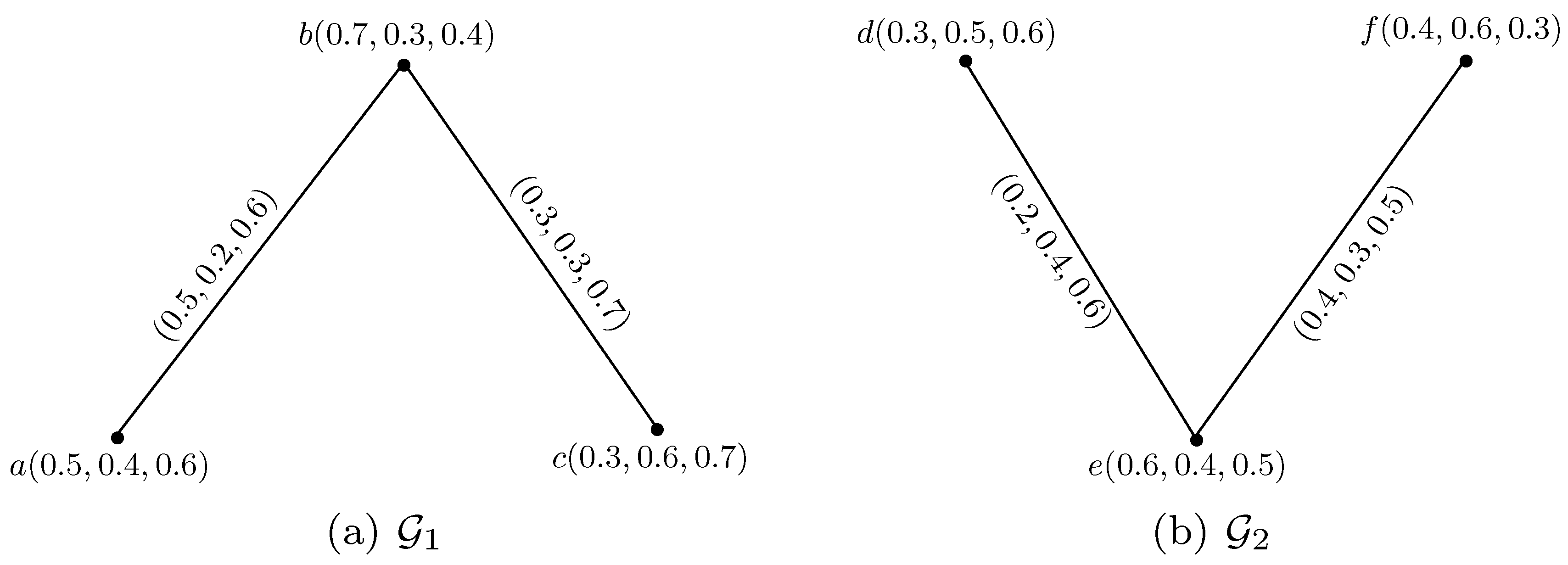
Consider two SFGs, ${\mathcal{G}}_1=(M_1,N_1)$ and ${\mathcal{G}}_2=(M_2,N_2)$, as shown in Figure 4. Then rejection of ${\mathcal{G}}_1$ and ${\mathcal{G}}_2$, i.e., ${\mathcal{G}}_1|{\mathcal{G}}_2$ is shown in Figure 5.

Proposition 2.

If ${\mathcal{G}}_1$ and ${\mathcal{G}}_2$ are SFGs, then ${\mathcal{G}}_1|{\mathcal{G}}_2$ is an SFG.

Proof. 

Let $a\in V_1$ and $a_2{b}_2\notin E_2$. Then we have

$$\begin{array}{cc}\hfill \left({\alpha }_{N_1}|{\alpha }_{N_2}\right)(a,a_2)(a,b_2)& =min\left({\alpha }_{M_1}\left(a\right),{\alpha }_{M_2}\left(a_2\right),{\alpha }_{M_2}\left(b_2\right)\right)\hfill \\ \hfill & =min\left(min\left({\alpha }_{M_1}\left(a\right),{\alpha }_{M_2}\left(a_2\right)\right),min\left({\alpha }_{M_1}\left(a\right),{\alpha }_{M_2}\left(b_2\right)\right)\right)\hfill \\ \hfill & =min\left(\left({\alpha }_{M_1}|{\alpha }_{M_2}\right)(a,a_2),\left({\alpha }_{M_1}|{\alpha }_{M_2}\right)(a,b_2)\right),\hfill \end{array}$$

$$\begin{array}{cc}\hfill \left({\gamma }_{N_1}|{\gamma }_{N_2}\right)(a,a_2)(a,b_2)& =min\left({\gamma }_{M_1}\left(a\right),{\gamma }_{M_2}\left(a_2\right),{\gamma }_{M_2}\left(b_2\right)\right)\hfill \\ \hfill & =min\left(min\left({\gamma }_{M_1}\left(a\right),{\gamma }_{M_2}\left(a_2\right)\right),min\left({\gamma }_{M_1}\left(a\right),{\gamma }_{M_2}\left(b_2\right)\right)\right)\hfill \\ \hfill & =min\left(\left({\gamma }_{M_1}|{\gamma }_{M_2}\right)(a,a_2),\left({\gamma }_{M_1}|{\gamma }_{M_2}\right)(a,b_2)\right),\hfill \end{array}$$

$$\begin{array}{cc}\hfill \left({\beta }_{N_1}|{\beta }_{N_2}\right)(a,a_2)(a,b_2)& =max\left({\beta }_{M_1}\left(a\right),{\beta }_{M_2}\left(a_2\right),{\beta }_{M_2}\left(b_2\right)\right)\hfill \\ \hfill & =max\left(max\left({\beta }_{M_1}\left(a\right),{\beta }_{M_2}\left(a_2\right)\right),max\left({\beta }_{M_1}\left(a\right),{\beta }_{M_2}\left(b_2\right)\right)\right)\hfill \\ \hfill & =max\left(\left({\beta }_{M_1}|{\beta }_{M_2}\right)(a,a_2),\left({\beta }_{M_1}|{\beta }_{M_2}\right)(a,b_2)\right).\hfill \end{array}$$

Let $c\in V_2$ and $a_1{b}_1\notin E_1$. Then we have

$$\begin{array}{cc}\hfill \left({\alpha }_{N_1}|{\alpha }_{N_2}\right)(a_1,c)(b_1,c)& =min\left({\alpha }_{M_1}\left(a_1\right),{\alpha }_{M_1}\left(b_1\right),{\alpha }_{M_2}\left(c\right)\right)\hfill \\ \hfill & =min\left(min\left({\alpha }_{M_1}\left(a_1\right),{\alpha }_{M_2}\left(c\right)\right),min\left({\alpha }_{M_1}\left(b_1\right),{\alpha }_{M_2}\left(c\right)\right)\right)\hfill \\ \hfill & =min\left(\left({\alpha }_{M_1}|{\alpha }_{M_2}\right)(a_1,c),\left({\alpha }_{M_1}|{\alpha }_{M_2}\right)(b_1,c)\right),\hfill \end{array}$$

$$\begin{array}{cc}\hfill \left({\gamma }_{N_1}|{\gamma }_{N_2}\right)(a_1,c)(b_1,c)& =min\left({\gamma }_{M_1}\left(a_1\right),{\gamma }_{M_1}\left(b_1\right),{\gamma }_{M_2}\left(c\right)\right)\hfill \\ \hfill & =min\left(min\left({\gamma }_{M_1}\left(a_1\right),{\gamma }_{M_2}\left(c\right)\right),min\left({\gamma }_{M_1}\left(b_1\right),{\gamma }_{M_2}\left(c\right)\right)\right)\hfill \\ \hfill & =min\left(\left({\gamma }_{M_1}|{\gamma }_{M_2}\right)(a_1,c),\left({\gamma }_{M_1}|{\gamma }_{M_2}\right)(b_1,c)\right),\hfill \end{array}$$

$$\begin{array}{cc}\hfill \left({\beta }_{N_1}|{\beta }_{N_2}\right)(a_1,c)(b_1,c)& =max\left({\beta }_{M_1}\left(a_1\right),{\beta }_{M_1}\left(b_1\right),{\beta }_{M_2}\left(c\right)\right)\hfill \\ \hfill & =max\left(max\left({\beta }_{M_1}\left(a_1\right),{\beta }_{M_2}\left(c\right)\right),max\left({\beta }_{M_1}\left(b_1\right),{\beta }_{M_2}\left(c\right)\right)\right)\hfill \\ \hfill & =max\left(\left({\beta }_{M_1}|{\beta }_{M_2}\right)(a_1,c),\left({\beta }_{M_1}|{\beta }_{M_2}\right)(b_1,c)\right).\hfill \end{array}$$

Let $a_1{b}_1\notin E_1,a_2{b}_2\notin E_2$. Then we have

$$\begin{array}{cc}\hfill \left({\alpha }_{N_1}|{\alpha }_{N_2}\right)(a_1,a_2)(b_1,b_2)& =min\left({\alpha }_{M_1}\left(a_1\right),{\alpha }_{M_1}\left(b_1\right),{\alpha }_{M_2}\left(a_2\right),{\alpha }_{M_2}\left(b_2\right)\right)\hfill \\ \hfill & =min\left(min\left({\alpha }_{M_1}\left(a_1\right),{\alpha }_{M_2}\left(a_2\right)\right),min\left({\alpha }_{M_1}\left(b_1\right),{\alpha }_{M_2}\left(b_2\right)\right)\right)\hfill \\ \hfill & =min\left(\left({\alpha }_{M_1}|{\alpha }_{M_2}\right)(a_1,a_2),\left({\alpha }_{M_1}|{\alpha }_{M_2}\right)(b_1,b_2)\right),\hfill \end{array}$$

$$\begin{array}{cc}\hfill \left({\gamma }_{N_1}|{\gamma }_{N_2}\right)(a_1,a_2)(b_1,b_2)& =min\left({\gamma }_{M_1}\left(a_1\right),{\gamma }_{M_1}\left(b_1\right),{\gamma }_{M_2}\left(a_2\right),{\gamma }_{M_2}\left(b_2\right)\right)\hfill \\ \hfill & =min\left(min\left({\gamma }_{M_1}\left(a_1\right),{\gamma }_{M_2}\left(a_2\right)\right),min\left({\gamma }_{M_1}\left(b_1\right),{\gamma }_{M_2}\left(b_2\right)\right)\right)\hfill \\ \hfill & =min\left(\left({\gamma }_{M_1}|{\gamma }_{M_2}\right)(a_1,a_2),\left({\gamma }_{M_1}|{\gamma }_{M_2}\right)(b_1,b_2)\right),\hfill \end{array}$$

$$\begin{array}{cc}\hfill \left({\beta }_{N_1}|{\beta }_{N_2}\right)(a_1,a_2)(b_1,b_2)& =max\left({\beta }_{M_1}\left(a_1\right),{\beta }_{M_1}\left(b_1\right),{\beta }_{M_2}\left(a_2\right),{\beta }_{M_2}\left(b_2\right)\right)\hfill \\ \hfill & =max\left(max\left({\beta }_{M_1}\left(a_1\right),{\beta }_{M_2}\left(a_2\right)\right),max\left({\beta }_{M_1}\left(b_1\right),{\beta }_{M_2}\left(b_2\right)\right)\right)\hfill \\ \hfill & =max\left(\left({\beta }_{M_1}|{\beta }_{M_2}\right)(a_1,a_2),\left({\beta }_{M_1}|{\beta }_{M_2}\right)(b_1,b_2)\right).\hfill \end{array}$$

Hence, ${\mathcal{G}}_1|{\mathcal{G}}_2$ is an SFG. □

Definition 9.

Let ${\mathcal{G}}_1=(M_1,N_1)$ and ${\mathcal{G}}_2=(M_2,N_2)$ be two SFGs. Then for any vertex, $(a_1,a_2)\in V_1\times V_2,$

$$\begin{array}{cc}\hfill {\left(d_{\alpha }\right)}_{{\mathcal{G}}_1|{\mathcal{G}}_2}(a_1,a_2)& =\sum _{(a_1,a_2)(b_1,b_2)\in E_1|E_2}\left({\alpha }_{N_1}|{\alpha }_{N_2}\right)(a_1,a_2)(b_1,b_2)\hfill \\ \hfill & =\sum _{a_1=b_1,a_2{b}_2\notin E_2}min\{{\alpha }_{M_1}\left(a_1\right),{\alpha }_{M_2}\left(a_2\right),{\alpha }_{M_2}\left(b_2\right)\}+\sum _{a_2=b_2,a_1{b}_1\notin E_1}min\{{\alpha }_{M_2}\left(a_2\right),{\alpha }_{M_1}\left(a_1\right),{\alpha }_{M_1}\left(b_1\right)\}\hfill \\ \hfill & +\sum _{a_1{b}_1\notin E_1,a_2{b}_2\notin E_2}min\{{\alpha }_{M_1}\left(a_1\right),{\alpha }_{M_1}\left(b_1\right),{\alpha }_{M_2}\left(a_2\right),{\alpha }_{M_2}\left(b_2\right)\},\hfill \end{array}$$

$$\begin{array}{cc}\hfill {\left(d_{\gamma }\right)}_{{\mathcal{G}}_1|{\mathcal{G}}_2}(a_1,a_2)& =\sum _{(a_1,a_2)(b_1,b_2)\in E_1|E_2}\left({\gamma }_{N_1}|{\gamma }_{N_2}\right)(a_1,a_2)(b_1,b_2)\hfill \\ \hfill & =\sum _{a_1=b_1,a_2{b}_2\notin E_2}min\{{\gamma }_{M_1}\left(a_1\right),{\gamma }_{M_2}\left(a_2\right),{\gamma }_{M_2}\left(b_2\right)\}+\sum _{a_2=b_2,a_1{b}_1\notin E_1}min\{{\gamma }_{M_2}\left(a_2\right),{\gamma }_{M_1}\left(a_1\right),{\gamma }_{M_1}\left(b_1\right)\}\hfill \\ \hfill & +\sum _{a_1{b}_1\notin E_1,a_2{b}_2\notin E_2}min\{{\gamma }_{M_1}\left(a_1\right),{\gamma }_{M_1}\left(b_1\right),{\gamma }_{M_2}\left(a_2\right),{\gamma }_{M_2}\left(b_2\right)\},\hfill \end{array}$$

$$\begin{array}{cc}\hfill {\left(d_{\beta }\right)}_{{\mathcal{G}}_1|{\mathcal{G}}_2}(a_1,a_2)& =\sum _{(a_1,a_2)(b_1,b_2)\in E_1|E_2}\left({\beta }_{N_1}|{\beta }_{N_2}\right)(a_1,a_2)(b_1,b_2)\hfill \\ \hfill & =\sum _{a_1=b_1,a_2{b}_2\notin E_2}max\{{\beta }_{M_1}\left(a_1\right),{\beta }_{M_2}\left(a_2\right),{\beta }_{M_2}\left(b_2\right)\}+\sum _{a_2=b_2,a_1{b}_1\notin E_1}max\{{\beta }_{M_2}\left(a_2\right),{\beta }_{M_1}\left(a_1\right),{\beta }_{M_1}\left(b_1\right)\}\hfill \\ \hfill & +\sum _{a_1{b}_1\notin E_1,a_2{b}_2\notin E_2}max\{{\beta }_{M_1}\left(a_1\right),{\beta }_{M_1}\left(b_1\right),{\beta }_{M_2}\left(a_2\right),{\beta }_{M_2}\left(b_2\right)\}.\hfill \end{array}$$

Definition 10.

Let ${\mathcal{G}}_1=(M_1,N_1)$ and ${\mathcal{G}}_2=(M_2,N_2)$ be two SFGs. Then for any vertex, $(a_1,a_2)\in V_1\times V_2,$

$$\begin{array}{cc}\hfill {\left(t{d}_{\alpha }\right)}_{{\mathcal{G}}_1|{\mathcal{G}}_2}(a_1,a_2)& =\sum _{(a_1,a_2)(b_1,b_2)\in E_1|E_2}\left({\alpha }_{N_1}|{\alpha }_{N_2}\right)(a_1,a_2)(b_1,b_2)+\left({\alpha }_{M_1}|{\alpha }_{M_2}\right)(a_1,a_2)\hfill \\ \hfill & =\sum _{a_1=b_1,a_2{b}_2\notin E_2}min\{{\alpha }_{M_1}\left(a_1\right),{\alpha }_{M_2}\left(a_2\right),{\alpha }_{M_2}\left(b_2\right)\}+\sum _{a_2=b_2,a_1{b}_1\notin E_1}min\{{\alpha }_{M_2}\left(a_2\right),{\alpha }_{M_1}\left(a_1\right),{\alpha }_{M_1}\left(b_1\right)\}\hfill \\ \hfill & +\sum _{a_1{b}_1\notin E_1,a_2{b}_2\notin E_2}min\{{\alpha }_{M_1}\left(a_1\right),{\alpha }_{M_1}\left(b_1\right),{\alpha }_{M_2}\left(a_2\right),{\alpha }_{M_2}\left(b_2\right)\}+min\{{\alpha }_{M_1}\left(a_1\right),{\alpha }_{M_2}\left(a_2\right)\},\hfill \end{array}$$

$$\begin{array}{cc}\hfill {\left(t{d}_{\gamma }\right)}_{{\mathcal{G}}_1|{\mathcal{G}}_2}(a_1,a_2)& =\sum _{(a_1,a_2)(b_1,b_2)\in E_1|E_2}\left({\gamma }_{N_1}|{\gamma }_{N_2}\right)(a_1,a_2)(b_1,b_2)+\left({\gamma }_{M_1}|{\gamma }_{M_2}\right)(a_1,a_2)\hfill \\ \hfill & =\sum _{a_1=b_1,a_2{b}_2\notin E_2}min\{{\gamma }_{M_1}\left(a_1\right),{\gamma }_{M_2}\left(a_2\right),{\gamma }_{M_2}\left(b_2\right)\}+\sum _{a_2=b_2,a_1{b}_1\notin E_1}min\{{\gamma }_{M_2}\left(a_2\right),{\gamma }_{M_1}\left(a_1\right),{\gamma }_{M_1}\left(b_1\right)\}\hfill \\ \hfill & +\sum _{a_1{b}_1\notin E_1,a_2{b}_2\notin E_2}min\{{\gamma }_{M_1}\left(a_1\right),{\gamma }_{M_1}\left(b_1\right),{\gamma }_{M_2}\left(a_2\right),{\gamma }_{M_2}\left(b_2\right)\}+min\{{\gamma }_{M_1}\left(a_1\right),{\gamma }_{M_2}\left(a_2\right)\},\hfill \end{array}$$

$$\begin{array}{cc}\hfill {\left(t{d}_{\beta }\right)}_{{\mathcal{G}}_1|{\mathcal{G}}_2}(a_1,a_2)& =\sum _{(a_1,a_2)(b_1,b_2)\in E_1|E_2}\left({\beta }_{N_1}|{\beta }_{N_2}\right)(a_1,a_2)(b_1,b_2)+\left({\beta }_{M_1}|{\beta }_{M_2}\right)(a_1,a_2)\hfill \\ \hfill & =\sum _{a_1=b_1,a_2{b}_2\notin E_2}max\{{\beta }_{M_1}\left(a_1\right),{\beta }_{M_2}\left(a_2\right),{\beta }_{M_2}\left(b_2\right)\}+\sum _{a_2=b_2,a_1{b}_1\notin E_1}max\{{\beta }_{M_2}\left(a_2\right),{\beta }_{M_1}\left(a_1\right),{\beta }_{M_1}\left(b_1\right)\}\hfill \\ \hfill & +\sum _{a_1{b}_1\notin E_1,a_2{b}_2\notin E_2}max\{{\beta }_{M_1}\left(a_1\right),{\beta }_{M_1}\left(b_1\right),{\beta }_{M_2}\left(a_2\right),{\beta }_{M_2}\left(b_2\right)\}+max\{{\beta }_{M_1}\left(a_1\right),{\beta }_{M_2}\left(a_2\right)\}.\hfill \end{array}$$

3. Irregularity in Spherical Fuzzy Graphs

The concept of irregularity has been explored by many researchers on fuzzy graphs and several of its extensions. We now define irregularity for spherical fuzzy graphs.

Definition 11.

An SFG $\mathcal{G}=(M,N)$ is said to be an irregular-spherical fuzzy graph (I-SFG) if ∃ a vertex which is adjacent to vertices with different degrees.

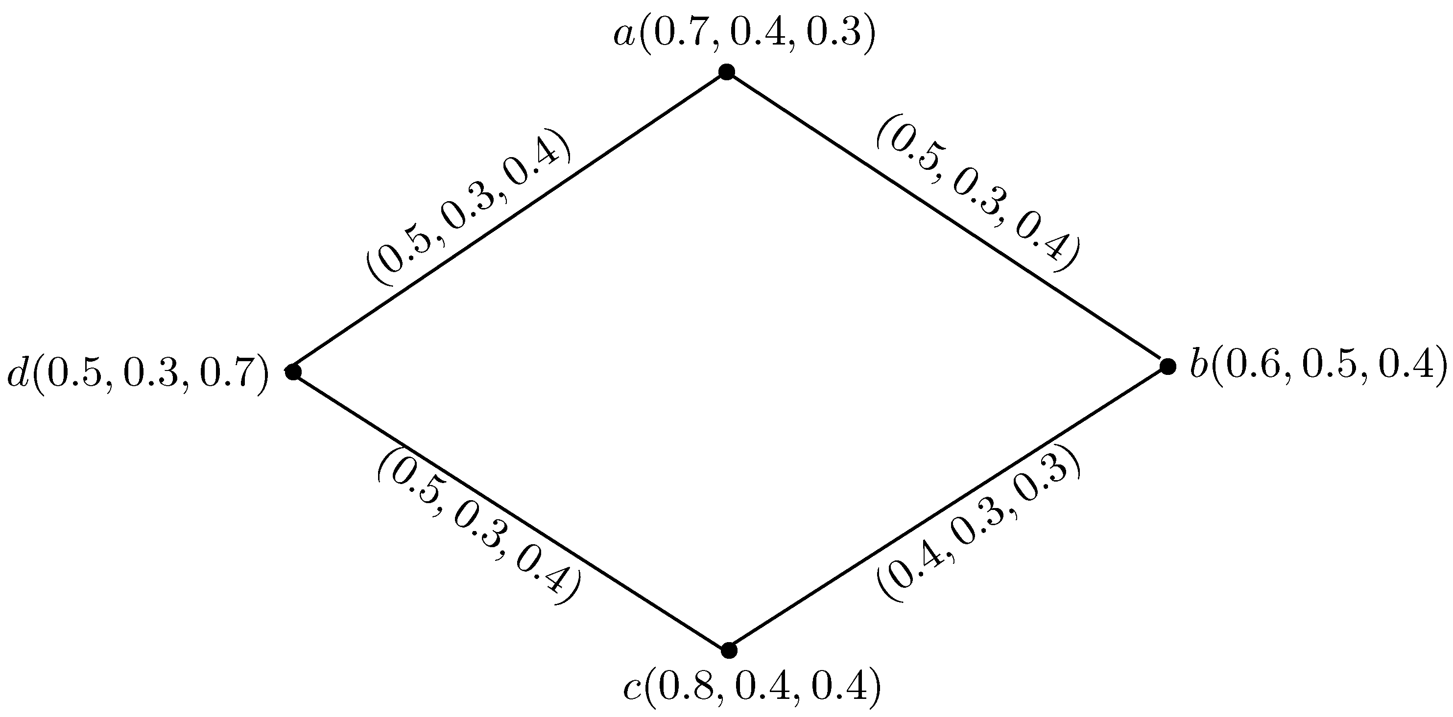
Example 4.

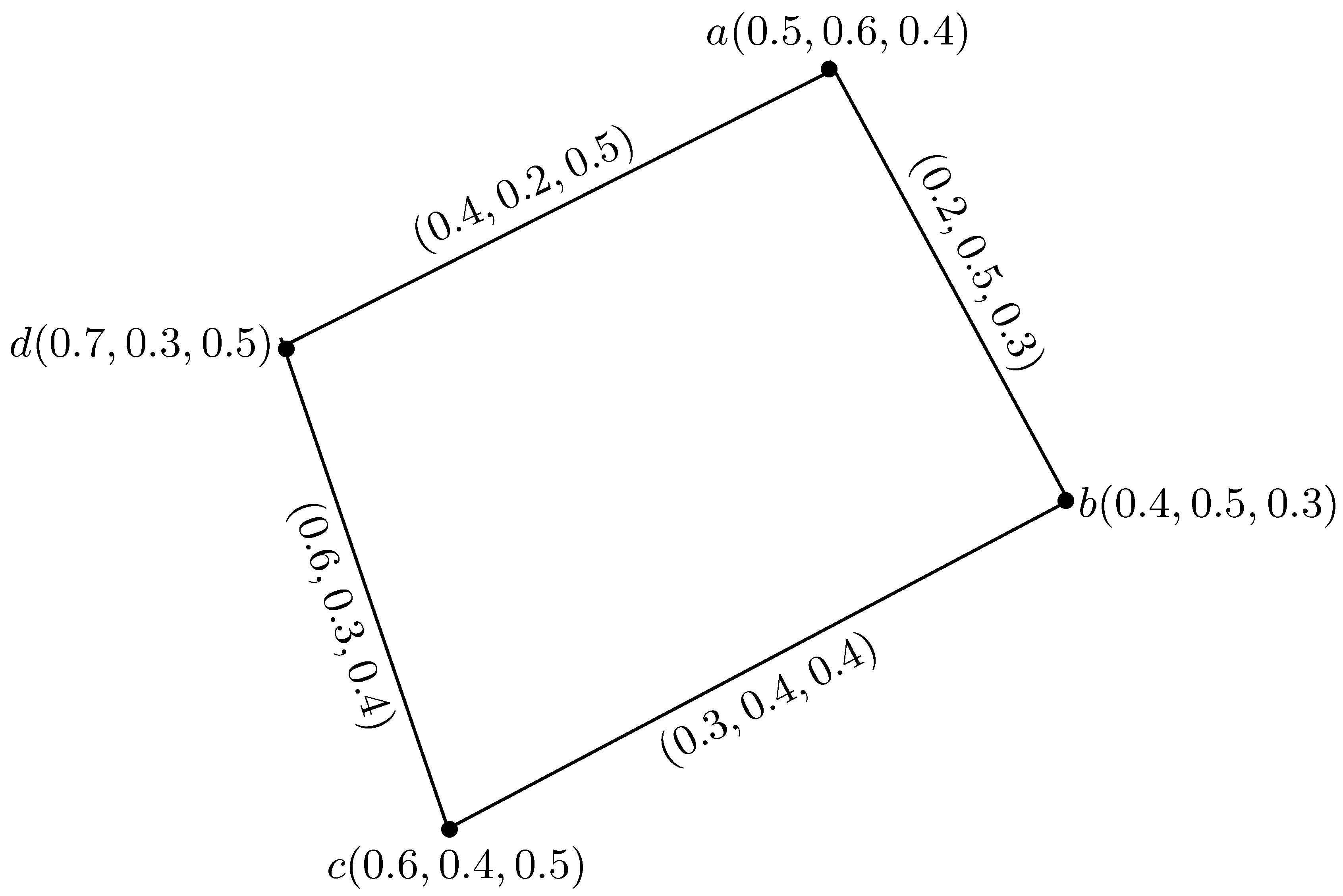
Consider an SFG $\mathcal{G}=(M,N)$ on a crisp graph $G^{*}=(V,E)$, such that $V=\{a,b,c,d\}$ and $E=\{ab,ad,bc,cd\},$ as shown in Figure 6.

By direct computation, we have $d_{\mathcal{G}}\left(a\right)=(0.6,0.4,0.1),d_{\mathcal{G}}\left(b\right)=(0.5,0.3,0.9),d_{\mathcal{G}}\left(c\right)=(0.5,0.3,0.9)$ and $d_{\mathcal{G}}\left(d\right)=(0.6,0.4,0.1).$ From this, we can see that a is adjacent to vertices of different degrees. So, $\mathcal{G}$ is an I-SFG.

Definition 12.

An SFG $\mathcal{G}=(M,N)$ is said to be a totally irregular-spherical fuzzy graph (TI-SFG) if ∃ a vertex which is adjacent to vertices with different total degrees.

Example 5.

Consider an SFG $\mathcal{G}=(M,N)$ on a crisp graph $G^{*}=(V,E)$ such that $V=\{a,b,c,d\}$ and $E=\{ab,ad,bc,cd\},$ as shown in Figure 7.

By direct computation, we have $t{d}_{\mathcal{G}}\left(a\right)=(1.7,1.0,1.1),t{d}_{\mathcal{G}}\left(b\right)=(1.5,1.1,1.1),t{d}_{\mathcal{G}}\left(c\right)=(1.7,1.0,1.1)$ and $t{d}_{\mathcal{G}}\left(d\right)=(1.5,0.9,1.1).$ From this, we can see that a is adjacent to vertices of different total degrees. So, $\mathcal{G}$ is a TI-SFG.

Definition 13.

An SFG $\mathcal{G}=(M,N)$ is said to be strongly I-SFG if every vertex has a different degree.

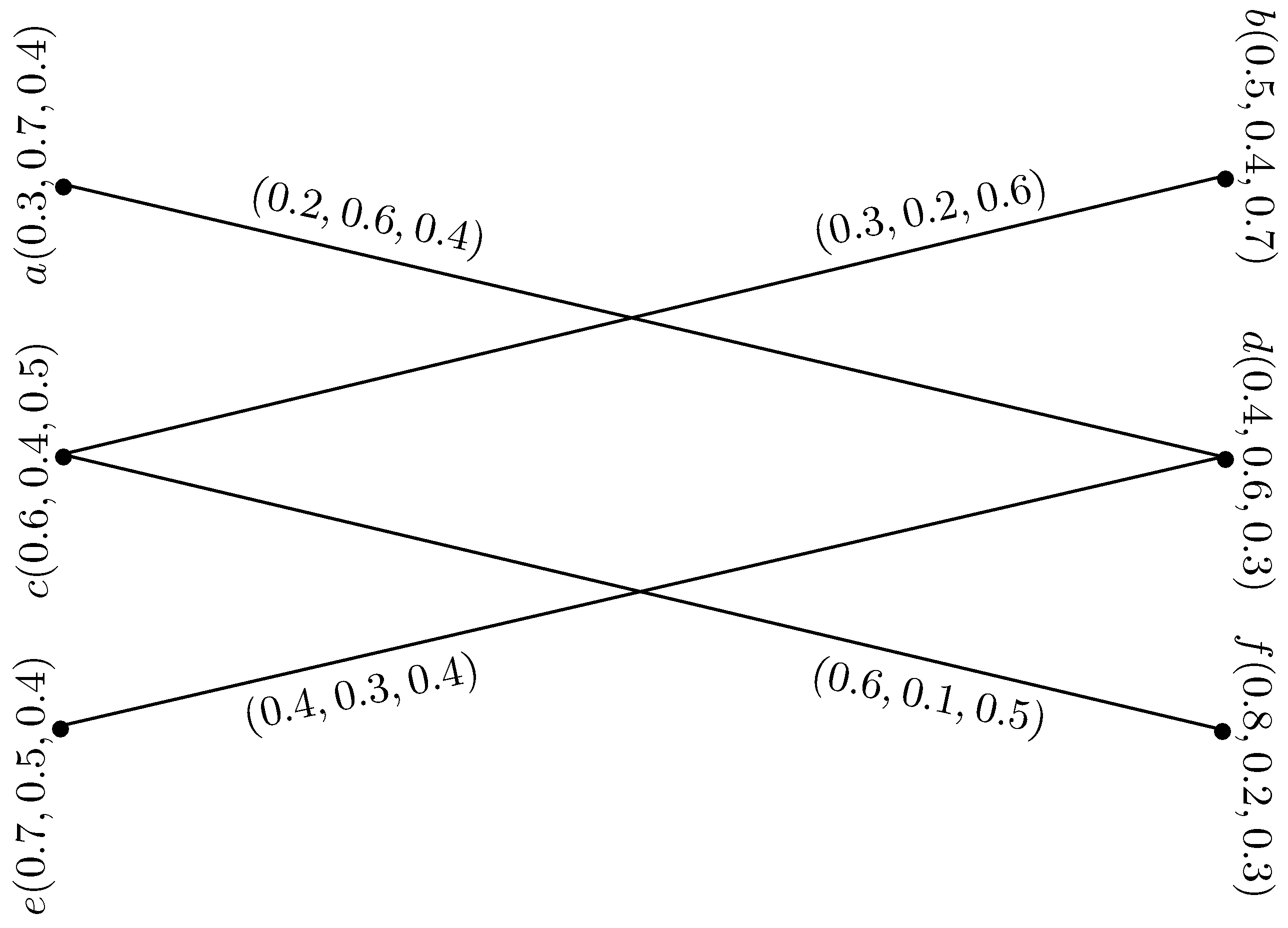
Example 6.

Consider an SFG $\mathcal{G}=(M,N)$ on a crisp graph $G^{*}=(V,E)$ such that $V=\{a,b,c,d,e,f\}$ and $E=\{ad,bc,de,cf\},$ as shown in Figure 8.

By direct computation, we have $d_{\mathcal{G}}\left(a\right)=(0.2,0.6,0.4),d_{\mathcal{G}}\left(b\right)=(0.3,0.2,0.6),d_{\mathcal{G}}\left(c\right)=(0.9,0.3,1.1),d_{\mathcal{G}}\left(d\right)=(0.6,0.9,0.8),d_{\mathcal{G}}\left(e\right)=(0.4,0.3,0.4)$, and $d_{\mathcal{G}}\left(f\right)=(0.6,0.1,0.5).$ From this, we can see that every vertex has a different degree. So, $\mathcal{G}$ is strongly I-SFG.

Definition 14.

An SFG $\mathcal{G}=(M,N)$ is said to be strongly TI-SFG if every vertex has a different total degree.

Example 7.

Consider an SFG $\mathcal{G}=(M,N)$ as shown in Figure 8. By direct computation, we have $t{d}_{\mathcal{G}}\left(a\right)=(0.5,1.3,0.8),t{d}_{\mathcal{G}}\left(b\right)=(0.8,0.6,1.3),t{d}_{\mathcal{G}}\left(c\right)=(1.5,0.7,1.6),t{d}_{\mathcal{G}}\left(d\right)=(1.0,1.5,1.1),t{d}_{\mathcal{G}}\left(e\right)=(1.1,0.8,0.8)$, and $t{d}_{\mathcal{G}}\left(f\right)=(1.4,0.3,0.8).$ From this, we can see that every vertex has a different total degree. So, G is strongly TI-SFG.

Definition 15.

An SFG $\mathcal{G}=(M,N)$ is said to be highly I-SFG if every vertex in $\mathcal{G}$ is adjacent to vertices of different degrees.

Example 8.

Consider an SFG $\mathcal{G}=(M,N)$ as shown in Figure 6. From this, we can see that every vertex is adjacent to vertices of different degrees. So, $\mathcal{G}$ is highly I-SFG.

Definition 16.

An SFG $\mathcal{G}=(M,N)$ is said to be highly TI-SFG if every vertex in $\mathcal{G}$ is adjacent to vertices of different total degrees.

Example 9.

Consider an SFG $\mathcal{G}=(M,N)$ on a crisp graph $G^{*}=(V,E)$ such that $V=\{a,b,c,d\}$ and $E=\{ab,ad,bc,cd\},$ as shown in Figure 9.

By direct computation, we have $t{d}_{\mathcal{G}}\left(a\right)=(1.1,0.9,1.4),t{d}_{\mathcal{G}}\left(b\right)=(1.0,1.1,1.5),t{d}_{\mathcal{G}}\left(c\right)=(1.2,0.8,1.7)$, and $t{d}_{\mathcal{G}}\left(d\right)=(0.9,0.9,1.7).$ From this, we can see that every vertex is adjacent to vertices of different degrees. So, $\mathcal{G}$ is a highly TI-SFG.

Definition 17.

The degree and the total degree of an edge $ab$ of a SFG $\mathcal{G}$ are denoted by $d_{\mathcal{G}}\left(ab\right)=(d_{\alpha }\left(ab\right),d_{\gamma }\left(ab\right),d_{\beta }\left(ab\right))$, and $t{d}_{\mathcal{G}}\left(ab\right)=(t{d}_{\alpha }\left(ab\right),t{d}_{\gamma }\left(ab\right),t{d}_{\beta }\left(ab\right))$, respectively, and are defined as

$$\begin{array}{cc}\hfill d_{\mathcal{G}}\left(ab\right)& =d_{\mathcal{G}}\left(a\right)+d_{\mathcal{G}}\left(b\right)-2({\alpha }_Y\left(ab\right),{\gamma }_Y\left(ab\right),{\beta }_Y\left(ab\right)),\hfill \\ \hfill t{d}_{\mathcal{G}}\left(ab\right)& =d_{\mathcal{G}}\left(ab\right)+({\alpha }_Y\left(ab\right),{\gamma }_Y\left(ab\right),{\beta }_Y\left(ab\right)).\hfill \end{array}$$

Example 10.

Consider an SFG $\mathcal{G}=(M,N)$ on a crisp graph $G^{*}=(V,E)$ such that $V=\{a,b,c,d\}$ and $E=\{ab,bc,cd\},$ as shown in Figure 10.

By direct computation, we have $d_{\mathcal{G}}\left(a\right)=(0.3,0.4,0.5),d_{\mathcal{G}}\left(b\right)=(0.5,0.9,0.9),d_{\mathcal{G}}\left(c\right)=(0.5,0.7,0.8)$, and$d_{\mathcal{G}}\left(d\right)=(0.3,0.2,0.4).$

• The degree of every edge is given as:

  $$\begin{array}{cc}\hfill d_{\mathcal{G}}\left(ab\right)& =d_{\mathcal{G}}\left(a\right)+d_{\mathcal{G}}\left(b\right)-2({\alpha }_Y\left(ab\right),{\gamma }_Y\left(ab\right),{\beta }_Y\left(ab\right)),\hfill \\ \hfill & =(0.3,0.4,0.5)+(0.5,0.9,0.9)-2(0.3,0.4,0.5),\hfill \\ \hfill & =(0.2,0.5,0.4),\hfill \\ \hfill d_{\mathcal{G}}\left(bc\right)& =d_{\mathcal{G}}\left(b\right)+d_{\mathcal{G}}\left(c\right)-2({\alpha }_Y\left(bc\right),{\gamma }_Y\left(bc\right),{\beta }_Y\left(bc\right)),\hfill \\ \hfill & =(0.5,0.9,0.9)+(0.5,0.7,0.8)-2(0.2,0.5,0.4),\hfill \\ \hfill & =(0.6,0.6,0.9),\hfill \\ \hfill d_{\mathcal{G}}\left(cd\right)& =d_{\mathcal{G}}\left(c\right)+d_{\mathcal{G}}\left(d\right)-2({\alpha }_Y\left(cd\right),{\gamma }_Y\left(cd\right),{\beta }_Y\left(cd\right)),\hfill \\ \hfill & =(0.5,0.7,0.8)+(0.3,0.2,0.4)-2(0.3,0.2,0.4),\hfill \\ \hfill & =(0.2,0.5,0.4).\hfill \end{array}$$
• The total degree of every edge is given as:

  $$\begin{array}{cc}\hfill t{d}_{\mathcal{G}}\left(ab\right)& =d_{\mathcal{G}}\left(ab\right)+({\alpha }_Y\left(ab\right),{\gamma }_Y\left(ab\right),{\beta }_Y\left(ab\right)),\hfill \\ \hfill & =(0.2,0.5,0.4)+(0.3,0.4,0.5),\hfill \\ \hfill & =(0.5,0.9,0.9),\hfill \\ \hfill t{d}_{\mathcal{G}}\left(bc\right)& =d_{\mathcal{G}}\left(bc\right)+({\alpha }_Y\left(bc\right),{\gamma }_Y\left(bc\right),{\beta }_Y\left(bc\right)),\hfill \\ \hfill & =(0.6,0.6,0.9)+(0.2,0.5,0.4),\hfill \\ \hfill & =(0.8,1.1,1.3),\hfill \\ \hfill t{d}_{\mathcal{G}}\left(cd\right)& =d_{\mathcal{G}}\left(cd\right)+({\alpha }_Y\left(cd\right),{\gamma }_Y\left(cd\right),{\beta }_Y\left(cd\right)),\hfill \\ \hfill & =(0.2,0.5,0.4)+(0.3,0.2,0.4),\hfill \\ \hfill & =(0.5,0.7,0.8).\hfill \end{array}$$

Definition 18.

A connected SFG $\mathcal{G}=(M,N)$ is said to be a neighborly edge irregular-spherical fuzzy graph (EI-SFG), if every pair of adjacent edges in $\mathcal{G}$ has different degrees.

Example 11.

Consider the SFG $\mathcal{G}=(M,N)$, as shown in Figure 10. From this, we can see that every pair of adjacent edges in $\mathcal{G}$ has different degrees. So $\mathcal{G}$ is a neighborly EI-SFG.

Definition 19.

A connected SFG $\mathcal{G}=(M,N)$ is said to be a neighborly edge TI-SFG, if every pair of adjacent edges in $\mathcal{G}$ has different total degrees.

Example 12.

Consider the SFG $\mathcal{G}=(M,N)$, as shown in Figure 10. From this, we can see that every pair of adjacent edges in $\mathcal{G}$ has different total degrees. So, $\mathcal{G}$ is a neighborly edge TI-SFG.

Definition 20.

An SFG $\mathcal{G}=(M,N)$ on a crisp graph $G^{*}$ is said to be a strongly EI-SFG if every edge in $\mathcal{G}$ has a different degree.

Example 13.

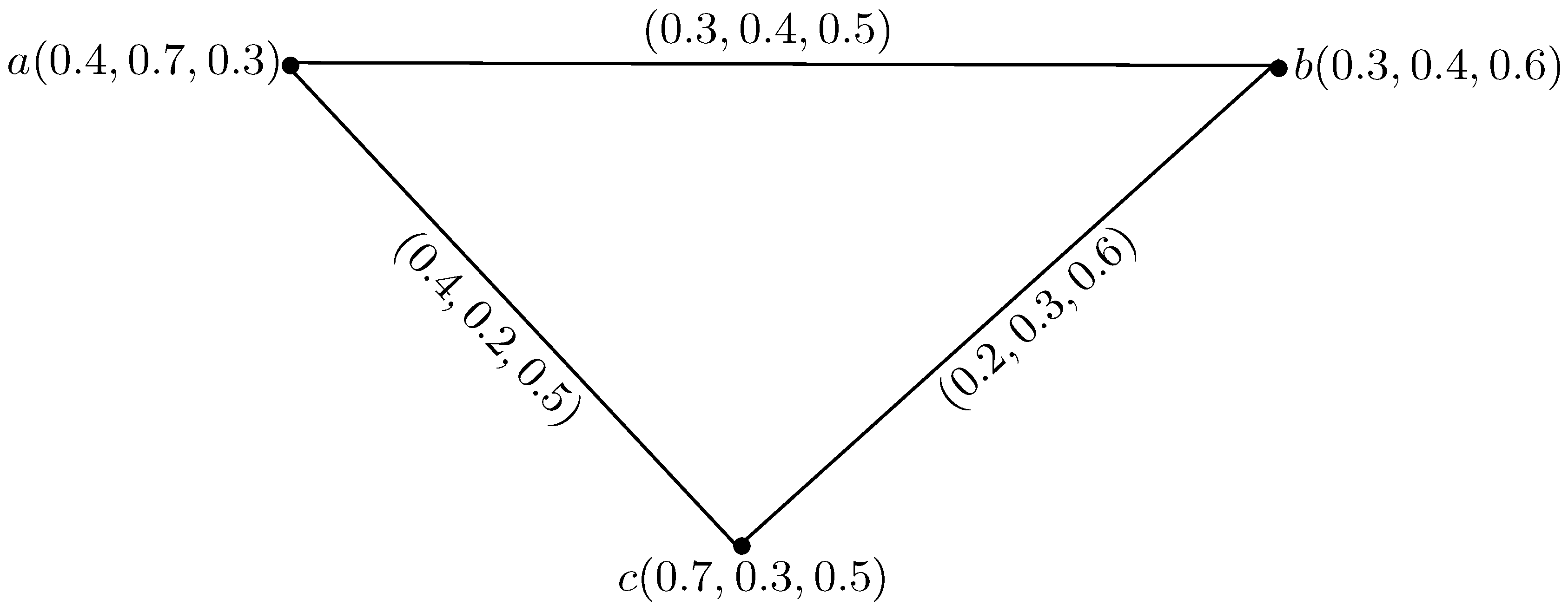
Consider an SFG $\mathcal{G}=(M,N)$ on a crisp graph $G^{*}=(V,E)$, such that $V=\{a,b,c\}$ and $E=\{ab,bc,cd\},$ as shown in Figure 11.

By direct computation, we have $d_{\mathcal{G}}\left(a\right)=(0.7,0.6,1.0),d_{\mathcal{G}}\left(b\right)=(0.5,0.7,1.1)$ and $d_{\mathcal{G}}\left(c\right)=(0.6,0.5,1.1).$

• The degree of every edge is given as:

  $$\begin{array}{cc}\hfill d_{\mathcal{G}}\left(ab\right)& =d_{\mathcal{G}}\left(a\right)+d_{\mathcal{G}}\left(b\right)-2({\alpha }_Y\left(ab\right),{\gamma }_Y\left(ab\right),{\beta }_Y\left(ab\right)),\hfill \\ \hfill & =(0.7,0.6,1.0)+(0.5,0.7,1.1)-2(0.3,0.4,0.5),\hfill \\ \hfill & =(0.6,0.5,1.1),\hfill \\ \hfill d_{\mathcal{G}}\left(bc\right)& =d_{\mathcal{G}}\left(b\right)+d_{\mathcal{G}}\left(c\right)-2({\alpha }_Y\left(bc\right),{\gamma }_Y\left(bc\right),{\beta }_Y\left(bc\right)),\hfill \\ \hfill & =(0.5,0.7,1.1)+(0.6,0.5,1.1)-2(0.2,0.3,0.6),\hfill \\ \hfill & =(0.7,0.6,1.0),\hfill \\ \hfill d_{\mathcal{G}}\left(ac\right)& =d_{\mathcal{G}}\left(a\right)+d_{\mathcal{G}}\left(c\right)-2({\alpha }_Y\left(ac\right),{\gamma }_Y\left(ac\right),{\beta }_Y\left(ac\right)),\hfill \\ \hfill & =(0.7,0.6,1.0)+(0.6,0.5,1.1)-2(0.4,0.2,0.5),\hfill \\ \hfill & =(0.5,0.7,1.1).\hfill \end{array}$$

Since every edge in $\mathcal{G}$ has a different degree, $\mathcal{G}$ is a strongly EI-SFG.

Definition 21.

An SFG $\mathcal{G}=(M,N)$ on a crisp graph $G^{*}$ is said to be a strongly edge TI-SFG, if every edge in $\mathcal{G}$ has a different total degree.

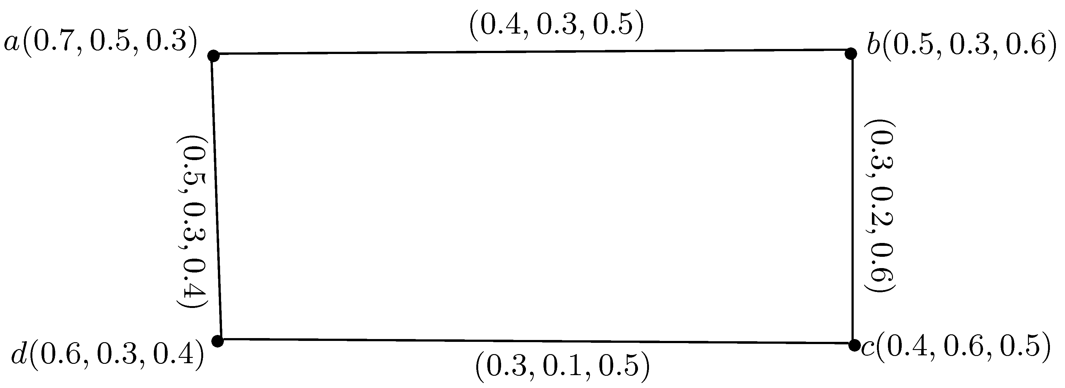
Example 14.

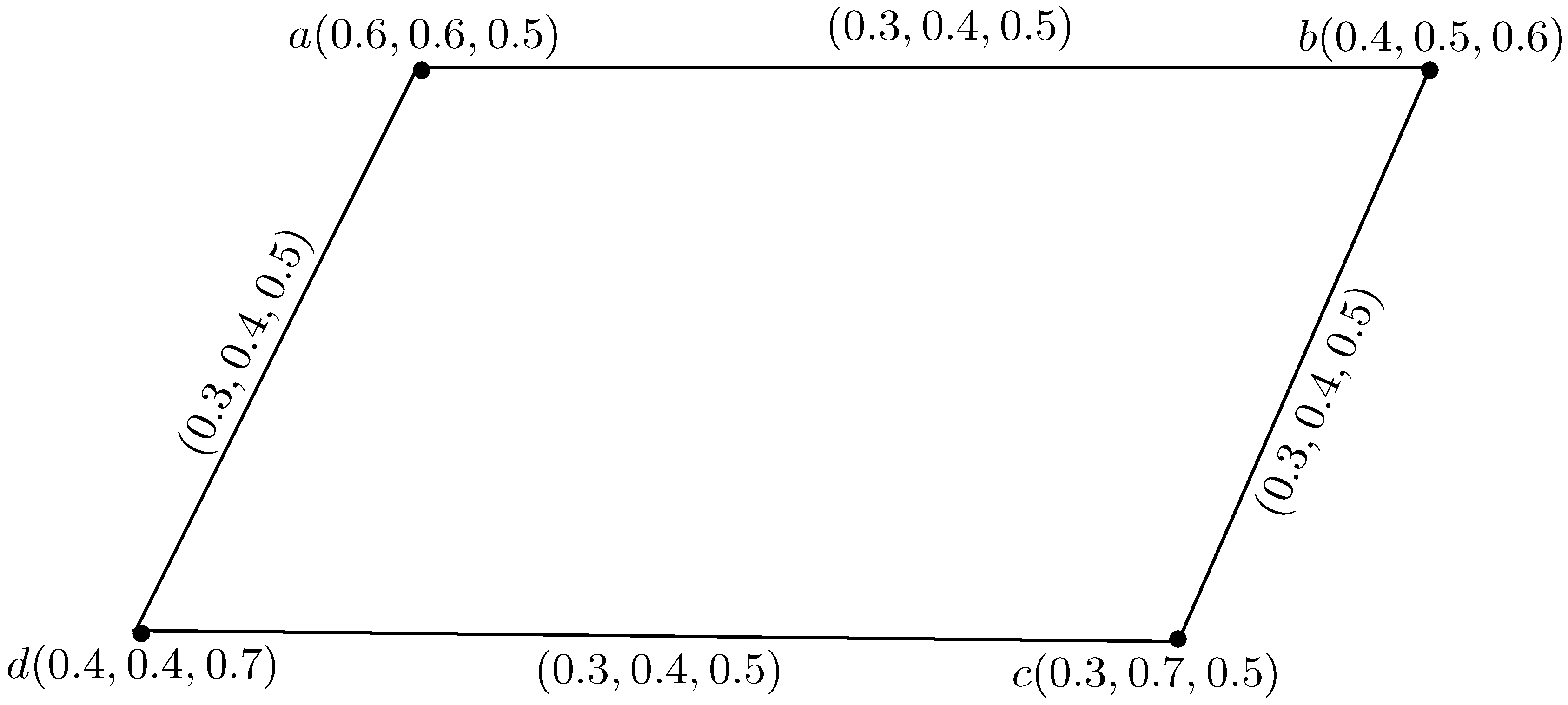
Consider an SFG $\mathcal{G}=(M,N)$ on a crisp graph $G^{*}=(V,E)$ such that $V=\{a,b,c,d\}$ and $E=\{ab,bc,cd,ad\},$ as shown in Figure 12.

By direct computation, we have $d_{\mathcal{G}}\left(a\right)=(0.9,0.6,0.9),d_{\mathcal{G}}\left(b\right)=(0.7,0.5,1.1),d_{\mathcal{G}}\left(c\right)=(0.6,0.3,1.1)$ and $d_{\mathcal{G}}\left(d\right)=(0.8,0.4,0.9).$

• The degree of every edge is given as:

  $$\begin{array}{cc}\hfill d_{\mathcal{G}}\left(ab\right)& =d_{\mathcal{G}}\left(a\right)+d_{\mathcal{G}}\left(b\right)-2({\alpha }_Y\left(ab\right),{\gamma }_Y\left(ab\right),{\beta }_Y\left(ab\right)),\hfill \\ \hfill & =(0.9,0.6,0.9)+(0.7,0.5,1.1)-2(0.4,0.3,0.5),\hfill \\ \hfill & =(0.8,0.5,1.0),\hfill \\ \hfill d_{\mathcal{G}}\left(bc\right)& =d_{\mathcal{G}}\left(b\right)+d_{\mathcal{G}}\left(c\right)-2({\alpha }_Y\left(bc\right),{\gamma }_Y\left(bc\right),{\beta }_Y\left(bc\right)),\hfill \\ \hfill & =(0.7,0.5,1.1)+(0.6,0.3,1.1)-2(0.3,0.2,0.6),\hfill \\ \hfill & =(0.7,0.4,1.0),\hfill \\ \hfill d_{\mathcal{G}}\left(cd\right)& =d_{\mathcal{G}}\left(c\right)+d_{\mathcal{G}}\left(d\right)-2({\alpha }_Y\left(cd\right),{\gamma }_Y\left(cd\right),{\beta }_Y\left(cd\right)),\hfill \\ \hfill & =(0.6,0.3,1.1)+(0.8,0.4,0.9)-2(0.3,0.1,0.5),\hfill \\ \hfill & =(0.8,0.5,1.0),\hfill \\ \hfill d_{\mathcal{G}}\left(ad\right)& =d_{\mathcal{G}}\left(a\right)+d_{\mathcal{G}}\left(d\right)-2({\alpha }_Y\left(ad\right),{\gamma }_Y\left(ad\right),{\beta }_Y\left(ad\right)),\hfill \\ \hfill & =(0.9,0.6,0.9)+(0.8,0.4,0.9)-2(0.5,0.3,0.4),\hfill \\ \hfill & =(0.7,0.4,1.0).\hfill \end{array}$$
• The total degree of every edge is given as:

  $$\begin{array}{cc}\hfill t{d}_{\mathcal{G}}\left(ab\right)& =d_{\mathcal{G}}\left(ab\right)+({\alpha }_Y\left(ab\right),{\gamma }_Y\left(ab\right),{\beta }_Y\left(ab\right)),\hfill \\ \hfill & =(0.8,0.5,1.0)+(0.4,0.3,0.5),\hfill \\ \hfill & =(1.2,0.8,1.5),\hfill \\ \hfill t{d}_{\mathcal{G}}\left(bc\right)& =d_{\mathcal{G}}\left(bc\right)+({\alpha }_Y\left(bc\right),{\gamma }_Y\left(bc\right),{\beta }_Y\left(bc\right)),\hfill \\ \hfill & =(0.7,0.4,1.0)+(0.3,0.2,0.6),\hfill \\ \hfill & =(1.0,0.6,1.6),\hfill \\ \hfill t{d}_{\mathcal{G}}\left(cd\right)& =d_{\mathcal{G}}\left(cd\right)+({\alpha }_Y\left(cd\right),{\gamma }_Y\left(cd\right),{\beta }_Y\left(cd\right)),\hfill \\ \hfill & =(0.8,0.5,1.0)+(0.3,0.1,0.5),\hfill \\ \hfill & =(1.1,0.6,1.5),\hfill \\ \hfill t{d}_{\mathcal{G}}\left(ad\right)& =d_{\mathcal{G}}\left(ad\right)+({\alpha }_Y\left(ad\right),{\gamma }_Y\left(ad\right),{\beta }_Y\left(ad\right)),\hfill \\ \hfill & =(0.7,0.4,1.0)+(0.5,0.3,0.4),\hfill \\ \hfill & =(1.2,0.7,1.4).\hfill \end{array}$$

Since every edge in $\mathcal{G}$ has a different total degree, $\mathcal{G}$ is a strongly edge TI-SFG.

Remark 1.

A strongly EI-SFG $\mathcal{G}$ may not be strongly edge TI-SFG.

Example 15.

Consider an SFG $\mathcal{G}=(M,N)$ on a crisp graph $G^{*}=(V,E)$ such that $V=\{a,b,c\}$ and $E=\{ab,bc,ac\},$ as shown in Figure 13.

By direct computation, we have $d_{\mathcal{G}}\left(a\right)=(0.7,0.5,1.1),d_{\mathcal{G}}\left(b\right)=(0.6,0.7,0.8)$ and $d_{\mathcal{G}}\left(c\right)=(0.5,0.6,0.9).$ The degree of every edge is $d_{\mathcal{G}}\left(ab\right)=(0.5,0.6,0.9),d_{\mathcal{G}}\left(bc\right)=(0.7,0.5,1.1)$, and $d_{\mathcal{G}}\left(ac\right)=(0.6,0.7,0.8).$ Since every edge in $\mathcal{G}$ has a different degree, $\mathcal{G}$ is a strongly EI-SFG. The total degree of every edge is $t{d}_{\mathcal{G}}\left(ab\right)=(1.4,0.6,1.1)=t{d}_{\mathcal{G}}\left(bc\right)=t{d}_{\mathcal{G}}\left(ac\right).$ Since all the edges of $\mathcal{G}$ have equal total degrees, $\mathcal{G}$ is not a strongly edge TI-SFG.

Remark 2.

A strongly edge TI-SFG $\mathcal{G}$ may not be a strongly EI-SFG.

Example 16.

Consider an SFG $\mathcal{G}=(M,N)$ on a crisp graph $G^{*}=(V,E)$ such that $V=\{a,b,c,d\}$ and $E=\{ab,bc,cd,ad\},$ as shown in Figure 14.

By direct computation, we have $d_{\mathcal{G}}\left(a\right)=(0.6,0.7,0.8),d_{\mathcal{G}}\left(b\right)=(0.5,0.9,0.7),d_{\mathcal{G}}\left(c\right)=(0.9,0.7,0.8)$, and $d_{\mathcal{G}}\left(d\right)=(1.0,0.5,0.9).$ The degree of every edge is $d_{\mathcal{G}}\left(ab\right)=(0.7,0.6,0.9),d_{\mathcal{G}}\left(bc\right)=(0.8,0.8,0.7),d_{\mathcal{G}}\left(cd\right)=(0.7,0.6,0.9)$, and $d_{\mathcal{G}}\left(ad\right)=(0.8,0.8,0.7).$ From this, we can see that $d_{\mathcal{G}}\left(ab\right)=d_{\mathcal{G}}\left(cd\right)$ and $d_{\mathcal{G}}\left(bc\right)=d_{\mathcal{G}}\left(ad\right).$ Thus, $\mathcal{G}$ is not a strongly EI-SFG. The total degree of every edge is $t{d}_{\mathcal{G}}\left(ab\right)=(0.9,1.1,1.2),t{d}_{\mathcal{G}}\left(bc\right)=(1.1,1.2,1.1),t{d}_{\mathcal{G}}\left(cd\right)=(1.3,0.9,1.3)$, and $t{d}_{\mathcal{G}}\left(ad\right)=(1.2,1.0,1.2).$ Since every edge in $\mathcal{G}$ have different total degree, $\mathcal{G}$ is a strongly edge TI-SFG.

Theorem 3.

If $\mathcal{G}=(M,N)$ is a strongly edge irregular connected SFG, where N is a constant function. Then $\mathcal{G}$ is a strongly edge TI-SFG.

Proof. 

Let $\mathcal{G}=(M,N)$ be a strongly edge irregular connected SFG. Consider N is a constant function. Then ${\alpha }_N\left(ab\right)=m_1,{\gamma }_N\left(ab\right)=m_2$ and ${\beta }_N\left(ab\right)=m_3,$ for all $ab\in E$, where $m_1,m_2$, and $m_3$ are constants. Consider two edges $ab$ and $cd$ in E. Since $\mathcal{G}$ is a strongly EI-SFG therefore $d_{\mathcal{G}}\left(ab\right)\ne d_{\mathcal{G}}\left(cd\right),$ where $ab$ and $cd$ are two edges in E. This shows that $d_{\mathcal{G}}\left(ab\right)+(m_1,m_2,m_3)\ne d_{\mathcal{G}}\left(cd\right)+(m_1,m_2,m_3).$ This implies that $d_{\mathcal{G}}\left(ab\right)+({\alpha }_N\left(ab\right),{\gamma }_N\left(ab\right),{\beta }_N\left(ab\right))\ne d_{\mathcal{G}}\left(cd\right)+({\alpha }_N\left(cd\right),{\gamma }_N\left(cd\right),{\beta }_N\left(cd\right)).$ Thus $t{d}_{\mathcal{G}}\left(ab\right)\ne t{d}_{\mathcal{G}}\left(cd\right),$ where $ab$ and $cd$ are two edges in E. Since the edges $ab$ and $cd,$ were taken to be arbitrary, this demonstrates every two edges in $\mathcal{G}$ have different total degrees. Hence $\mathcal{G}$ is a strongly edge TI-SFG. □

Theorem 4.

If $\mathcal{G}=(M,N)$ is a strongly edge totally irregular connected SFG, where N is a constant function. Then $\mathcal{G}$ is a strongly EI-SFG.

Proof. 

Let $\mathcal{G}=(M,N)$ be a strongly edge totally irregular connected SFG. Consider N is a constant function. Then ${\alpha }_N\left(ab\right)=m_1,{\gamma }_N\left(ab\right)=m_2$, and ${\beta }_N\left(ab\right)=m_3,$ for all $ab\in E,$ where $m_1,m_2$, and $m_3$ are constants. Consider the edges $ab$ and $cd$ in E. Since $\mathcal{G}$ is a strongly edge TI-SFG, therefore $t{d}_{\mathcal{G}}\left(ab\right)\ne t{d}_{\mathcal{G}}\left(cd\right),$ where $ab$ and $cd$ are edges in E. This shows that $d_{\mathcal{G}}\left(ab\right)+({\alpha }_N\left(ab\right),{\gamma }_N\left(ab\right),{\beta }_N\left(ab\right))\ne d_{\mathcal{G}}\left(cd\right)+({\alpha }_N\left(cd\right),{\gamma }_N\left(cd\right),{\beta }_N\left(cd\right)).$ This implies that $d_{\mathcal{G}}\left(ab\right)+(m_1,m_2,m_3)\ne d_{\mathcal{G}}\left(cd\right)+(m_1,m_2,m_3).$ Thus $d_{\mathcal{G}}\left(ab\right)\ne d_{\mathcal{G}}\left(cd\right),$ where $ab$ and $cd$ are edges in E. Since the edges $ab$ and $cd,$ were taken to be arbitrary this demonstrates every two edges in $\mathcal{G}$ have different degrees. Hence $\mathcal{G}$ is a strongly EI-SFG. □

Remark 3.

If $\mathcal{G}=(M,N)$ is both strongly EI-SFG and strongly edge TI-SFG, then it is not necessary that Y is a constant function.

Example 17.

Consider a SFG $\mathcal{G}=(M,N)$ on a crisp graph $G^{*}=(V,E)$ such that $V=\{a,b,c,d,e,f,g\}$ and $E=\{ab,bc,cd,de,ef,fg,ag\},$ as shown in Figure 15.

By direct computation, we have $d_{\mathcal{G}}\left(a\right)=(0.7,0.5,0.8),d_{\mathcal{G}}\left(b\right)=(0.5,0.8,0.6),d_{\mathcal{G}}\left(c\right)=(0.3,0.9,0.7),d_{\mathcal{G}}\left(d\right)=(0.4,0.8,0.6),d_{\mathcal{G}}\left(e\right)=(0.7,0.5,0.7),d_{\mathcal{G}}\left(f\right)=(0.9,0.3,0.9)$ and $d_{\mathcal{G}}\left(g\right)=(0.7,0.4,1.1).$ The degree of every edge is $d_{\mathcal{G}}\left(ab\right)=(0.4,0.7,1.0),d_{\mathcal{G}}\left(bc\right)=(0.6,0.7,0.5),d_{\mathcal{G}}\left(cd\right)=(0.3,0.9,0.7),d_{\mathcal{G}}\left(de\right)=(0.7,0.5,0.7),d_{\mathcal{G}}\left(ef\right)=(0.6,0.6,0.8),d_{\mathcal{G}}\left(fg\right)=(0.8,0.3,1.0)$ and $d_{\mathcal{G}}\left(ag\right)=(0.8,0.5,0.7).$ From this, we can see that every edge has a different degree. So, $\mathcal{G}$ is a strongly EI-SFG. The total degree of every edge is $t{d}_{\mathcal{G}}\left(ab\right)=(0.8,1.0,1.2),t{d}_{\mathcal{G}}\left(bc\right)=(0.7,1.2,0.9),t{d}_{\mathcal{G}}\left(cd\right)=(0.5,1.3,1.0),t{d}_{\mathcal{G}}\left(de\right)=(0.9,0.9,1.0),t{d}_{\mathcal{G}}\left(ef\right)=(1.1,0.7,1.2),t{d}_{\mathcal{G}}\left(fg\right)=(1.2,0.5,1.5)$ and $t{d}_{\mathcal{G}}\left(ag\right)=(1.1,0.7,1.3).$ Since every edge has a different total degree, so $\mathcal{G}$ is a strongly edge TI-SFG. From this, we can see that $\mathcal{G}=(M,N)$ is both strongly EI-SFG and strongly edge TI-SFG, but N is not a constant function.

Theorem 5.

Let $\mathcal{G}=(M,N)$ be a strongly EI-SFG. Then $\mathcal{G}$ is a neighborly EI-SFG.

Proof. 

Let $\mathcal{G}$ be a strongly EI-SFG. Then every edge in $\mathcal{G}$ has a different degree. This demonstrates that every two adjacent edges in $\mathcal{G}$ have different degrees. So, $\mathcal{G}$ is a neighborly EI-SFG. □

Theorem 6.

Let $\mathcal{G}=(M,N)$ be a strongly edge TI-SFG. Then $\mathcal{G}$ is a neighborly edge TI-SFG.

Proof. 

Let $\mathcal{G}$ be a strongly edge TI-SFG. Then every edge in $\mathcal{G}$ has a different total degree. This demonstrates that every two adjacent edges in $\mathcal{G}$ have different total degrees. So, $\mathcal{G}$ is a neighborly edge TI-SFG. □

Remark 4.

If $\mathcal{G}$ is a neighborly EI-SFG then it is not compulsory that $\mathcal{G}$ is a strongly EI-SFG.

Example 18.

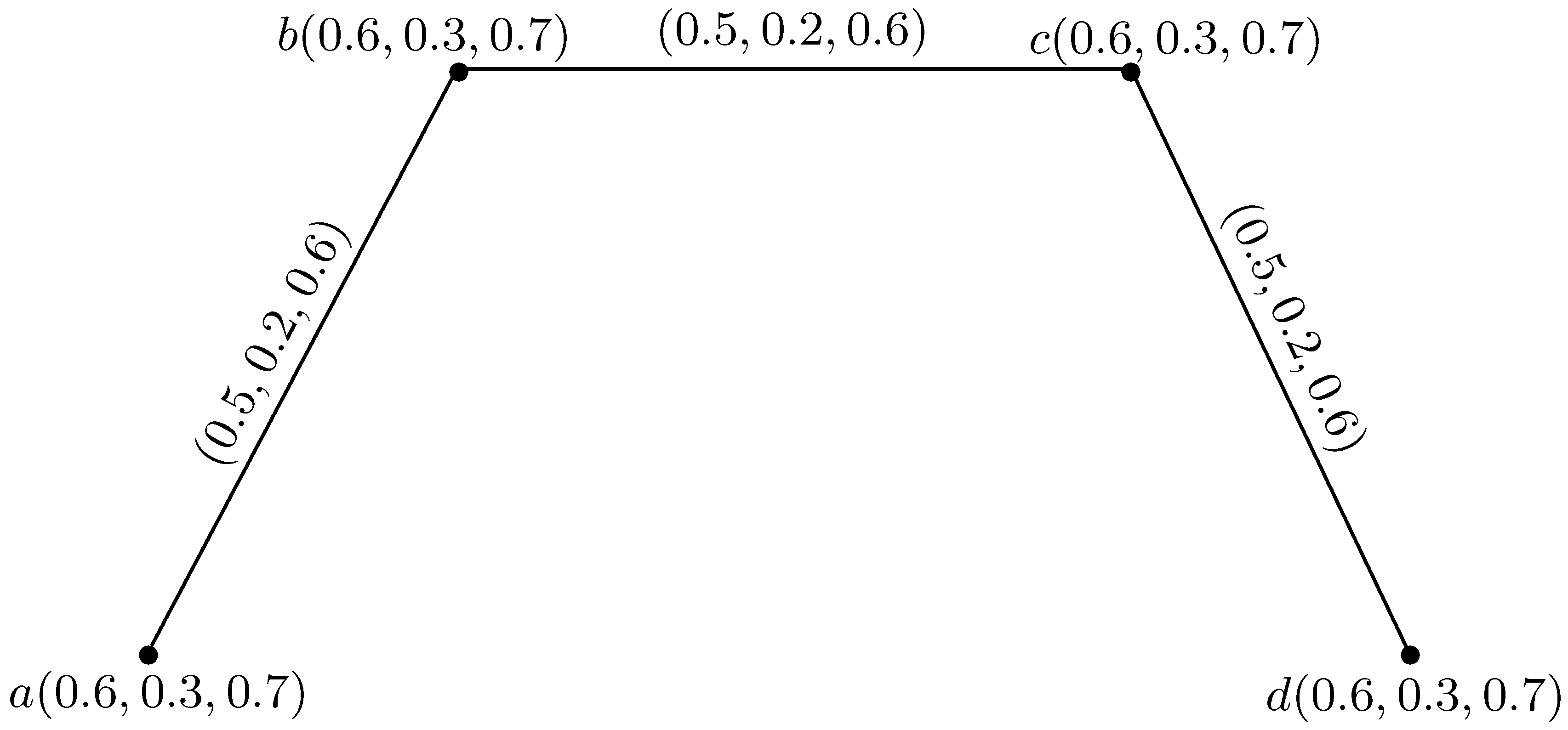
Consider a SFG $\mathcal{G}=(M,N)$ on a crisp graph $G^{*}=(V,E)$ such that $V=\{a,b,c,d\}$ and $E=\{ab,bc,cd\},$ as shown in Figure 16.

By direct computation, we have $d_{\mathcal{G}}\left(a\right)=(0.5,0.2,0.6),d_{\mathcal{G}}\left(b\right)=(1.0,0.4,1.2),d_{\mathcal{G}}\left(c\right)=(1.0,0.4,1.2)$ and $d_{\mathcal{G}}\left(d\right)=(0.5,0.2,0.6).$ The degree of every edge is $d_{\mathcal{G}}\left(ab\right)=(0.5,0.2,0.6),d_{\mathcal{G}}\left(bc\right)=(1.0,0.4,1.2)$ and $d_{\mathcal{G}}\left(cd\right)=(0.5,0.2,0.6).$ Since every two adjacent edges in $\mathcal{G}$ have different degrees, $i.e.,$$d_{\mathcal{G}}\left(ab\right)\ne d_{\mathcal{G}}\left(bc\right)$ and $d_{\mathcal{G}}\left(bc\right)\ne d_{\mathcal{G}}\left(cd\right).$ Therefore, $\mathcal{G}$ is a neighborly EI-SFG. From this, we can see that $d_{\mathcal{G}}\left(ab\right)=d_{\mathcal{G}}\left(cd\right).$ So, $\mathcal{G}$ is not a strongly EI-SFG.

Remark 5.

If $\mathcal{G}$ is a neighborly edge TI-SFG then it is not compulsory that $\mathcal{G}$ is a strongly edge TI-SFG.

Example 19.

Consider an SFG $\mathcal{G}=(M,N)$ as shown in Figure 16. The total degree of every edge is $t{d}_{\mathcal{G}}\left(ab\right)=(1.0,0.4,1.2),t{d}_{\mathcal{G}}\left(bc\right)=(1.5,0.6,1.8)$ and $t{d}_{\mathcal{G}}\left(cd\right)=(1.0,0.4,1.2).$ Since every two adjacent edges in $\mathcal{G}$ have different total degrees, i.e., $t{d}_{\mathcal{G}}\left(ab\right)\ne t{d}_{\mathcal{G}}\left(bc\right)$ and $t{d}_{\mathcal{G}}\left(bc\right)\ne t{d}_{\mathcal{G}}\left(cd\right).$ Therefore, $\mathcal{G}$ is a neighborly edge TI-SFG. From this, we can see that $t{d}_{\mathcal{G}}\left(ab\right)=t{d}_{\mathcal{G}}\left(cd\right).$ So, $\mathcal{G}$ is not a strongly edge TI-SFG.

Theorem 7.

Let $\mathcal{G}=(M,N)$ be a strongly edge irregular connected SFG, with N as constant function. Then $\mathcal{G}$ is an I-SFG.

Proof. 

Let $\mathcal{G}=(M,N)$ be a strongly edge irregular connected SFG, with N as constant function. Then ${\alpha }_N\left(ab\right)=m_1,{\gamma }_N\left(ab\right)=m_2$ and ${\beta }_N\left(ab\right)=m_3$ for every edge $ab\in E,$ where $m_1,m_2$, and $m_3$ are constants. Also, every edge in $\mathcal{G}$ has a different degree, so $\mathcal{G}$ is a strongly EI-SFG. Let $ab$ and $bc$ be any two adjacent edges in $\mathcal{G}$ such that $d_{\mathcal{G}}\left(ab\right)\ne d_{\mathcal{G}}\left(bc\right).$ This implies that $d_{\mathcal{G}}\left(a\right)+d_{\mathcal{G}}\left(b\right)-2({\alpha }_N\left(ab\right),{\gamma }_N\left(ab\right),{\beta }_N\left(ab\right))\ne d_{\mathcal{G}}\left(b\right)+d_{\mathcal{G}}\left(c\right)-2({\alpha }_N\left(bc\right),{\gamma }_N\left(bc\right),{\beta }_N\left(bc\right)).$ This implies that $d_{\mathcal{G}}\left(a\right)+d_{\mathcal{G}}\left(b\right)-2(m_1,m_2,m_3)\ne d_{\mathcal{G}}\left(b\right)+d_{\mathcal{G}}\left(c\right)-2(m_1,m_2,m_3).$ This shows that $d_{\mathcal{G}}\left(a\right)\ne d_{\mathcal{G}}\left(c\right).$ Thus ∃ a vertex b in $\mathcal{G}$ which is adjacent to the vertices with different degrees. This demonstrates that $\mathcal{G}$ is an I-SFG. □

Theorem 8.

Let $\mathcal{G}=(M,N)$ be a strongly edge totally irregular connected SFG, with N as constant function. Then $\mathcal{G}$ is an I-SFG.

Proof. 

Let $\mathcal{G}=(M,N)$ be a strongly edge totally irregular connected SFG, with N as constant function. Then ${\alpha }_N\left(ab\right)=m_1,{\gamma }_N\left(ab\right)=m_2$ and ${\beta }_N\left(ab\right)=m_3$ for every edge $ab\in E,$ where $m_1,m_2$, and $m_3$ are constants and every edge in $\mathcal{G}$ has a different total degree, so $\mathcal{G}$ is strongly edge TI-SFG. Let $ab$ and $bc$ be any two adjacent edges in $\mathcal{G}$ such that $t{d}_{\mathcal{G}}\left(ab\right)\ne t{d}_{\mathcal{G}}\left(bc\right).$ This implies that $d_{\mathcal{G}}\left(ab\right)+({\alpha }_N\left(ab\right),{\gamma }_N\left(ab\right),{\beta }_N\left(ab\right))\ne d_{\mathcal{G}}\left(bc\right)+({\alpha }_N\left(bc\right),{\gamma }_N\left(bc\right),{\beta }_N\left(bc\right)).$ This implies that $d_{\mathcal{G}}\left(a\right)+d_{\mathcal{G}}\left(b\right)-({\alpha }_N\left(ab\right),{\gamma }_N\left(ab\right),{\beta }_N\left(ab\right))\ne d_{\mathcal{G}}\left(b\right)+d_{\mathcal{G}}\left(c\right)-({\alpha }_N\left(bc\right),{\gamma }_N\left(bc\right),{\beta }_N\left(bc\right)).$ This implies that $d_{\mathcal{G}}\left(a\right)+d_{\mathcal{G}}\left(b\right)-2(m_1,m_2,m_3)\ne d_{\mathcal{G}}\left(b\right)+d_{\mathcal{G}}\left(c\right)-2(m_1,m_2,m_3).$ This shows that $d_{\mathcal{G}}\left(a\right)\ne d_{\mathcal{G}}\left(c\right).$ Thus ∃ a vertex b in $\mathcal{G}$ which is adjacent to the vertices with different degrees. This demonstrates that $\mathcal{G}$ is an I-SFG. □

Remark 6.

If $\mathcal{G}=(M,N)$ is an I-SFG, with N as a constant function. Then it is not compulsory that $\mathcal{G}$ is a strongly EI-SFG.

Example 20.

Consider a SFG $\mathcal{G}=(M,N)$ on a crisp graph $G^{*}=(V,E)$ such that $V=\{a,b,c,d\}$ and $E=\{ab,bc,bd,cd,ad\},$ as shown in Figure 17.

By direct computation, we have $d_{\mathcal{G}}\left(a\right)=(0.6,0.8,1.0),d_{\mathcal{G}}\left(b\right)=(0.9,1.2,1.5),d_{\mathcal{G}}\left(c\right)=(0.6,0.8,1.0)$ and $d_{\mathcal{G}}\left(d\right)=(0.9,1.2,1.5).$ The degree of every edge is $d_{\mathcal{G}}\left(ab\right)=(0.9,1.2,1.5),d_{\mathcal{G}}\left(bc\right)=(0.9,1.2,1.5),d_{\mathcal{G}}\left(bd\right)=(1.2,1.6,2.0),d_{\mathcal{G}}\left(cd\right)=(0.9,1.2,1.5)$ and $d_{\mathcal{G}}\left(ad\right)=(0.9,1.2,1.5).$ From this, we can see that $d_{\mathcal{G}}\left(ab\right)=d_{\mathcal{G}}\left(bc\right)=d_{\mathcal{G}}\left(cd\right)=d_{\mathcal{G}}\left(ad\right)\ne d_{\mathcal{G}}\left(bd\right).$ So, $\mathcal{G}$ is not a strongly EI-SFG.

Remark 7.

If $\mathcal{G}=(M,N)$ is an I-SFG, with N as a constant function. Then it is not compulsory that $\mathcal{G}$ is a strongly edge TI-SFG.

Example 21.

Consider an SFG $\mathcal{G}=(M,N)$, as shown in Figure 17. The total degree of every edge is $t{d}_{\mathcal{G}}\left(ab\right)=(1.2,1.6,2.0),t{d}_{\mathcal{G}}\left(bc\right)=(1.2,1.6,2.0),t{d}_{\mathcal{G}}\left(bd\right)=(1.5,2.0,2.5),t{d}_{\mathcal{G}}\left(cd\right)=(1.2,1.6,2.0)$, and $t{d}_{\mathcal{G}}\left(ad\right)=(1.2,1.6,2.0).$ From this, we can see that $t{d}_{\mathcal{G}}\left(ab\right)=t{d}_{\mathcal{G}}\left(bc\right)=t{d}_{\mathcal{G}}\left(cd\right)=t{d}_{\mathcal{G}}\left(ad\right)\ne t{d}_{\mathcal{G}}\left(bd\right).$ So, $\mathcal{G}$ is not a strongly edge TI-SFG.

4. Application to Decision Making

Decision-making is a process of selecting a right and effective course of action from two or more alternatives to achieve the desired result. In this section, we solve a multi-criteria group decision making (MCGDM) problem regarding the ‘selection of best critical union accomplice in the National Bank of Pakistan (NBP)’ in a spherical fuzzy environment within the framework of spherical fuzzy preference relations (SFPR), illustrating the applicability of SFGs in real-world problems.

Definition 22.

A spherical fuzzy preference relation R on a set of choices $V=\{v_1,v_2,\cdots ,,v_n\}$ is described by a matrix $R={\left(r_{pq}\right)}_{n\times n}\subset V\times V,$ where $r_{pq}=(\alpha \left(v_p{v}_q\right),\gamma \left(v_p{v}_q\right),\beta \left(v_p{v}_q\right))$ for all $p,q=1,2,\cdots ,n$. Let $r_{pq}=({\alpha }_{pq},{\gamma }_{pq},{\beta }_{pq})$ be a spherical fuzzy value, possessed by the truthness degree ${\alpha }_{pq}$, to which $v_p$ is preferred to $v_q$, the falseness degree ${\beta }_{pq}$, to which $v_p$ is not preferred to $v_q$, and ${\gamma }_{pq}$ indicates the indeterminacy-membership degree, with ${\alpha }_{pq},{\gamma }_{pq},{\beta }_{pq}\in [0,1],$$0\le {\alpha }_{pq}^2+{\gamma }_{pq}^2+{\beta }_{pq}^2\le 1$, ${\alpha }_{pq}={\beta }_{qp},{\beta }_{pq}={\alpha }_{qp},{\gamma }_{pq}={\gamma }_{qp}$, and ${\alpha }_{pp}={\gamma }_{pp}={\beta }_{pp}=0.5$ for all$p,q=1,2,\cdots ,n$.

Selection of the Best Critical Union Accomplice in the NBP

The National Bank of Pakistan (NBP) is an important Pakistani business deal with a home office in Karachi. Despite being state-guaranteed, it continues to run as a business bank, although more than that, proceeding to work as a trustee of open resources and as the agent to the State Bank of Pakistan (SBP), in districts where SBP does not have a nearness, as SBP is the prevalent investor of NBP. The bank gives both money related and common area managing account administrations. It is a lead player in the obligation value market, retail, and shopper money, corporate venture saving money, treasury administrations, and rural financing. The National Bank of Pakistan supports businesses and gives back to society and obliges its social duties, as well as plans to build up an essential partnership with a transnational enterprise.

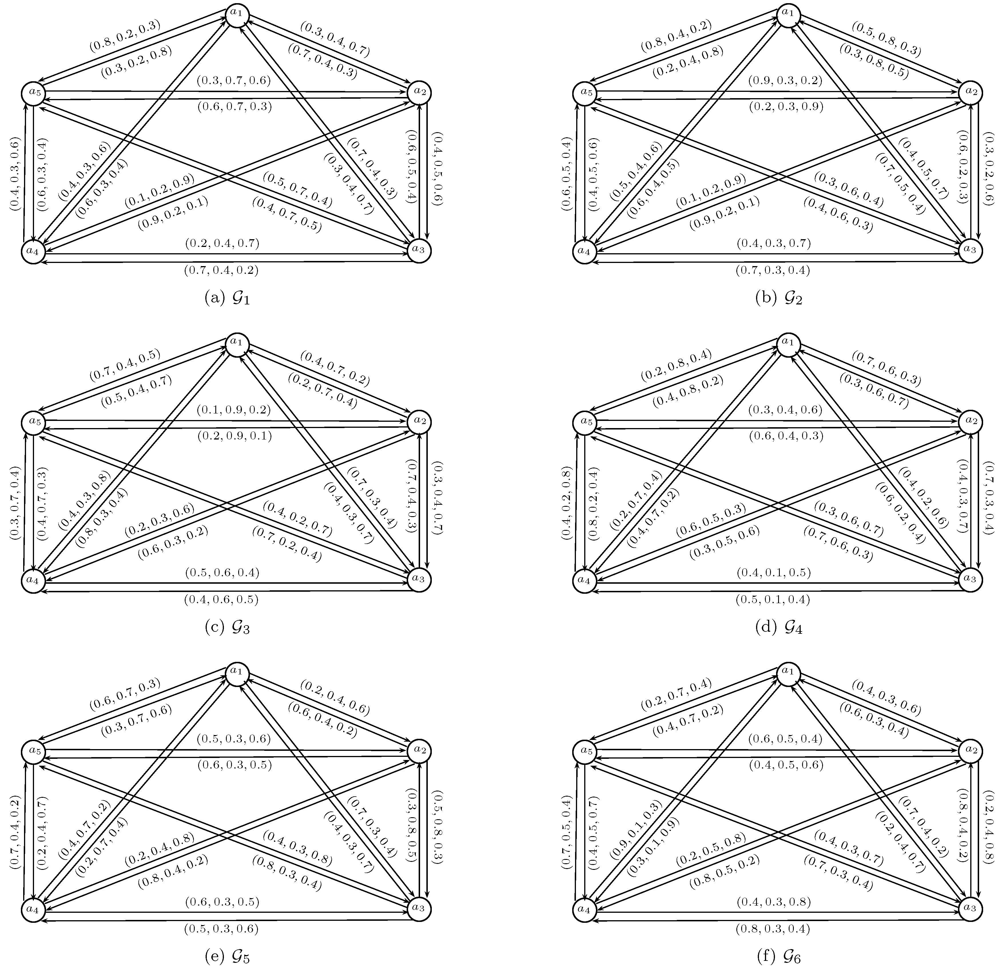
After different meetings, five transnational organizations might want to set up a significant union with (NBP: they are Bank of Maharshtra (BM) $a_1$; Sindh Bank (SB) $a_2$; Dubai Islami Bank (DIB) $a_3$; Islamic Development Bank (IsDB) $a_4$; and the International Exchange Bank (IEB) $a_5$. To choose a suitable critical union accomplice, six experts $e_t(t=1,2,\cdots ,6)$ are welcome to take an interest in a choice examination, who originate from (NBP). In light of their encounters, the experts analyze each pair of choices and give singular decisions utilizing the accompanying SFPRs $R_t={\left(r_{pq}^{\left(t\right)}\right)}_{5\times 5}(t=1,2,\cdots ,6).$ The spherical fuzzy digraphs $G_t$ corresponding to SFPRs $R_t(t=1,2,\cdots ,6)$ given below, are shown in Figure 18.

$$R_1=\left[\begin{array}{ccccc}(0.5,0.5,0.5)& (0.3,0.4,0.7)& (0.7,0.4,0.3)& (0.6,0.3,0.4)& (0.8,0.2,0.3)\\ (0.7,0.4,0.3)& (0.5,0.5,0.5)& (0.4,0.5,0.6)& (0.9,0.2,0.1)& (0.6,0.7,0.3)\\ (0.3,0.4,0.7)& (0.6,0.5,0.4)& (0.5,0.5,0.5)& (0.7,0.4,0.2)& (0.4,0.7,0.5)\\ (0.4,0.3,0.6)& (0.1,0.2,0.9)& (0.2,0.4,0.7)& (0.5,0.5,0.5)& (0.4,0.3,0.6)\\ (0.3,0.2,0.8)& (0.3,0.7,0.6)& (0.5,0.7,0.4)& (0.6,0.3,0.4)& (0.5,0.5,0.5)\end{array}\right],$$

$$R_2=\left[\begin{array}{ccccc}(0.5,0.5,0.5)& (0.5,0.8,0.3)& (0.4,0.5,0.7)& (0.6,0.4,0.5)& (0.8,0.4,0.2)\\ (0.3,0.8,0.5)& (0.5,0.5,0.5)& (0.3,0.2,0.6)& (0.9,0.2,0.1)& (0.2,0.3,0.9)\\ (0.7,0.5,0.4)& (0.6,0.2,0.3)& (0.5,0.5,0.5)& (0.7,0.3,0.4)& (0.4,0.6,0.3)\\ (0.5,0.4,0.6)& (0.1,0.2,0.9)& (0.4,0.3,0.7)& (0.5,0.5,0.5)& (0.6,0.5,0.4)\\ (0.2,0.4,0.8)& (0.9,0.3,0.2)& (0.3,0.6,0.4)& (0.4,0.5,0.6)& (0.5,0.5,0.5)\end{array}\right],$$

$$R_3=\left[\begin{array}{ccccc}(0.5,0.5,0.5)& (0.4,0.7,0.2)& (0.7,0.3,0.4)& (0.8,0.3,0.4)& (0.7,0.4,0.5)\\ (0.2,0.7,0.4)& (0.5,0.5,0.5)& (0.3,0.4,0.7)& (0.6,0.3,0.2)& (0.2,0.9,0.1)\\ (0.4,0.3,0.7)& (0.7,0.4,0.3)& (0.5,0.5,0.5)& (0.4,0.6,0.5)& (0.7,0.2,0.4)\\ (0.4,0.3,0.8)& (0.2,0.3,0.6)& (0.5,0.6,0.4)& (0.5,0.5,0.5)& (0.3,0.7,0.4)\\ (0.5,0.4,0.7)& (0.1,0.9,0.2)& (0.4,0.2,0.7)& (0.4,0.7,0.3)& (0.5,0.5,0.5)\end{array}\right],$$

$$R_4=\left[\begin{array}{ccccc}(0.5,0.5,0.5)& (0.7,0.6,0.3)& (0.4,0.2,0.6)& (0.4,0.7,0.2)& (0.2,0.8,0.4)\\ (0.3,0.6,0.7)& (0.5,0.5,0.5)& (0.7,0.3,0.4)& (0.3,0.5,0.6)& (0.6,0.4,0.3)\\ (0.6,0.2,0.4)& (0.4,0.3,0.7)& (0.5,0.5,0.5)& (0.5,0.1,0.4)& (0.7,0.6,0.3)\\ (0.2,0.7,0.4)& (0.6,0.5,0.3)& (0.4,0.1,0.5)& (0.5,0.5,0.5)& (0.4,0.2,0.8)\\ (0.4,0.8,0.2)& (0.3,0.4,0.6)& (0.3,0.6,0.7)& (0.8,0.2,0.4)& (0.5,0.5,0.5)\end{array}\right],$$

$$R_5=\left[\begin{array}{ccccc}(0.5,0.5,0.5)& (0.2,0.4,0.6)& (0.7,0.3,0.4)& (0.2,0.7,0.4)& (0.6,0.7,0.3)\\ (0.6,0.4,0.2)& (0.5,0.5,0.5)& (0.5,0.8,0.3)& (0.8,0.4,0.2)& (0.6,0.3,0.5)\\ (0.4,0.3,0.7)& (0.3,0.8,0.5)& (0.5,0.5,0.5)& (0.5,0.3,0.6)& (0.8,0.3,0.4)\\ (0.4,0.7,0.2)& (0.2,0.4,0.8)& (0.6,0.3,0.5)& (0.5,0.5,0.5)& (0.7,0.4,0.2)\\ (0.3,0.7,0.6)& (0.5,0.3,0.6)& (0.4,0.3,0.8)& (0.2,0.4,0.7)& (0.5,0.5,0.5)\end{array}\right],$$

$$R_6=\left[\begin{array}{ccccc}(0.5,0.5,0.5)& (0.4,0.3,0.6)& (0.7,0.4,0.2)& (0.3,0.1,0.9)& (0.2,0.7,0.4)\\ (0.6,0.3,0.4)& (0.5,0.5,0.5)& (0.2,0.4,0.8)& (0.8,0.5,0.2)& (0.4,0.5,0.6)\\ (0.2,0.4,0.7)& (0.8,0.4,0.2)& (0.5,0.5,0.5)& (0.8,0.3,0.4)& (0.7,0.3,0.4)\\ (0.9,0.1,0.3)& (0.2,0.5,0.8)& (0.4,0.3,0.8)& (0.5,0.5,0.5)& (0.7,0.5,0.4)\\ (0.4,0.7,0.2)& (0.6,0.5,0.4)& (0.4,0.3,0.7)& (0.4,0.5,0.7)& (0.5,0.5,0.5)\end{array}\right].$$

We use the accumulation operator to combine all the individual SFPRs $R_t={\left(r_{pq}^{\left(t\right)}\right)}_{5\times 5}(t=1,2,3,4,5,6)$ into the collective $R={\left(r_{pq}\right)}_{5\times 5}.$ Here, we use spherical fuzzy weighted averagingSFWA operator [41] to combine the individual SFPR. Thus, we have

$$SFWA(r_{pq}^{\left(1\right)},r_{pq}^{\left(2\right)},\cdots ,r_{pq}^{\left(t\right)})=\left(\sqrt{1-{\left(\prod _{s=1}^t(1-{\left({\alpha }_{pq}^2\right)}^{\left(s\right)})\right)}^{\frac{1}{t}}},{\left(\prod _{s=1}^t\left({\gamma }_{pq}^{\left(s\right)}\right)\right)}^{\frac{1}{t}},{\left(\prod _{s=1}^t({\beta }_{pq}^{\left(s\right)}+{\gamma }_{pq}^{\left(s\right)})\right)}^{\frac{1}{t}}-{\left(\prod _{s=1}^t\left({\gamma }_{pq}^{\left(s\right)}\right)\right)}^{\frac{1}{t}}\right),$$

where

$$\begin{array}{cc}\hfill & \sqrt{1-{\left(\prod _{s=1}^t(1-{\left({\alpha }_{12}^2\right)}^{\left(s\right)})\right)}^{\frac{1}{t}}}\hfill \\ \hfill =& \sqrt{1-{\left((1-{\left(0.3\right)}^2)(1-{\left(0.5\right)}^2)(1-{\left(0.4\right)}^2)(1-{\left(0.7\right)}^2)(1-{\left(0.2\right)}^2)(1-{\left(0.4\right)}^2)\right)}^{\frac{1}{6}}}\hfill \\ \hfill =& \sqrt{1-{\left((1-0.09)(1-0.25)(1-0.16)(1-0.49)(1-0.04)(1-0.16)\right)}^{0.17}}\hfill \\ \hfill =& \sqrt{1-{\left(\left(0.91\right)\left(0.75\right)\left(0.84\right)\left(0.51\right)\left(0.96\right)\left(0.84\right)\right)}^{0.17}}\hfill \\ \hfill =& 0.4667,\hfill \\ \hfill {\left(\prod _{s=1}^t\left({\gamma }_{12}^{\left(s\right)}\right)\right)}^{\frac{1}{t}}& ={(0.4\times 0.8\times 0.7\times 0.6\times 0.4\times 0.3)}^{\frac{1}{6}}\hfill \\ \hfill & ={\left(0.016128\right)}^{0.17}\hfill \\ \hfill & =0.4958,\hfill \\ \hfill {\left(\prod _{s=1}^t({\beta }_{12}^{\left(s\right)}+{\gamma }_{12}^{\left(s\right)})\right)}^{\frac{1}{t}}-{\left(\prod _{s=1}^t\left({\gamma }_{12}^{\left(s\right)}\right)\right)}^{\frac{1}{t}}& ={\left((0.7+0.4)(0.3+0.8)(0.2+0.7)(0.3+0.6)(0.6+0.4)(0.6+0.3)\right)}^{\frac{1}{6}}-0.4958\hfill \\ \hfill & ={\left(\left(1.1\right)\left(1.1\right)\left(0.9\right)\left(0.9\right)\left(1.0\right)\left(0.9\right)\right)}^{0.17}-0.4958\hfill \\ \hfill & =0.9789-0.4958\hfill \\ \hfill & =0.4831.\hfill \end{array}$$

We find the collective SFPR:

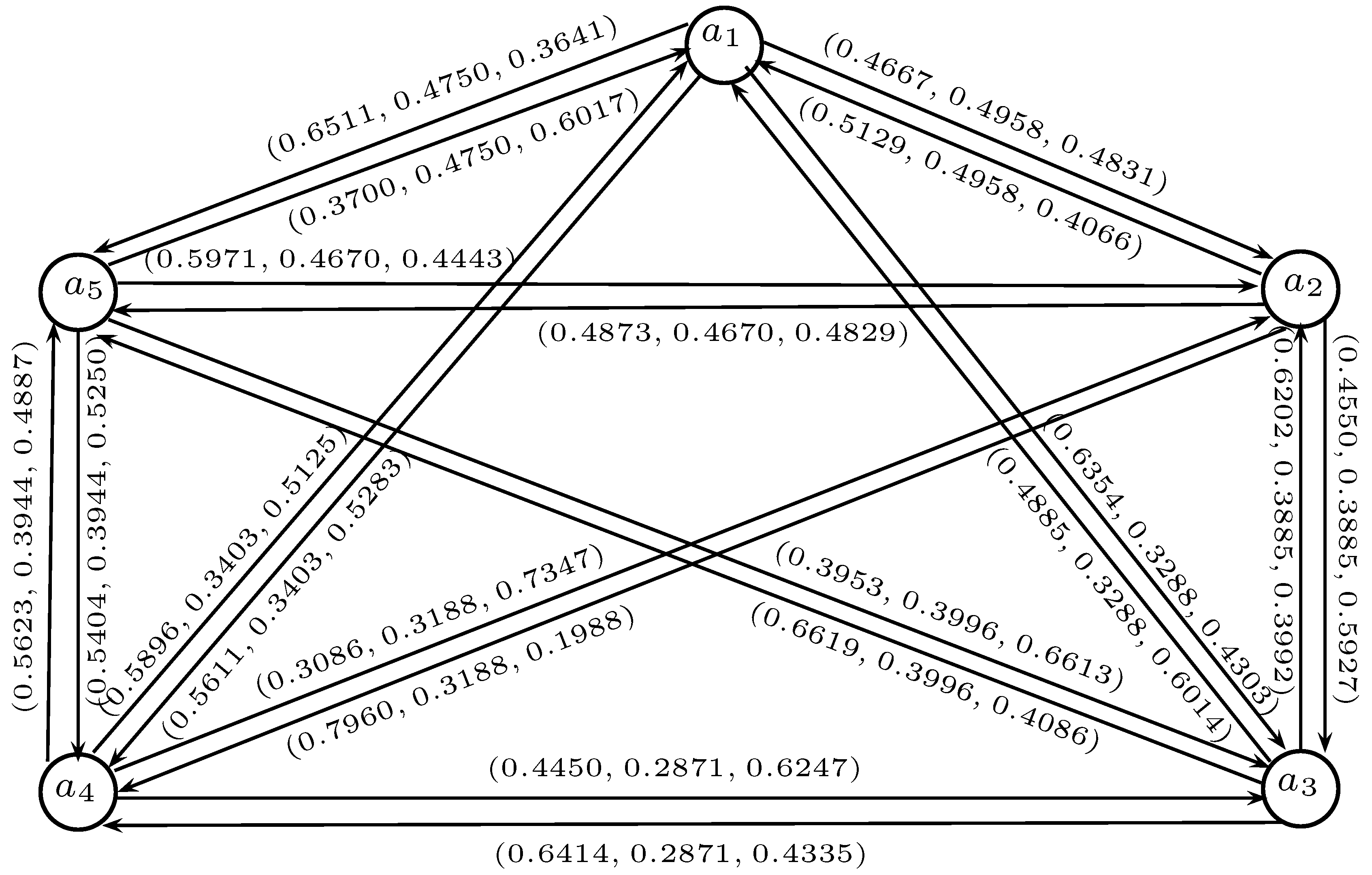
$$R=\left[\begin{array}{ccccc}(0.5000,0.5000,0.5000)& (0.4667,0.4958,0.4831)& (0.6354,0.3288,0.4303)& (0.5611,0.3403,0.5283)& (0.6511,0.4750,0.3641)\\ (0.5129,0.4958,0.4066)& (0.5000,0.5000,0.5000)& (0.4550,0.3885,0.5927)& (0.7960,0.3188,0.1988)& (0.4873,0.4670,0.4829)\\ (0.4885,0.3288,0.6014)& (0.6202,0.3885,0.3992)& (0.5000,0.5000,0.5000)& (0.6414,0.2871,0.4335)& (0.6619,0.3996,0.4086)\\ (0.5896,0.3403,0.5125)& (0.3086,0.3188,0.7347)& (0.4450,0.2871,0.6247)& (0.5000,0.5000,0.5000)& (0.5623,0.3944,0.4887)\\ (0.3700,0.4750,0.6017)& (0.5971,0.4670,0.4443)& (0.3953,0.3996,0.6613)& (0.5404,0.3944,0.5250)& (0.5000,0.5000,0.5000)\end{array}\right].$$

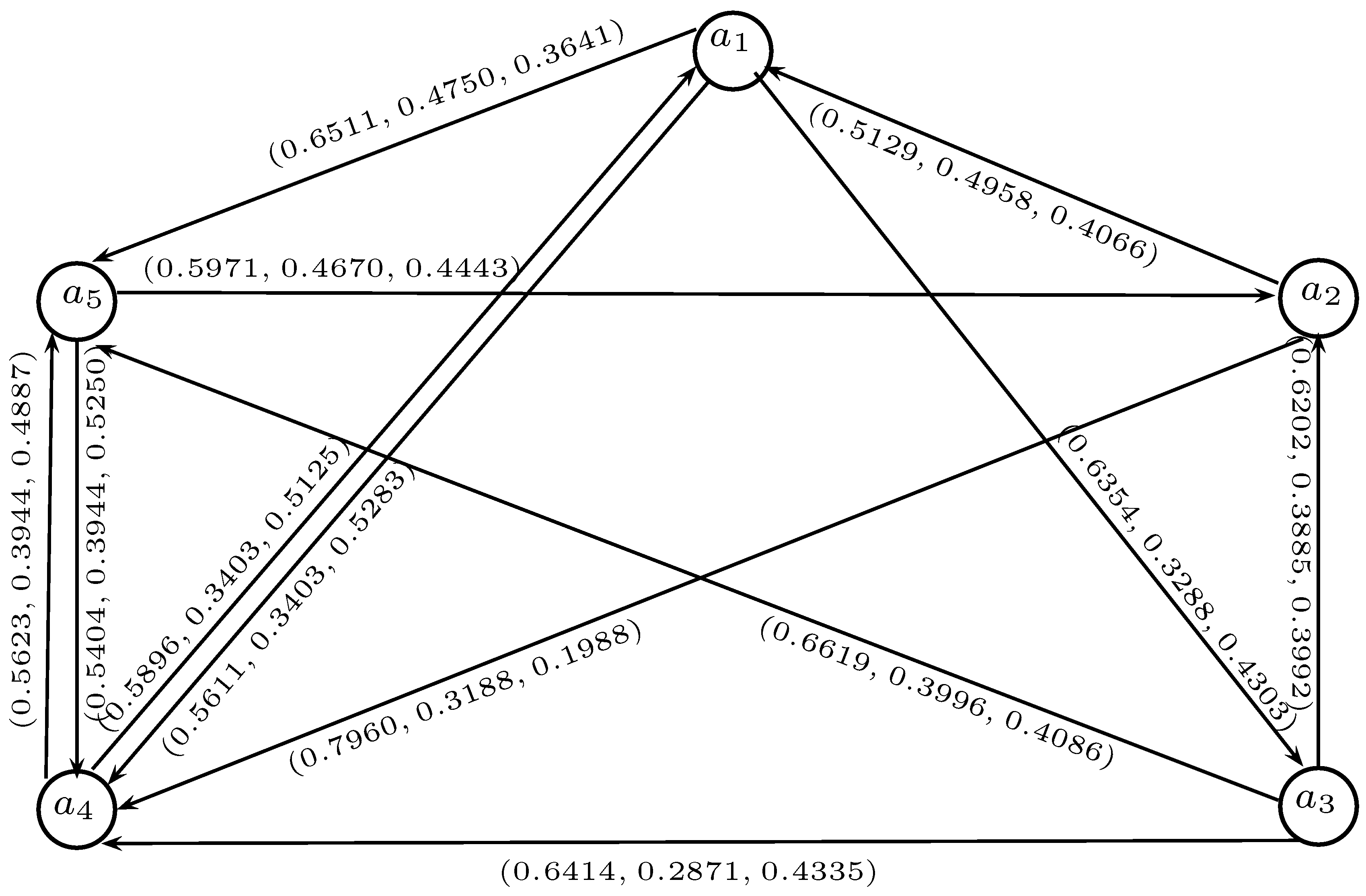
In the directed model relating to a collective SFPR above, as shown in Figure 19, we select those spherical fuzzy numbers whose truthness degrees ${\alpha }_{pq}\ge 0.5(p,q=1,2,3,4,5),$ and resulting partial model is shown in Figure 20.

We compute the out-degrees out-$d\left(a_p\right)(p=1,2,3,4,5)$ in a partial directed model as follows:

$$\begin{array}{cc}\hfill \mathrm{out}-d\left(a_1\right)& =(1.8476,1.1441,1.3227),\mathrm{out}-d\left(a_2\right)=(1.3089,0.8146,0.6054),\mathrm{out}-d\left(a_3\right)=(1.9235,1.0752,1.2413),\hfill \\ \hfill \mathrm{out}-d\left(a_4\right)& =(1.1519,0.7347,1.0012),\mathrm{out}-d\left(a_5\right)=(1.1375,0.8594,0.9693).\hfill \end{array}$$

As indicated by the truthness degrees of out-$d\left(a_p\right)(p=1,2,3,4,5),$ we have the positioning of the variables $a_p(p=1,2,3,4,5)$ as:

$$a_3\succ a_1\succ a_2\succ a_4\succ a_5.$$

Thus, the best choice is $a_3.$

Now, using a spherical fuzzy weighted geometric (SFWG) operator [41],

$$SFWG(r_{pq}^{\left(1\right)},r_{pq}^{\left(2\right)},\cdots ,r_{pq}^{\left(t\right)})=\left({\left(\prod _{s=1}^t({\alpha }_{pq}^{\left(s\right)}+{\gamma }_{pq}^{\left(s\right)})\right)}^{\frac{1}{t}}-{\left(\prod _{s=1}^t\left({\gamma }_{pq}^{\left(s\right)}\right)\right)}^{\frac{1}{t}},{\left(\prod _{s=1}^t\left({\gamma }_{pq}^{\left(s\right)}\right)\right)}^{\frac{1}{t}},\sqrt{1-{\left(\prod _{s=1}^t(1-{\left({\beta }_{pq}^2\right)}^{\left(s\right)})\right)}^{\frac{1}{t}}}\right),$$

we find the collective SFPR:

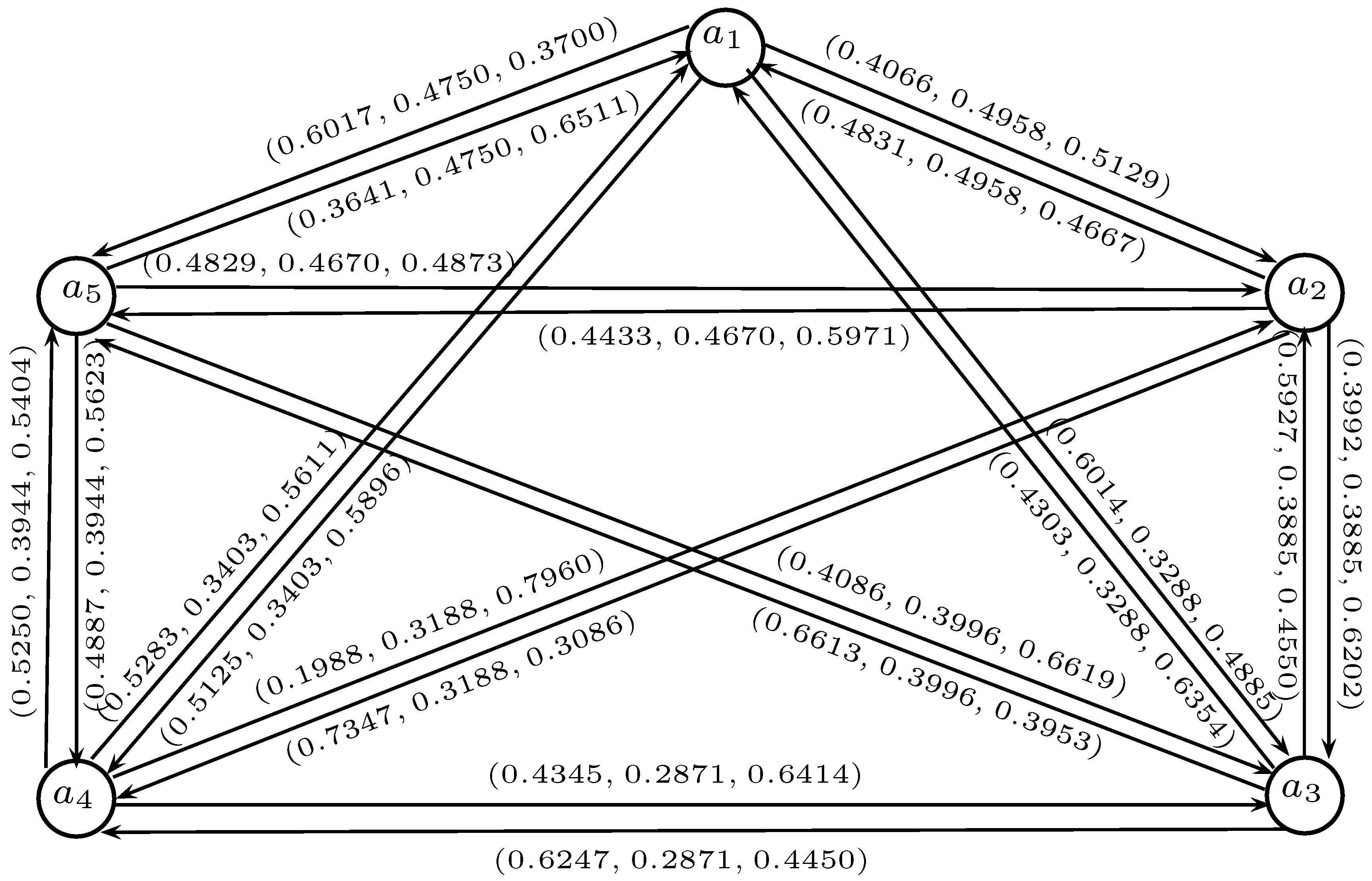
$$R=\left[\begin{array}{ccccc}(0.5000,0.5000,0.5000)& (0.4066,0.4958,0.5129)& (0.6014,0.3288,0.4885)& (0.5125,0.3403,0.5896)& (0.6017,0.4750,0.3700)\\ (0.4831,0.4958,0.4667)& (0.5000,0.5000,0.5000)& (0.3992,0.3885,0.6202)& (0.7347,0.3188,0.3086)& (0.4433,0.4670,0.5971)\\ (0.4303,0.3288,0.6354)& (0.5927,0.3885,0.4550)& (0.5000,0.5000,0.5000)& (0.6247,0.2871,0.4450)& (0.6613,0.3996,0.3953)\\ (0.5283,0.3403,0.5611)& (0.1988,0.3188,0.7960)& (0.4345,0.2871,0.6414)& (0.5000,0.5000,0.5000)& (0.5250,0.3944,0.5404)\\ (0.3641,0.4750,0.6511)& (0.4829,0.4670,0.4873)& (0.4086,0.3996,0.6619)& (0.4887,0.3944,0.5623)& (0.5000,0.5000,0.5000)\end{array}\right].$$

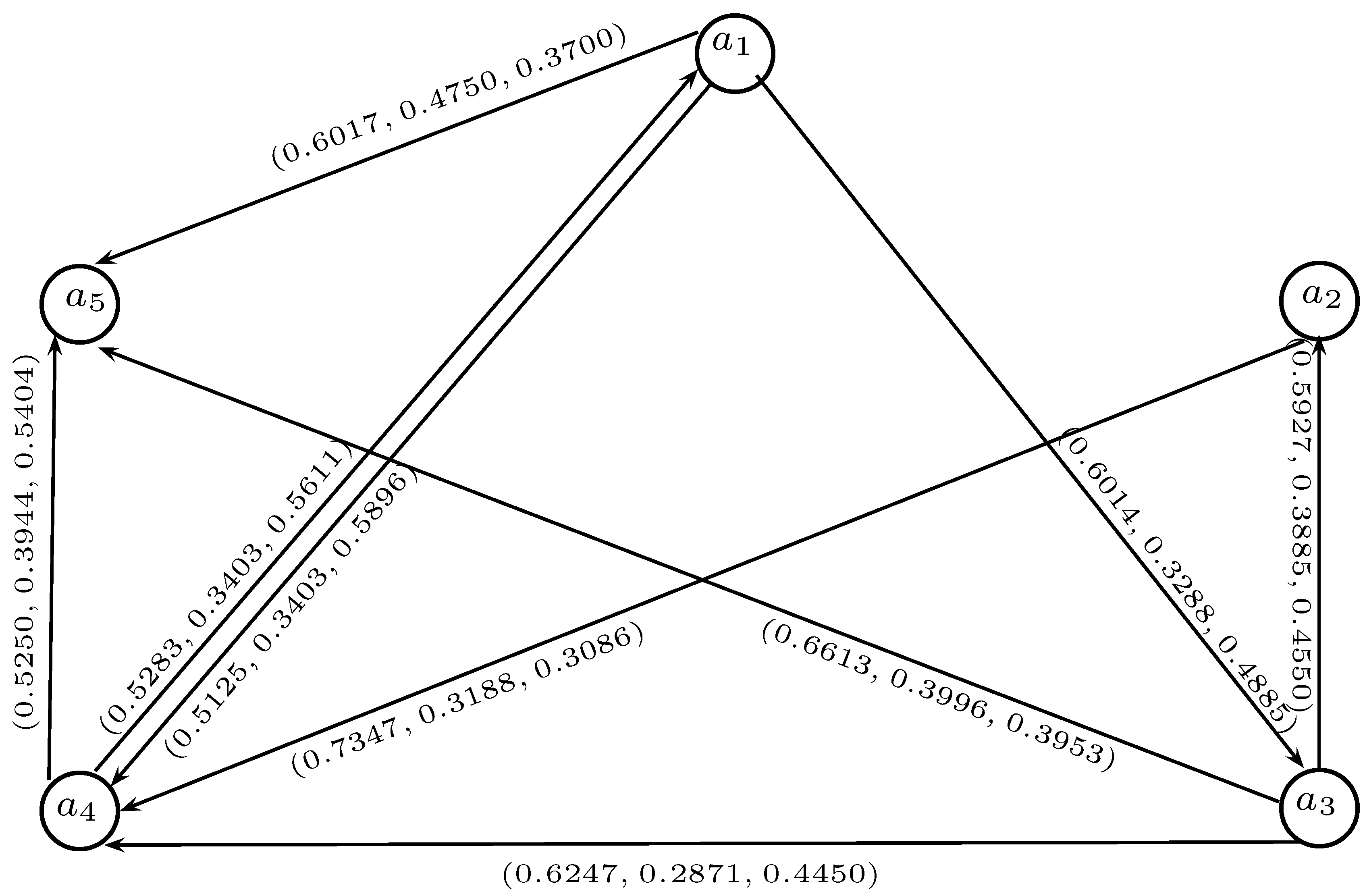
In the directed model relating to a collective SFPR above, as shown in Figure 21, we select those spherical fuzzy numbers whose truthness degrees ${\alpha }_{pq}\ge 0.5(p,q=1,2,3,4,5),$ and resulting partial model is shown in Figure 22.

We compute the out-degrees out-$d\left(a_p\right)(q=1,2,3,4,5)$ in a partial directed model as follows:

$$\begin{array}{cc}\hfill \mathrm{out}-d\left(a_1\right)& =(1.7156,1.1440,1.4481),\hfill \\ \hfill \mathrm{out}-d\left(a_2\right)& =(0.7347,0.3188,0.3086),\hfill \\ \hfill \mathrm{out}-d\left(a_3\right)& =(1.8787,1.0752,1.2953),\hfill \\ \hfill \mathrm{out}-d\left(a_4\right)& =(1.0533,0.7347,1.1015),\hfill \\ \hfill \mathrm{out}-d\left(a_5\right)& =(0.0000,0.0000,0.0000).\hfill \end{array}$$

As indicated by the truthness degrees of out-$d\left(a_p\right)(p=1,2,3,4,5),$ we have the positioning of the variables $a_p(p=1,2,3,4,5)$ as:

$$a_3\succ a_1\succ a_4\succ a_2\succ a_5.$$

Thus, the best choice is Dubai Islami Bank (DIB) $a_3.$

5. Comparative Analysis

Spherical fuzzy sets are an extension of PFS, as they provides enlargement of the space of degrees of truthness $\left(\alpha \right),$ abstinence $\left(\gamma \right)$, and falseness $\left(\beta \right)$ in the interval $[0,1]$, with the condition $0\le {\alpha }^2+{\gamma }^2+{\beta }^2\le 1.$ Picture fuzzy sets which were proposed by Cuong [4,5] have been studied widely by various researchers, but the range of applicability of PFS is limited due to its constraint $0\le \alpha +\gamma +\beta \le 1.$ Under this condition, PFSs cannot express some decision evaluation information effectively; as a decision-maker may provide information for a particular attribute, such that the sum of the degrees of truthness, abstinence, and falseness become greater than one.

In order to solve such types of problems, SFSs were defined by Gündogdu and Kahraman [16] in 2018, whose prominent characteristic is that the square sum of the truthness, abstinence, and falseness degrees is less than or equal to one. Thus, an SFS can solve a number of practical problems that cannot be handled using a PFS. The flexibility and the effectiveness of an SF model can be proved by the following example: If a decision maker provides the degrees of truthness, abstinence, and falseness as $0.4,0.6$, and $0.5,$ respectively. It is readily seen that $0.4+0.6+0.5>1,$ while ${0.4}^2+{0.6}^2+{0.5}^2\le 1.$ Thus this situation cannot be illustrated by PFS. However, it is appropriate to apply SFS. Thus, the SFS model is considerably more close to human thinking than those of prior concepts. The literature shows that another extension is suggested by Li et al. [18] in 2018, known as q-rung picture fuzzy set (q-RPFS). This proposed concept further relaxes the constraints of picture and spherical fuzzy sets with $0\le {\alpha }^q+{\gamma }^q+{\beta }^q\le 1,q\ge 1.$

It is noteworthy that the class of q-RPFSs extends the classes of PFSs and SFSs. Thus, it can express vague information more flexibly and accurately with increasing q rungs. When $q=1,$ this model reduces to the PF model, and when $q=2,$ it becomes the SF model. Thus, a wider range of uncertain information can be expressed using the methods proposed in this paper, which are closer to real decision-making. This helps us to deal with MCDM problems and to sketch real scenarios more accurately. Hence our approach towards MCDM is more flexible and generalized, which provides a vast space of acceptable triplets given by decision-makers, according to the different attitudes, as compared to the PF model.

6. Conclusions

Spherical fuzzy models deal with uncertainty problems more efficiently, with the constraint $0\le {\alpha }^2+{\gamma }^2+{\beta }^2\le 1$, providing a vast space to appoint degrees of one’s own choice as compared to the picture fuzzy model. As fuzzy graph theory can deal with ambiguous and vague notions in a natural way, and thus has a large number of applications in modeling such real-life systems where the levels of information inherent in the system varies with different levels of precision. In graph-theoretical concepts, to tackle the situations when human opinions are of types: yes, abstain, no, and refusal, the proposed model can well express evaluation information in a broad manner.

In this research article, we have discussed some operations on SFGs and developed several results related to their degrees and total degrees. Further, we have described certain novel concepts of SFGs, such as irregularity and edge irregularity with illustrative examples. For the validity of these properties, some necessary and sufficient conditions are proposed. These properties allow one to deal with the many challenges associated with the analysis of graphs. As the DM problems in fuzzy models present themselves to the various organs of the state, we have developed an MCGDM problem regarding the selection of the best critical union accomplice in the NBP using SFGs. The applications of SFGs serve us with innovative and optimal results that seem to be highly significant as they give directions to MCDM. In the future, we plan to extend this study to (i) spherical fuzzy hypergraphs; (ii) hesitant spherical fuzzy graphs; (iii) single-valued neurotrophic spherical graphs; and (iv) complex spherical fuzzy Hamacher aggregation operators.

References

1. Zadeh, L.A. Fuzzy sets. Inf. Control 1965, 8, 338–353. [Google Scholar] [CrossRef] [Green Version]
2. Atanassov, K.T. Intuitionistic fuzzy sets. Fuzzy Sets Syst. 1986, 20, 87–96. [Google Scholar] [CrossRef]
3. Yager, R.R. Pythagorean membership grades in multi-criteria decision making. IEEE Trans. Fuzzy Syst. 2014, 22, 958–965. [Google Scholar] [CrossRef]
4. Cuong, B.C. Picture fuzzy sets—First results, Part 1. In Seminar Neuro-Fuzzy Systems with Applications; Institute of Mathematics, Vietnam Academy of Science and Technology: Hanoi, Vietnam, 2013. [Google Scholar]
5. Cuong, B.C. Picture fuzzy sets—First results, Part 2. In Seminar Neuro-Fuzzy Systems with Applications; Institute of Mathematics, Vietnam Academy of Science and Technology: Hanoi, Vietnam, 2013. [Google Scholar]
6. Zeng, S.; Asharf, S.; Arif, M.; Abdullah, S. Application of exponential Jensen picture fuzzy divergence measure in multi-criteria group decision making. Mathematics 2019, 7, 191. [Google Scholar] [CrossRef] [Green Version]
7. Garg, H. Some picture fuzzy aggregation operators and their applications to multicriteria decision-making. Arab. J. Sci. Eng. 2017, 42, 5275–5290. [Google Scholar] [CrossRef]
8. Liu, M.; Zeng, S.; Baležentis, T.; Streimikiene, D. Picture Fuzzy Weighted Distance Measures and Their Application to Investment Selection. Amfiteatru Econ. 2019, 21, 682. [Google Scholar] [CrossRef]
9. Zhang, H.; Zhang, R.; Huang, H.; Wang, J. Some picture fuzzy Dombi Heronian mean operators with their application to multi-attribute decision-making. Symmetry 2018, 10, 593. [Google Scholar] [CrossRef] [Green Version]
10. Cuong, B.C. Picture fuzzy sets. J. Comput. Sci. Cybern. 2014, 30, 409–420. [Google Scholar]
11. Cuong, B.C.; Kreinovich, V. Picture fuzzy sets: A new concept for computational intelligence problems. In Proceedings of the Third World Congress on Information and Communication Technologies, Hanoi, Vietnam, 15–18 December 2013. [Google Scholar]
12. Cuong, B.C.; Hai, P.V. Some fuzzy logic operators for picture fuzzy sets. In Proceedings of the Seventh International Conference on Knowledge and Systems Engineering, HoChiMinh City, Vietnam, 8–10 October 2015. [Google Scholar]
13. Cuong, B.C.; Kreinovich, V.; Ngan, R.T. A classification of representable t-norm operators for picture fuzzy sets. In Proceedings of the Eighth International Conference on Knowledge and Systems Engineering, Hanoi, Vietnam, 6–8 October 2016. [Google Scholar]
14. Singh, P. Correlation coefficients for picture fuzzy sets. J. Intell. Fuzzy Syst. 2015, 28, 591–604. [Google Scholar] [CrossRef]
15. Wei, G. Some similarity measures for picture fuzzy sets and their applications. Iran. J. Fuzzy Syst. 2018, 15, 77–89. [Google Scholar]
16. Gündogdu, F.K.; Kahraman, C. Spherical fuzzy sets and spherical fuzzy TOPSIS method. J. Intell. Fuzzy Syst. 2018, 36, 1–16. [Google Scholar]
17. Ashraf, S.; Abdulla, S.; Mahmood, T.; Ghani, F.; Mahmood, T. Spherical fuzzy sets and their applications in multi-attribute decision making problems. J. Intell. Fuzzy Syst. 2018. [Google Scholar] [CrossRef]
18. Li, L.; Zhang, R.; Wang, J.; Shang, X.; Bai, K. A novel approach to multi-attribute group decision-making with q-rung picture linguistic information. Symmetry 2018, 10, 172. [Google Scholar] [CrossRef] [Green Version]
19. Kaufmann, A. Introduction a la Theorie des Sour-ensembles Flous; Masson et Cie: Paris, France, 1973. [Google Scholar]
20. Zadeh, L.A. Similarity relations and fuzzy orderings. Inf. Sci. 1971, 3, 177–200. [Google Scholar] [CrossRef]
21. Rosenfeld, A. Fuzzy graphs. In Fuzzy Sets and Their Applications to Cognitive and Decision Processes; Academic Press: New York, NY, USA, 1975; pp. 77–95. [Google Scholar]
22. Bhattacharya, P. Some remarks on fuzzy graphs. Pattern Recognit. Lett. 1987, 6, 297–302. [Google Scholar] [CrossRef]
23. Santhimaheswari, N.R.; Sekar, C. On strongly edge irregular fuzzy graphs. Kragujev. J. Math. 2016, 40, 125–135. [Google Scholar] [CrossRef]
24. Al-Hawary, T. Certain classes of fuzzy graphs. Eur. J. Pure Appl. Math. 2017, 10, 552–560. [Google Scholar]
25. Al-Hawary, T. Complete fuzzy graphs. Int. J. Math. Combin. 2011, 4, 26–34. [Google Scholar]
26. Al-Hawary, T. On balanced graphs and balanced matroids. Math. Sci. Res. Hot-Line 2000, 4, 35–45. [Google Scholar]
27. Al-Hawary, T.; Mahmood, T.; Jan, N.; Ullah, K.; Hussain, A. On intuitionistic fuzzy graphs and some operations on picture fuzzy graphs. Ital. J. Pure Appl. Math. To appear.
28. Karunambigai, M.G.; Parvathi, R. Intuitionistic fuzzy graphs. In Proceedings of the International Conference 9th Fuzzy Days, Dortmund, Germany, 18–20 September 2006; pp. 139–150. [Google Scholar]
29. Akram, M.; Davvaz, B. Strong intuitionistic fuzzy graphs. Filomat 2012, 26, 177–196. [Google Scholar] [CrossRef] [Green Version]
30. Naz, S.; Ashraf, S.; Akram, M. A novel approach to decision-making with Pythagorean fuzzy information. Mathematics 2018, 6, 95. [Google Scholar] [CrossRef] [Green Version]
31. Akram, M.; Habib, A.; Ilyas, F.; Dar, J.M. Specific types of Pythagorean fyzzy graphs and application to decision-making. Math. Comput. Appl. 2018, 23, 42. [Google Scholar]
32. Akram, M. Decision Making Method Based on Spherical Fuzzy Graphs. In Studies in Fuzziness and Soft Computing; Kahraman, C., Otay, I., Eds.; Springer: Berlin, Germany, 2020. [Google Scholar]
33. Akram, M.; Habib, A. q-Rung picture fuzzy graphs: A creative view on regularity with applications. J. Appl. Math. Comput. 2019, 61, 235–280. [Google Scholar] [CrossRef]
34. Akram, M.; Habib, A.; Koam, A.N.A. A Novel Description on Edge-Regular q-Rung Picture Fuzzy Graphs with Application. Symmetry 2019, 11, 489. [Google Scholar] [CrossRef] [Green Version]
35. Zeng, S.; Chen, S.M.; Kuo, L.W. Multiattribute decision making based on novel score function of intuitionistic fuzzy values and modified VIKOR method. Inf. Sci. 2019, 488, 76–92. [Google Scholar] [CrossRef]
36. Zeng, S.; Chen, S.M.; Fan, K.Y. Interval-valued intuitionistic fuzzy multiple attribute decision making based on nonlinear programming methodology and TOPSIS method. Inf. Sci. 2020, 506, 424–442. [Google Scholar] [CrossRef]
37. Akram, M.; Habib, A.; Davvaz, B. Direct sum of n Pythagorean fuzzy graphs with application to group decision-making. J. Mult. Valued Log. Soft Comput. 2019, 33, 75–115. [Google Scholar]
38. Akram, M.; Dar, J.M.; Farooq, A. Planar graphs under Pythagorean fuzzy environment. Mathematics 2018, 6, 278. [Google Scholar] [CrossRef] [Green Version]
39. Akram, M.; Naz, S. Energy of Pythagorean fuzzy graphs with applications. Mathematics 2018, 6, 136. [Google Scholar] [CrossRef] [Green Version]
40. Habib, A.; Akram, M.; Farooq, A. q-Rung orthopair fuzzy competition graphs with application in the soil ecosystem. Mathematics 2019, 7, 91. [Google Scholar] [CrossRef] [Green Version]
41. Ashraf, S.; Abdullah, S.; Mahmood, T. Spherical fuzzy Dombi aggregation operators and their application in group decision making problems. J. Ambient Intell. Humaniz. Comput. 2019. [Google Scholar] [CrossRef]
Figure 1. Comparison of the spaces of picture fuzzy sets (PFSs) and spherical fuzzy sets (SFSs).
Mca 25 00008 g001
Figure 2. Spherical fuzzy graphs (SFGs).
Mca 25 00008 g002
Figure 3. G 1 G 2 .
Mca 25 00008 g003
Figure 4. SFGs.
Mca 25 00008 g004
Figure 5. G 1 | G 2 .
Mca 25 00008 g005
Figure 6. I-SFG G .
Mca 25 00008 g006
Figure 7. TI-SFG G .
Mca 25 00008 g007
Figure 8. Strongly I-SFG G .
Mca 25 00008 g008
Figure 9. Highly TI-SFG G .
Mca 25 00008 g009
Figure 10. SFG G .
Mca 25 00008 g010
Figure 11. SFG G .
Mca 25 00008 g011
Figure 12. SFG G .
Mca 25 00008 g012
Figure 13. Strongly EI-SFG G .
Mca 25 00008 g013
Figure 14. Strongly edge TI-SFG G .
Mca 25 00008 g014
Figure 15. SFG G .
Mca 25 00008 g015
Figure 16. SFG G .
Mca 25 00008 g016
Figure 17. I-SFG G .
Mca 25 00008 g017
Figure 18. Spherical fuzzy digraphs.
Mca 25 00008 g018
Figure 19. Directed model of the combined SFPR.
Mca 25 00008 g019
Figure 20. Partial directed model of the combined SFPR.
Mca 25 00008 g020
Figure 21. Directed model of the combined SFPR.
Mca 25 00008 g021
Figure 22. Partial directed model of the combined SFPR.
Mca 25 00008 g022