1. Introduction
The problem of a one-point particle, or an ensemble of non-interacting point particles, moving with constant velocity inside a bounded region, subject to elastic collisions with the boundaries, is generically known as a billiard. Such dynamical systems are described by nonlinear mappings and have great interest in several branches of physics [
1,
2,
3,
4,
5,
6]. Even billiards with simple geometry exhibit rich dynamical behaviors, typical of Hamiltonian systems, and depending on the geometry of the boundaries and the control parameters, the associated phase space can be: I—regular, consisting of quasi-periodic or periodic orbits lying on Kolmogorov–Arnold–Moser (KAM) tori; II—chaotic, with orbits that densely fill the whole phase space; or III—mixed, in which regular motion coexists with chaotic motion. This is the case with most non-integrable Hamiltonian systems, wherein the characterization of orbits as regular or chaotic is of great interest [
7].
As a consequence of mixed phase space, some chaotic orbits that come sufficiently close to a KAM island tend to spend a long time around that region, almost behaving as regular orbits. Following this transient time, these orbits return to the chaotic sea. This phenomenon is known as stickiness and it influences the transport properties of the system [
6,
8,
9,
10].
To distinguish chaotic orbits from regular ones, a standard approach that has been frequently employed is the estimation of Lyapunov exponents [
6,
11]. For conservative systems, regular orbits have null Lyapunov exponents, while chaotic orbits have at least one positive Lyapunov exponent. For Hamiltonian systems, the sum of the exponents must be zero in order to satisfy Liouville’s theorem. In numerical applications, finite-time Lyapunov exponents (FTLEs) [
6,
11,
12,
13] can be calculated, and although they are suitable to investigate systems with a mixed phase space, the existence of stable islands delays the convergence of chaotic orbits, wherein simulations of high computational effort are required to calculate the exponents. The distribution of the FTLEs over initial conditions carries information about the system dynamics. For completely chaotic systems, a Gaussian distribution is expected. If a small amount of regular structures are present in the phase space, the orbits affected by stickiness will have smaller FTLE values, which induces a tail in the distribution, making it asymmetric. If a large amount of regular structures are present, the system has strong sticky motion and the distribution of the FTLEs is multimodal [
14,
15].
In the late 1960s, an interesting and not well-known theorem was proposed by Slater [
16], whose nonlinear version was well adapted in [
6,
17]. It states that it is possible to distinguish quasi-periodic dynamics from chaotic dynamics by analyzing the Poincaré return times, also called recurrence times, and that for any connected interval of size
, there are no more than three different return times, the largest of them being the sum of the other two.
The technique of recurrence plots (RPs) [
18,
19] has been applied for the visualization and analysis of nonlinear experimental data in many different fields, from biological sciences [
20,
21,
22] to complex systems [
23,
24,
25]. This tool was first introduced in the context of dynamical systems to visualize the recurrence of trajectories in the phase space [
19]. As chaotic and quasi-periodic orbits have different recurrence properties, RPs allow us to distinguish the behavior of these orbits, identify the interval of time that a chaotic orbit has been trapped by stickiness, and even quantify stickiness by using recurrence quantification analysis [
26].
Quantum mechanical versions of billiards provide useful models to investigate the quantum properties of certain systems, as it is possible to identify signatures of the structures present in the phase space of their classical analogue in the quantum wave functions [
27,
28,
29]. The distribution of spacings between the neighbor energy levels of a quantum billiard obeys a Poisson distribution for classically integrable systems and a Wigner distribution (or GOE distribution) for classically chaotic systems. In the early 1990s, a billiard with a point-like scatterer was first proposed to investigate the quantum aspects of systems whose corresponding classical limit was between integrable and chaotic. This class of systems is known as singular (or Šeba) billiards [
27] and the distance between its neighbor energy levels obeys a Poisson distribution.
A zero-size scatterer is an idealized limit of a small obstacle [
29]. In this work, we investigate the classical dynamics of a billiard with a very small scatterer through its recurrence properties and estimations of the largest Lyapunov exponent (LLE). The chosen model is the annular billiard, which has been the subject of many analytical and numerical studies [
28,
30,
31,
32,
33,
34,
35]. It consists of a particle confined in the region between two circumscribed circumferences of radii
and
, with
. When the circumferences are concentric, the energy and angular momentum are both conserved and therefore the system is integrable, since the plane billiard has two degrees of freedom. If the circumferences are eccentric, the angular momentum is altered with the collisions with the inner circle and chaotic behavior may be observed. The limit of the very small scatterer is obtained by choosing
and we have called this limit to be a near-singular billiard.
It has been postulated in [
36] that it is not possible to remove the chaotic behavior of chaotic nonlinear systems by reducing the magnitude of the nonlinear part. The author has arrived at this conclusion by examining a few cases of chaotic systems, described by one-dimensional mappings, when the nonlinear part is reduced. This work also aims to verify the validity of this proposition for our model, which is described by a two-dimensional nonlinear mapping.
2. Materials and Methods
In this section we will discuss the annular billiard model, the numerical method applied to estimate the largest Lyapunov exponent and the technique of RPs.
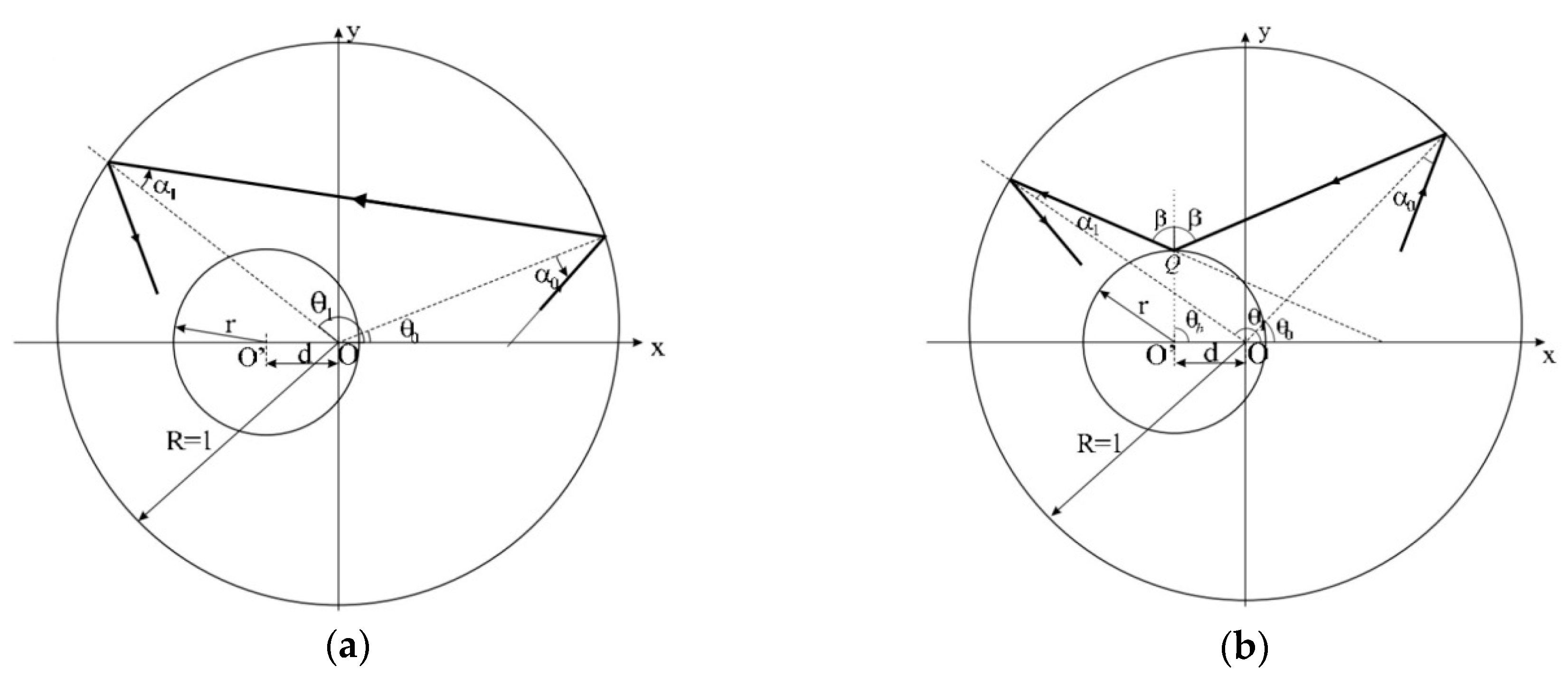
The system of interest consists of a classical particle confined in the annular region limited by two circumscribed circumferences. The geometry may be concentric or eccentric. The radius of the outer circle is defined as
, the radius of the inner circle (the scatterer) as
, and the eccentricity as
. See
Figure 1 for an example of the annular billiard geometry.
On the billiard, a particle moves freely in a straight line with constant velocity until it elastically collides with a boundary. Succeeding a collision, the particle´s trajectory is specularly reflected, i.e., the angle of reflection is equal to the angle of incidence. From
Figure 1, we can see that the position at a collision with the outer boundary is determined by the angle of incidence
and the arc-angle
, for
and
. The map that describes the dynamics projects the coordinates
of a collision with the outer boundary in the coordinates
of the next collision.
There are two kinds of motion which are distinguished by the tangency condition, which reads as follows:
If the combination of
does not satisfy Condition (1), the dynamics is described by the map
and therefore the movement is of type A.
Type A: Between two successive collisions with the outer boundary, the particle does not collide with the scatterer, and so the map
reads as follows:
On the other hand, if Condition (1) is satisfied, the dynamics is described by the map
and therefore the movement is of type B.
Type B: Between two successive collisions with the external circle, the particle collides with the internal circle, and the dynamics is given by
where
The mapping equations have been obtained via geometrical considerations and a more detailed discussion can be found in [
28].
The trajectories that will never cross the caustic (an auxiliary circle centered at the origin, with a radius of ) or never hit the scatterer are the so-called whispering gallery orbits (WGO). In order to keep the phase space area filled by the WGO constant, when varying the eccentricity, the radius of the caustic in the simulations was fixed as . The canonically conjugate pair of variables used to determine the Poincaré section were , with , and , with , collected at every collision with the outer boundary. It is worth emphasizing that is the angular momentum of the particle with respect to the origin of the outer boundary at the moment of collision.
The conditions to generate periodic orbits in the concentric annular billiard are well-known. For trajectories that do not hit the scatterer, the dynamical behavior is the same as in the circular billiard, and the initial condition
generates a periodic orbit if
where
is the period of the orbit and
is the number of turns made by the particle around the billiard. Due to the billiard’s symmetry, any value of
generates an orbit with the same period.
For trajectories that hit the inner boundary, the periodic orbit condition is
The Lyapunov exponents quantify the average expansion or contraction of a small volume of initial conditions. Given a dynamical system represented by the orbit
, with
being the number of the iteration, in a phase space of arbitrary dimension, the stability of the orbit may be verified through the evolution of a satellite orbit named
. Initially, both orbits are separated by an infinitesimal distance
, with
, where the zero index indicates the initial iteration. For chaotic orbits, this distance grows exponentially with time, according to
where
is the exponential expansion rate. This allows us to define the Lyapunov exponent as
This equation estimates the average exponential separation rate between the original orbit and its satellite one. If
is greater than zero, the orbit is chaotic. Otherwise, it is periodic or quasi-periodic.
The numerical procedure to estimate the largest Lyapunov exponent in the annular billiard with the FTLE method can be described as follows: First, we truncate the time evolution at a finite, but long, time. Then, given an initial orbit
and a satellite orbit
, initially separated by the distance
, set as
, we evolve both orbits according to the mapping dynamics. After a defined rescaling time
, we measure the distance between them as
where
and
. The distance between orbits
is used to rescale the satellite orbit in the same direction of the original orbit and then the procedure is restarted with
The FTLE is computed considering
’s successive
time intervals, until the predetermined finite time is reached, with the expression
We will now discuss in a general way the technique of RPs. Once again, given the orbit
, with
being the number of the iteration, we can compute the recurrence matrix,
where
is a predefined threshold,
is the Heaviside function, and
is a norm defining the distance between two points, such that
if
and
if
.
is a binary square matrix, with elements of ‘zeros’ and ‘ones’, and its graphical representation is called a ‘recurrence plot’. The value ‘one’ is encoded by a black point, i.e., the distance between the respective phase space points is smaller than
, which means that at the
i-th iteration the orbit returned to the region of the phase space where it was at the
j-th iteration, after
iterations. The value of ‘zero’ is encoded by a white point, i.e., the distance between the phase space points at the
j-th and
i-th iteration is larger than
, and therefore the orbit had not yet returned to the previously visited reference region of the phase space. A white vertical line between two points provides the recurrence time or Poincaré return time (i.e., the time that takes for the orbit to return to a previous state).
To illustrate the procedure, let us discuss the computation of the first column of the matrix , i.e., consider , so that the returns to the neighborhood of the phase space point will be evaluated. The elements of the first column of the matrix are given by , with . The first one is , generating a black point in the RP. Let us say that for the orbit has not returned to the neighborhood of , which means that the distance between the points and is greater than , and so , generating a white point in the RP. Assuming that at the fifth iteration the orbit has returned to the neighborhood of , the distance between and is smaller than so and a black point is shown in the RP. The number of iterations that are needed for the orbit to return to the neighborhood of the reference point was 5, which is equivalent to the distance between the two consecutive black points in the first column of the RP. The procedure continues until all the elements of the first column of the recurrence matrix are computed, which is then is repeated for all the other columns.
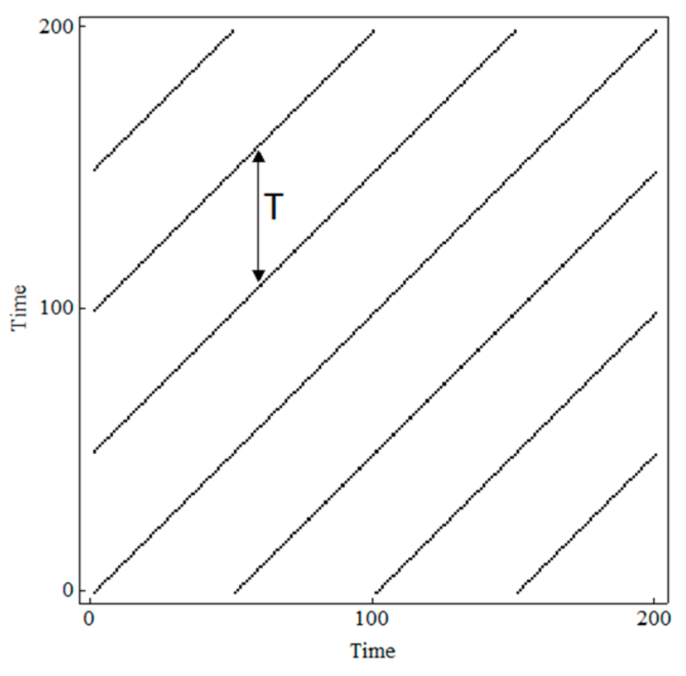
In an RP, a white vertical line between two points provides the recurrence time or Poincaré return time (i.e., the time that it takes for the orbit to return to a previous state). A periodic orbit of period
generates an RP with parallel diagonal lines, all of which are separated by the vertical distance
, as the recurrence occurs at a fixed time interval (
Figure 2). On the other hand, a quasiperiodic orbit provides an RP with parallel diagonal lines, with different distances between them. These distances can be, at most, three different ones, and the largest must be the sum of the other two, in accordance with Slater’s theorem [
16]. RPs of chaotic orbits are quite different however: They show a large number of patterns formed by short diagonal lines and dashed lines and many different return times can be found.
3. Results
This section is organized as follows. In
Section 3.1, we present the phase space of the annular billiard for an ensemble of initial conditions, illustrating the role of the eccentricity
as a control parameter that introduces chaos into the system. We also present plots of a single orbit to illustrate the dynamics of the singular billiard in the limit
. In
Section 3.2, we present the estimations of the largest Lyapunov exponent for some initial conditions for increasing eccentricity
and, therefore, decreasing inner radius
. In this section we present the distribution of the LLEs in the near singular limit as well. Finally, in
Section 3.3, we present RPs of periodic, quasi-periodic and chaotic orbits in the annular billiard and of a typical orbit in the near singular limit. We also discuss the question of sensitive dependence on initial conditions in this limit.
3.1. Phase Space
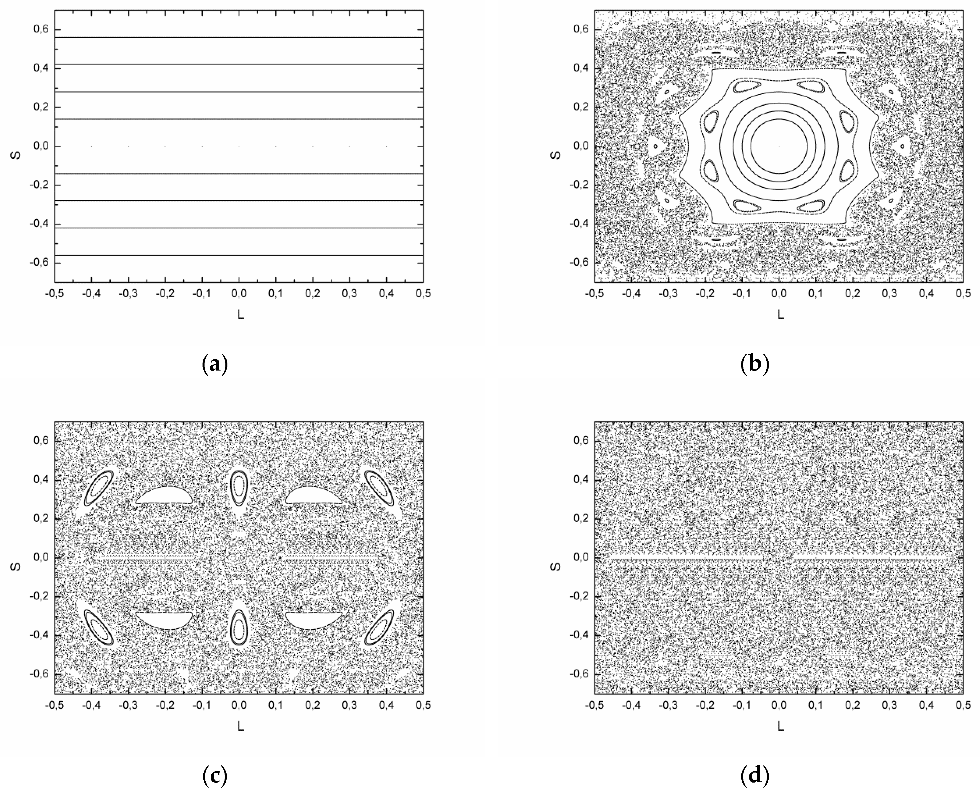
All simulations presented in this section were carried out with in order to keep the regions occupied by the WGO in the Poincaré section constant, i.e., the regions . These regions correspond to straight lines and are omitted in the plots.
The set of plots in
Figure 3 shows the phase space of the annular billiard for different values of eccentricity
. When the boundaries are concentric, i.e.,
, the angular momentum, with respect to the origin of the outer boundary, is preserved, the system is integrable, and the phase space is filled with straight lines parallel to the
-axis. In the eccentric case, i.e.,
, the system is no longer integrable once the angular momentum is no longer a constant of motion, and consequently, structures of resonances and chaos arise. By increasing the value of
the region occupied by the chaotic sea also increases.
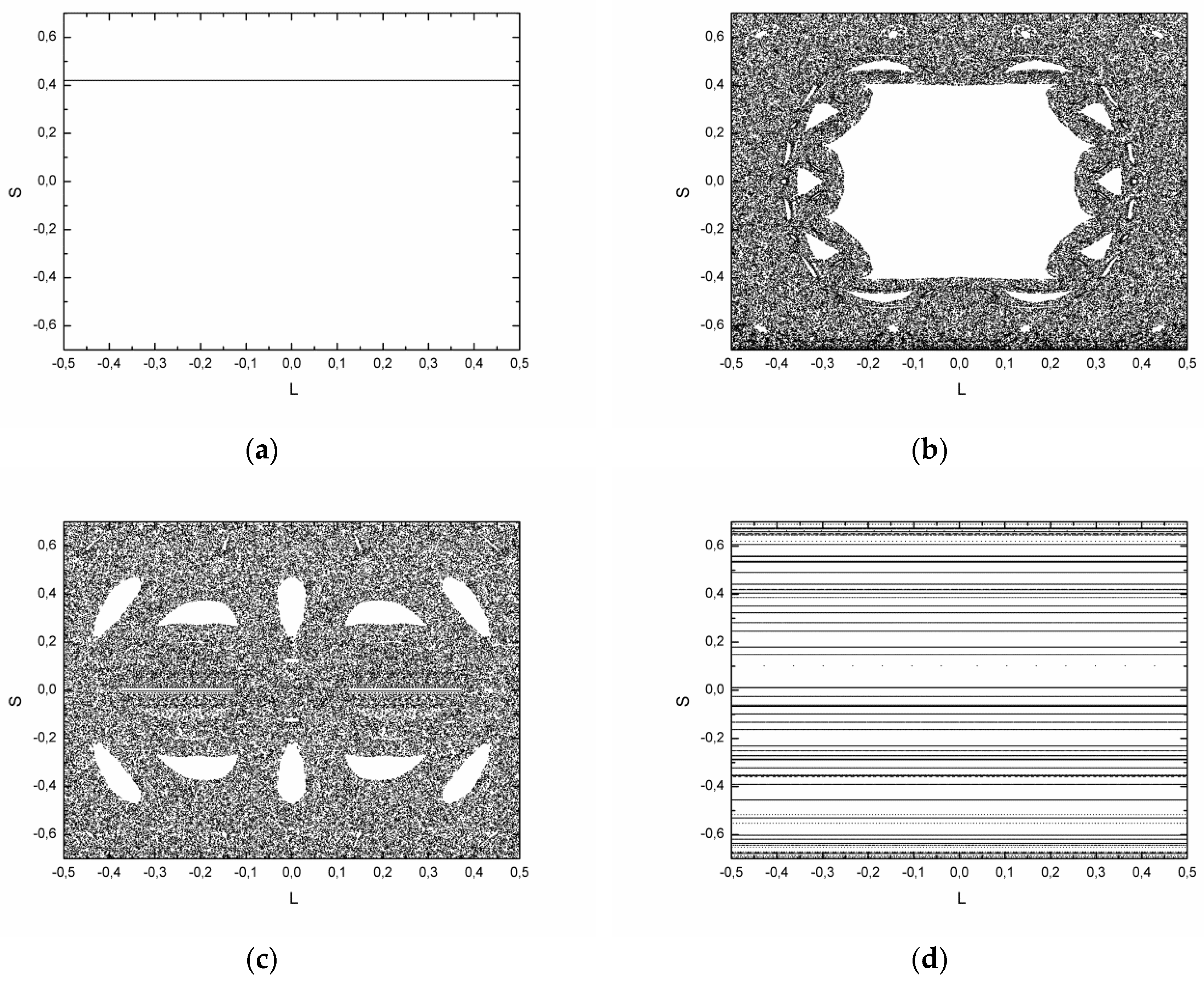
In order to illustrate the dynamics in the singular billiard limit, we will now look at only one orbit in the phase space.
Figure 4 shows the plots of a single orbit, chosen to be in the chaotic sea for the most values of eccentricity, for different values of increasing eccentricity
and, therefore, decreasing inner radius
. In
Figure 4a, we have
, so the system is integrable and the orbit fills a straight line. In
Figure 4b,c, the orbit is chaotic and densely fills the accessible region of the phase space, where the white regions correspond to KAM islands. In
Figure 4d, we have
, so that the radius of the scatterer is four orders of magnitude smaller than the radius of the outer boundary
.
In the near singular limit, a single initial condition fills the phase space with straight lines. This happens because for a given initial condition
the angular momentum of the particle remains constant and equal to
, filling the corresponding straight line (or torus) in the phase space until a collision with the scatterer takes place. When this happens, the angular momentum of the particle is changed, as governed by Equation (3), and another line in the phase space starts to be filled, i.e., another torus is visited. However, once the scatterer is so small, these collisions are rare and the particle spends a long time in the same torus. This process goes on, and by succeeding a sufficiently large number of iterations, the single initial condition densely fills the phase space with straight lines (
Figure 4d).
3.2. Lyapunov Exponent
The largest Lyapunov exponent was calculated with the FTLE method. The finite time chosen was , the interval between rescaling , and the initial distance between the original and the satellite orbits .
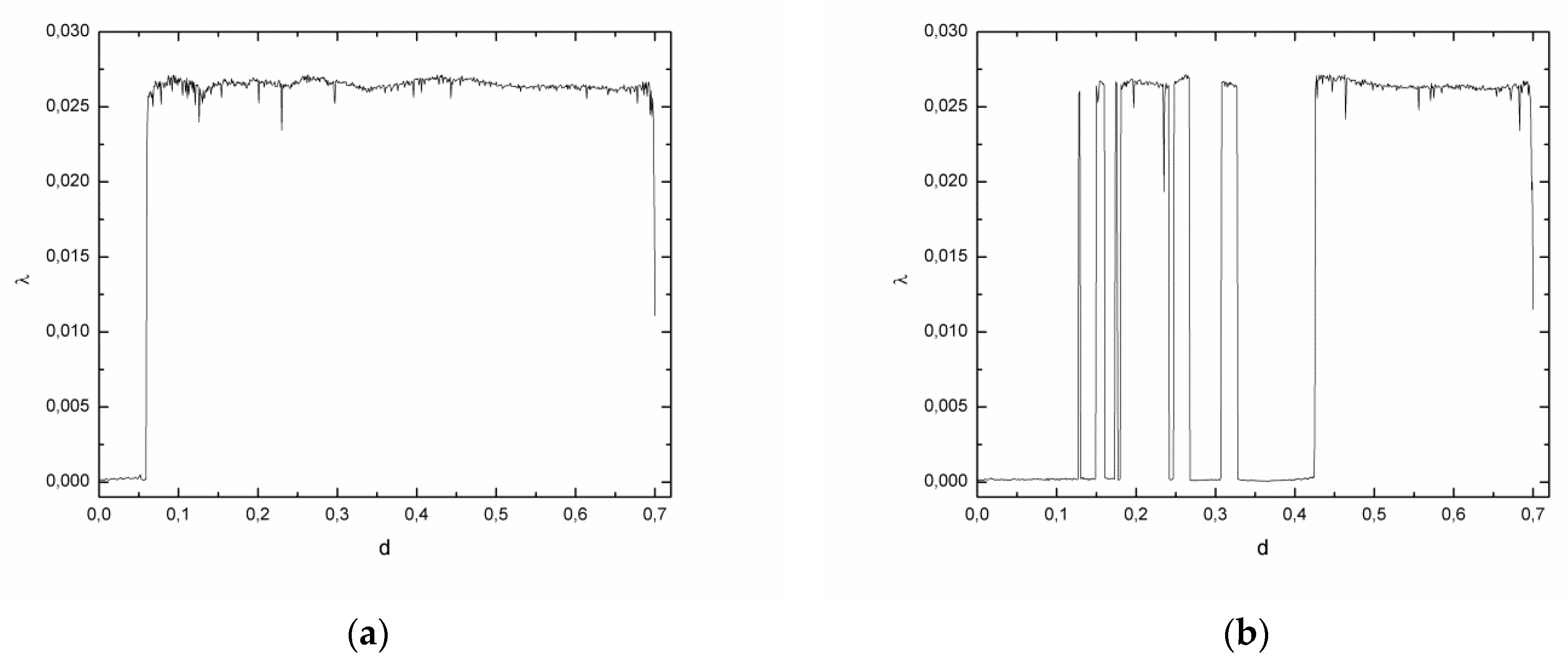
The set of plots in
Figure 5 exhibits values of
as function of the eccentricity
and, therefore, the radius of the scatterer
. For
we have
, corresponding to the near singular limit.
In
Figure 5a, the chosen initial condition was the same as what was used for the plots of
Figure 4, which densely fills the phase space with straight lines in the near singular limit. Initially we have
, and as the eccentricity increases and chaos begins to appear in the system, the Lyapunov exponent becomes positive. The oscillations observed in
are presumably due to stickiness, as KAM islands are created and destroyed as
changes, influencing the behavior of the chaotic orbits. In the near singular limit,
sharply drops for the initial conditions (ICs) in both panels of
Figure 5, evidencing a change in the dynamics of the system. Different initial conditions have been used and this scenario is representative of the near singular case.
In
Figure 5b, we have the IC
, which is not always located in the chaotic sea as the parameter
is varied. There are values of
that give
and this is because the IC is placed at a KAM island for those configurations.
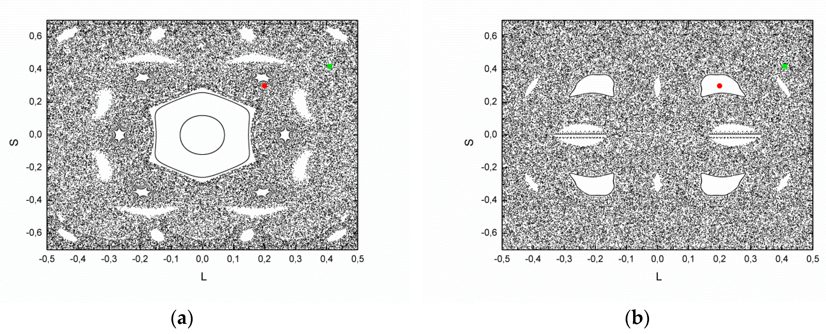
Figure 6 exhibits the phase space for two values of eccentricity, where
in panel (a), for which both ICs of
Figure 5 fall in the chaotic sea and the Lyapunov exponent is positive. In panel (b),
, for which the Lyapunov exponent calculated for the IC of
Figure 5a is positive and for the IC of
Figure 5b, it drops to zero. In both images, the green dot corresponds to the IC of
Figure 5a and the red dot corresponds to the IC of
Figure 5b.
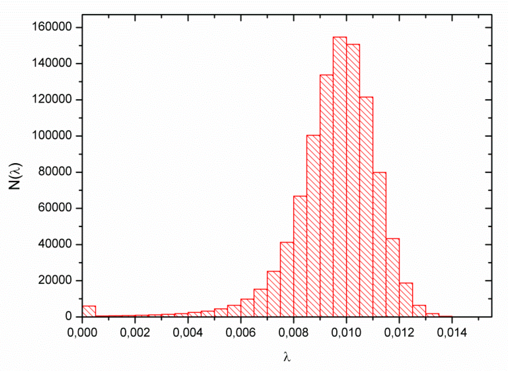
In
Figure 7 we have the distribution of the Lyapunov exponent for 10
6 initial conditions, in the near singular limit, distributed over the
plane region limited by
and
. The Gaussian-like distribution with a tail to the left indicates chaotic dynamics with stickiness. The peak of the distribution is close to the values of λ obtained for the ICs of
Figure 5 in the near singular limit, confirming that these ICs are representative of the dynamics in this limit.
3.3. Recurrence Plots
Each RP presented here was obtained with different values of the threshold , which is the size of the recurrence region. This size has to be evaluated in order to be sure that there are not too few or too many lines in the plots. Although different values of provide different return times for a same orbit, Slater’s theorem is always obeyed in the case of quasi-periodicity.
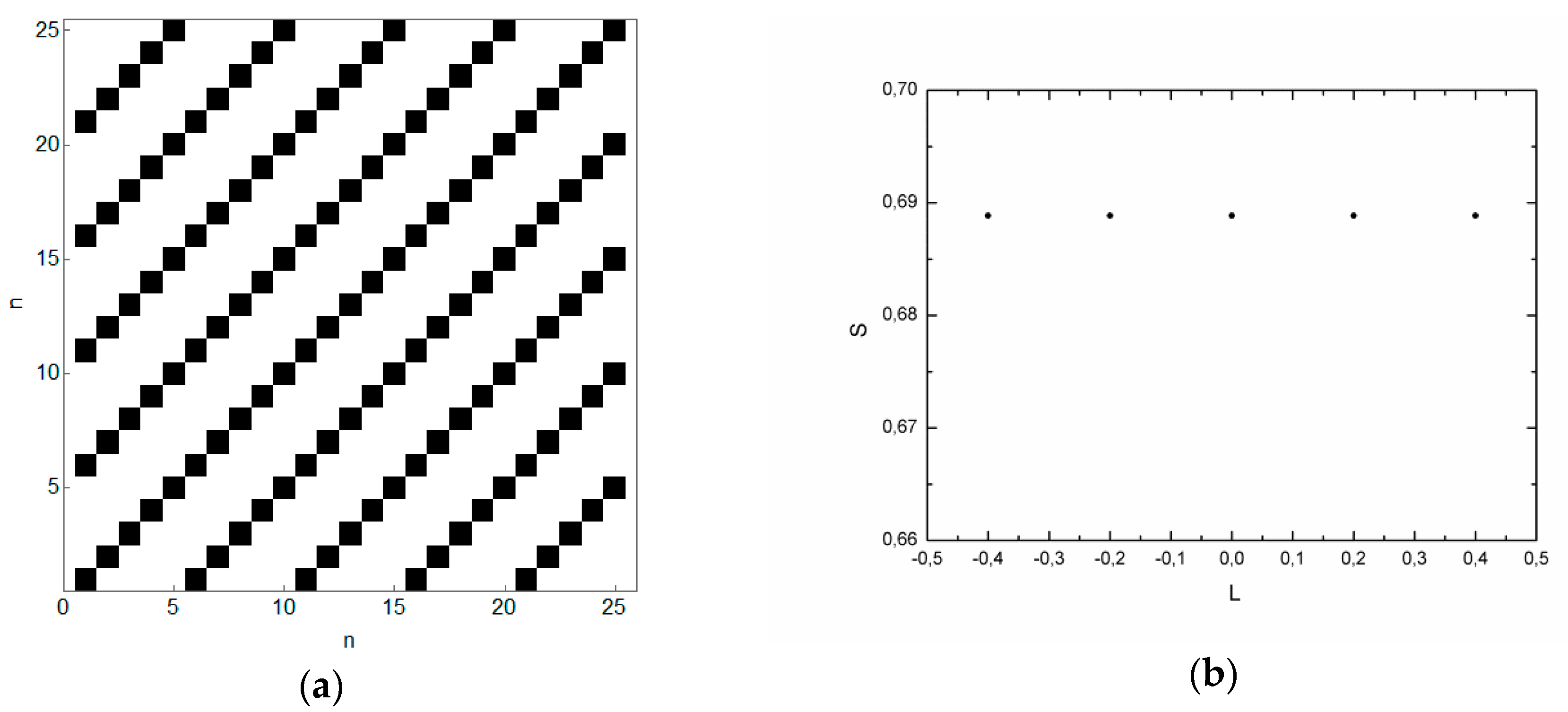
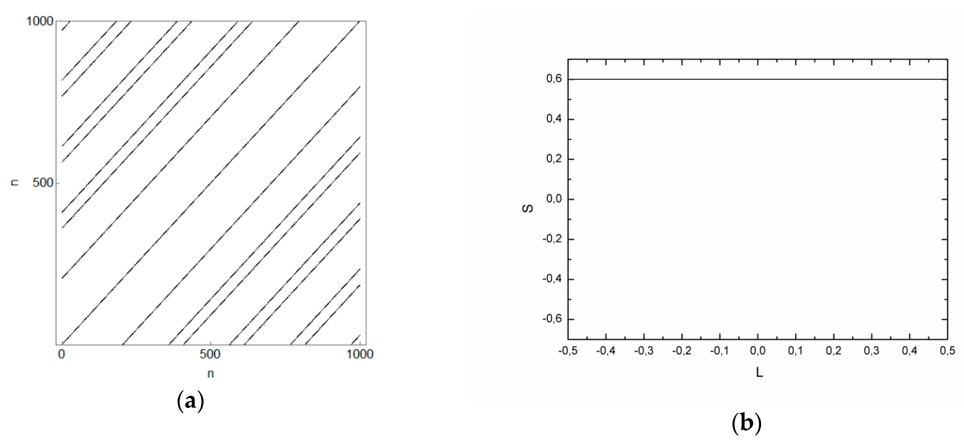
In
Figure 8a, we have the RP of a periodic orbit of period 5 in the concentric annular billiard, obtained with Equation (6), and in
Figure 8b, the same orbit in the phase space. The vertical distance between the lines in the RP of
Figure 8a is always the same and exactly 5, i.e., after five collisions with the outer boundary, the orbit will always return to a previously visited reference state.
Figure 8b shows the same orbit in the phase space, given in the
plane. For the concentric configuration, the angular momentum
of the particle is preserved, so that the orbit remains on the same line (torus) of the
plane. Given the initial condition
, the mapping equations always provide the same five points, as
.
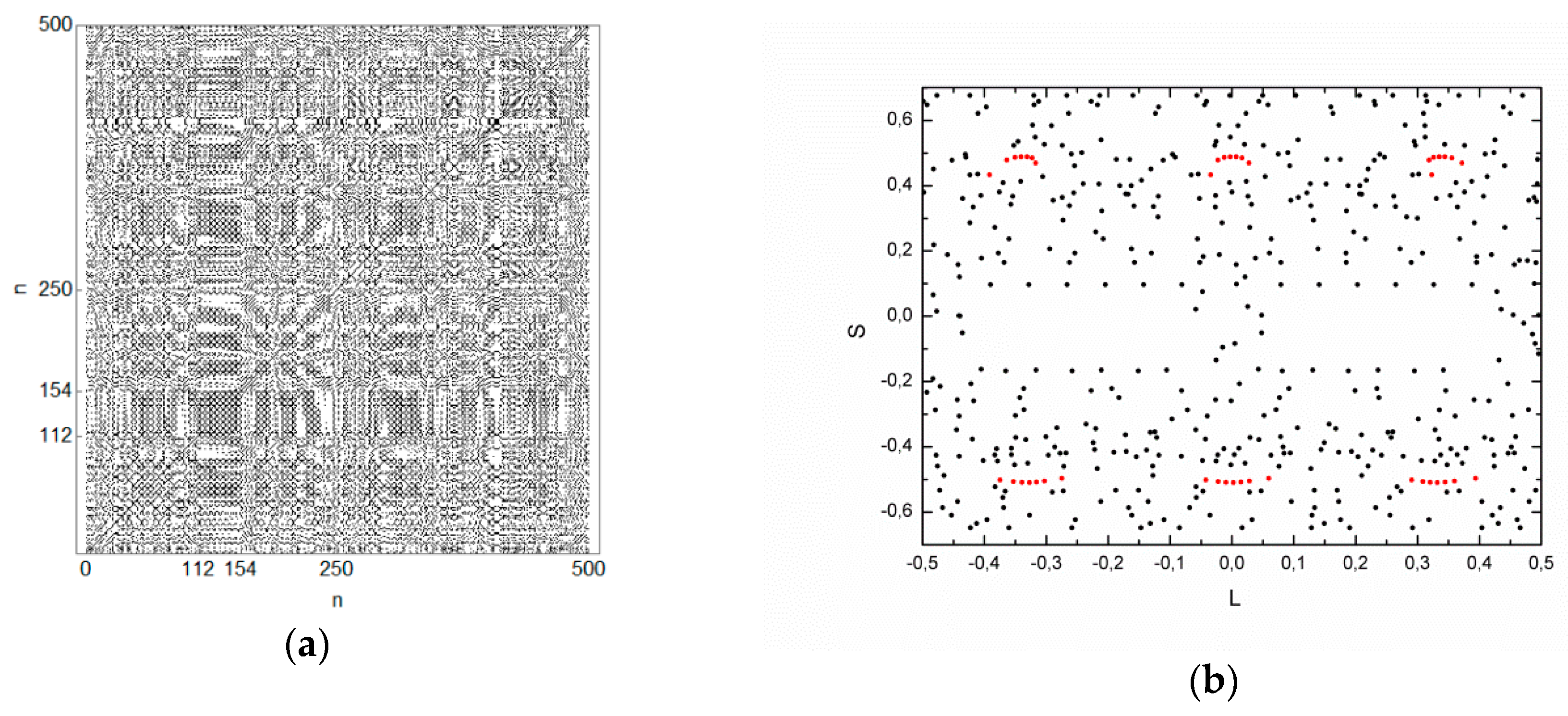
Figure 9a shows an RP of a quasi-periodic orbit and
Figure 9b shows the respective orbit in the phase space. In contrast to the RP of the periodic orbit presented in
Figure 8a, the distances between the diagonal lines of
Figure 9a are not constant, revealing different recurrence times for this orbit.
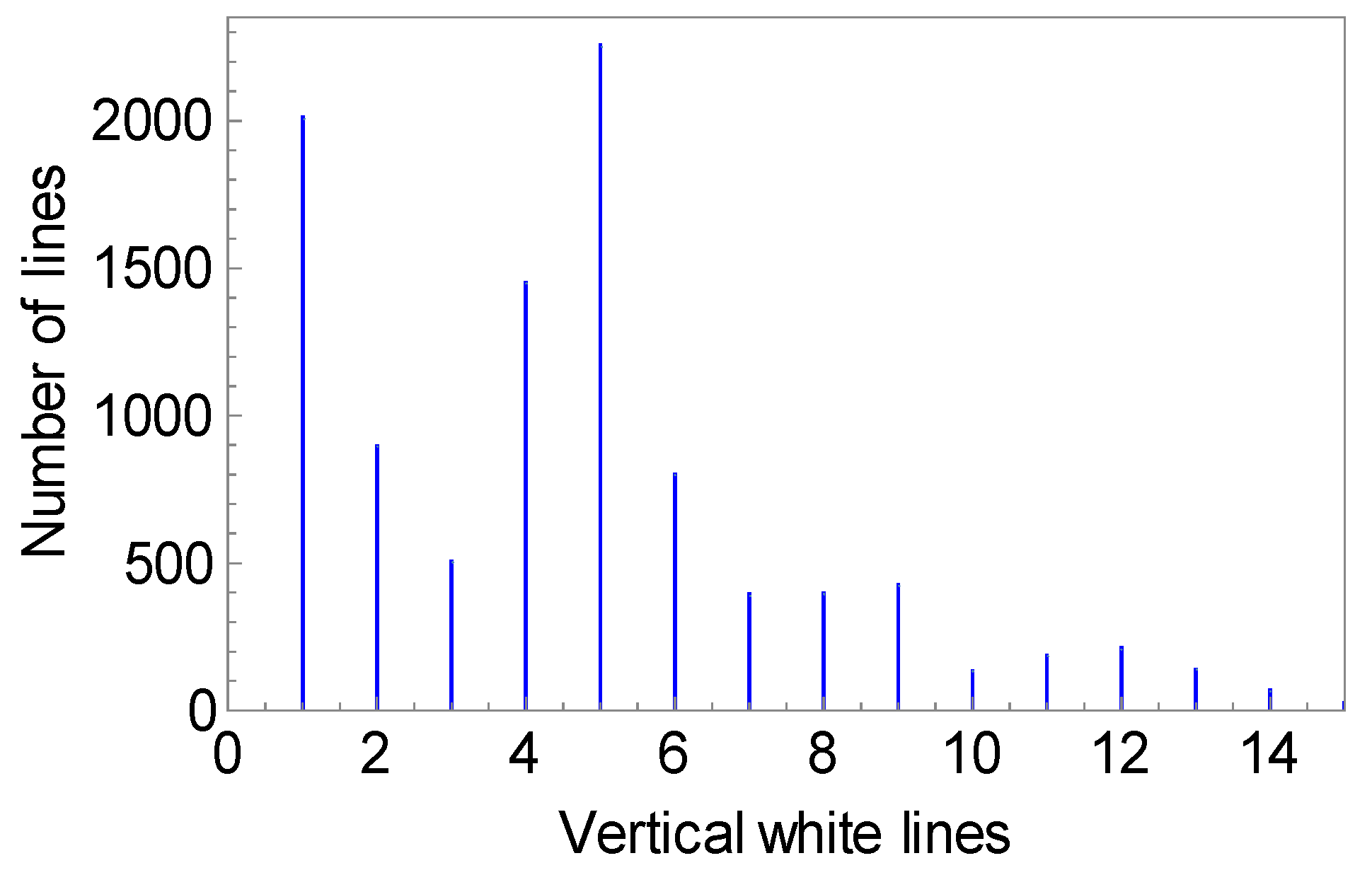
To visualize the recurrence times implicitly shown in the RP, the following numerical procedure was applied to obtain a histogram of vertical white lines. From the recurrence matrix , we first choose , taking the first column of the matrix. Then, we identify the first and second non-zero elements of that column, and , and compute the return time . The next non-zero element, , is found and another return time, , is computed. This process goes on until all the non-zero elements of the first column are considered. The procedure is then repeated for all columns of the matrix. The result can be plotted in a 2D histogram that shows the possible recurrence times as peaks in their respective frequencies of observation.
The histogram in
Figure 10 shows three peaks that correspond to return times equal to
,
and
iterations, and, in accordance with Slater’s theorem,
.
A chaotic orbit of the annular billiard is analyzed in
Figure 10. Differently from the periodic and quasi-periodic cases, the RP of the chaotic orbit (
Figure 11a) shows complex patterns rather than parallel lines. It is possible to observe structures in the diagonal of the RP, as the one found for
. These structures correspond to times when the orbit was trapped by stickiness.
Figure 11b shows the respective orbit in the phase space, where the red dots correspond to the iterations from
to
, when the orbit was suffering stickiness.
The histogram of vertical white lines in
Figure 12 shows that a chaotic orbit has many different return times.
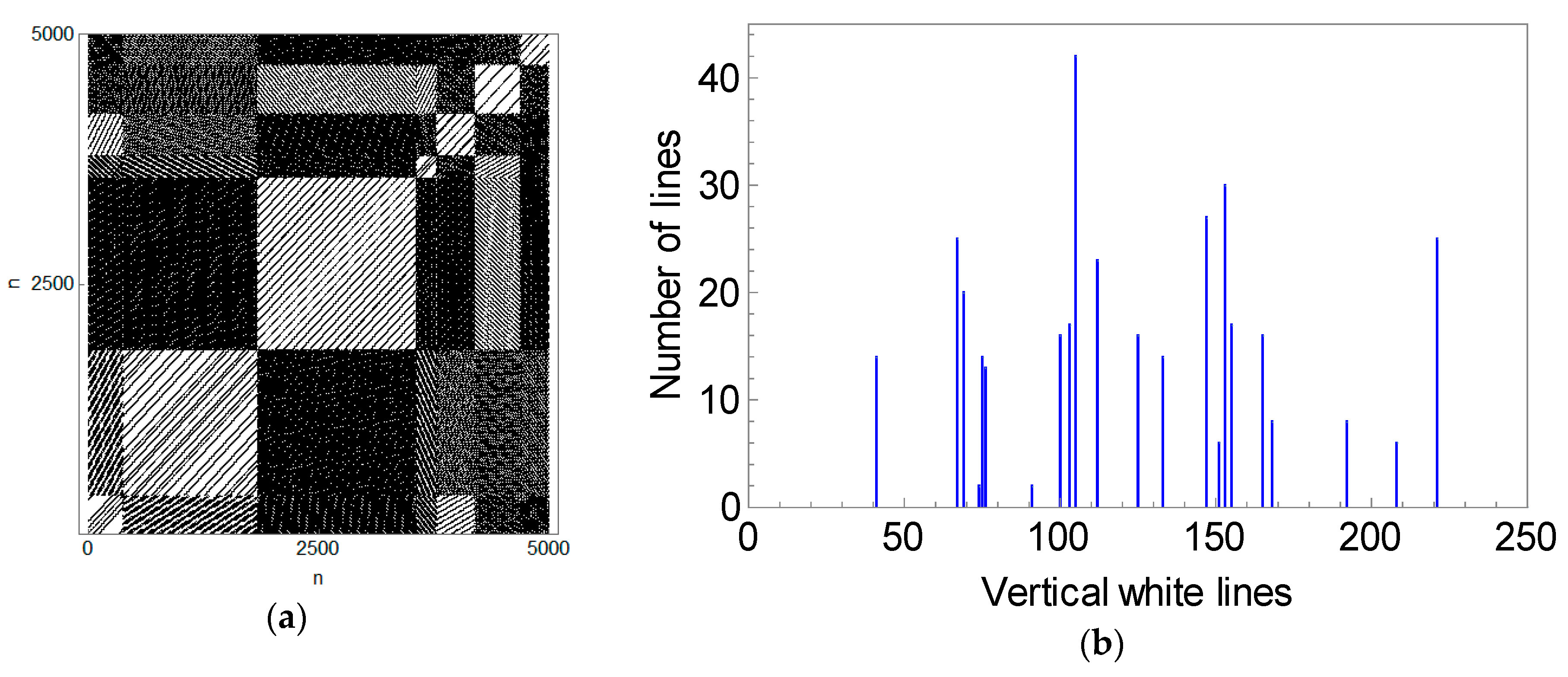
We now analyze the RP of an orbit in the near singular billiard.
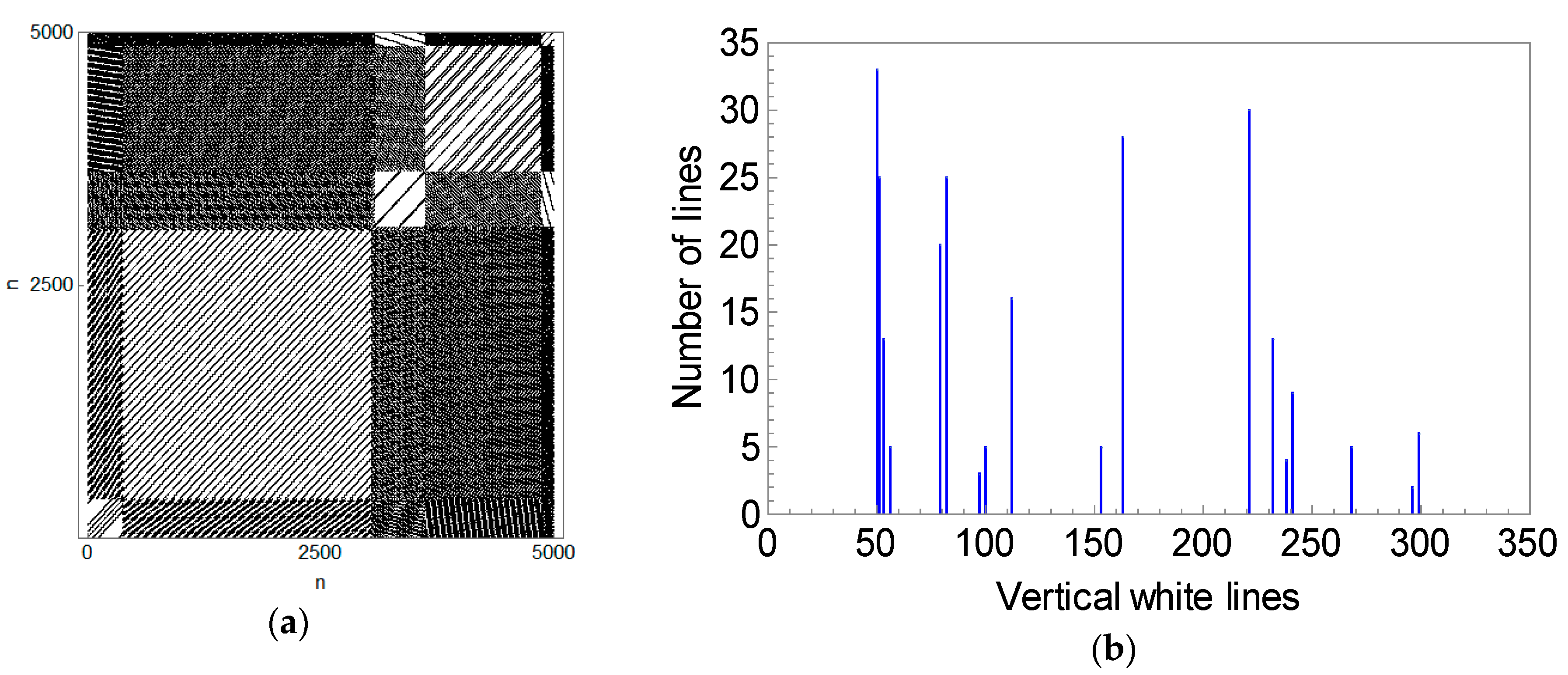
Figure 13 shows the RP corresponding to the orbit of
Figure 4d, which densely fills the phase space with straight lines and the corresponding histogram of vertical white lines. The fact that many different return times are observed states that the orbit is chaotic.
The RP in
Figure 13a is notably different from that of the chaotic orbit in
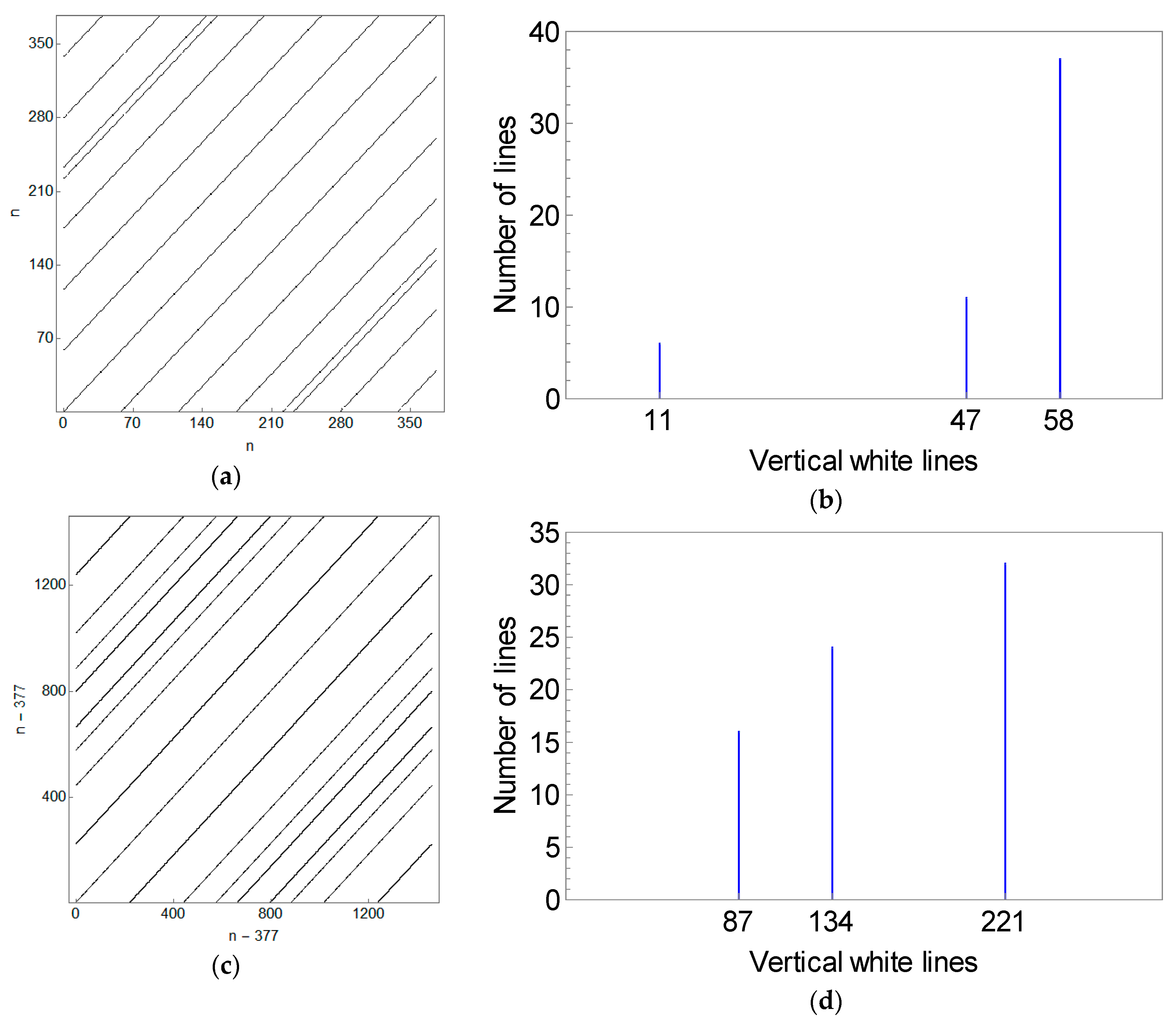
Figure 11a. The orbit in the near singular billiard generates an RP with block-like structures, of straight lines, in a diagonal direction. Separating this RP according to each block (
Figure 14a,c), three return times are observed for each of them and they satisfy Slater’s theorem. It is important to notice that the number of diagonal lines in the RP depends only on the chosen value of
, which is why the RPs of
Figure 14a,c look different than the respective block-like structures of
Figure 13a.
The particle in the near singular billiard behaves quasi-periodically, filling a straight line in the phase space and possessing three return times, until it collides with the scatterer. When this happens, the angular momentum of the particle is changed, another line in the space starts to be filled, and the other three return times are measured on the new torus. The whole phase space is ergodically filled by one single trajectory which has a constant angular momentum between the two collisions with the scatterer. This explains the structures observed in the RP, where the bigger the structure, the longer the time the particle has spent in a given torus.
Sensitivity dependence on initial conditions was also verified for orbits of the near singular billiard. To exemplify this behavior, we set an initial condition in a very close neighborhood of the one used for
Figure 13, in such a way that a distance
initially separates each orbit in the phase space, i.e.,
.
Figure 15a shows the corresponding RP and
Figure 15b shows a histogram of vertical white lines.
The RPs of
Figure 13a and
Figure 15a show the same qualitative properties. Both indicate a chaotic orbit composed of quasi-periodic segments. The difference is in the size of the block-like structures in the diagonals. This is because a small change in the initial condition makes the particle interact with the scatterer at a different time and go to a different torus. The bigger the size of the block-like structure in the RP, the longer the particle has spent in the corresponding torus. Both initial conditions densely fill the phase space with straight lines, but the tori are visited in a different order. Evidently the recurrence times calculated for these two cases also differ, as seen in
Figure 13b and
Figure 15b.


