Structures and Instabilities in Reaction Fronts Separating Fluids of Different Densities

Abstract

Density gradients across reaction fronts propagating vertically can lead to Rayleigh–Taylor instabilities. Reaction fronts can also become unstable due to diffusive instabilities, regardless the presence of a mass density gradient. In this paper, we study the interaction between density driven convection and fronts with diffusive instabilities. We focus in fluids confined in Hele–Shaw cells or porous media, with the hydrodynamics modeled by Brinkman’s equation. The time evolution of the front is described with a Kuramoto–Sivashinsky (KS) equation coupled to the fluid velocity. A linear stability analysis shows a transition to convection that depends on the density differences between reacted and unreacted fluids. A stabilizing density gradient can surpress the effects of diffusive instabilities. The two-dimensional numerical solutions of the nonlinear equations show an increase of speed due to convection. Brinkman’s equation lead to the same results as Darcy’s laws for narrow gap Hele–Shaw cells. For large gaps, modeling the hydrodynamics using Stokes’ flow lead to the same results.

1. Introduction

Reaction fronts propagate in different media separating reactants and products. We find them in systems such as combustion [1,2], directional solidification [3], and waves of chemical activity [4]. In the latter case, a front develops due to the interaction between molecular diffusion and an autocatalytic chemical reaction [5]. Solutions of the reaction-diffusion equations correspond to fronts propagating in a given medium. For thin reaction fronts, these solutions can be approximated by an eikonal relation between the curvature and the normal component of the velocity [6]. The eikonal relation helped to explain the transition to convection for fronts in the iodate-arsenous relation, as well as the change of speed for propagating fronts in a Poiseuille flow [7,8]. Thin fronts showing diffusive instabilities can be modeled using the Kuramoto–Sivashinsky equation, which allows long wavelength instabilities for flat reaction fronts [9]. Experiments taken place in liquids require to take into account fluid motion as an additional component of the front dynamics. Fluid flow can be generated by mass density or surface tension gradients accross the front [10,11,12]. These convective flows will modify the shape of the front, and change its velocity [13,14].

Fronts propagating in the vertical direction can develop diffusive and Rayleigh–Taylor (RT) instabilities in liquids [15,16,17]. While diffusive instabilities are caused by differences in diffusivities, the Rayleigh–Taylor instability will take place if a fluid is placed under another fluid of larger density. Previous work using a reaction-diffusion model coupled to Darcy’s law showed that diffusional instabilities enhance the RT instability, while buoyantly stable configurations can diminish the effects of diffusion-driven instabilities [15,16]. Using the KS equation coupled to Darcy’s law showed the existence of stable cellular structures that involve convection [17]. For fronts propagating in viscous fluids, the KS equation coupled to the Navier–Stokes equation showed oscillatory instabilities depending on the viscosity reflected in a dimensionless Schmidt number [18].

In this paper, we explore the interaction between buoyancy driven flows and diffusive instabilities. Here differences in diffusivities may result in front instabilities even without fluid flow, making it a separate problem from double diffusion convection where buoyancy forces acting on different substances lead to fluid flow. The Kuramoto–Sivashinky equation will model diffusive instabilities in flat reaction fronts when coupled to fluid flow. We consider fluid flows inside Hele–Shaw cells or porous media described by Brinkman’s equation. In a Hele–Shaw cell the fluid is confined between two vertical walls, Brinkmans equation considers the flow only in the direction parallel to the wall, thus becoming in a two-dimensional system. This approximation considers a new term that includes the dimensions of the gap. In the case of narrow gaps, Brinkmans equation can be approximated by Darcy’s law, while for larger gaps the equations become the Navier–Stokes equations. We will carry out a linear stability analysis of the flat convectionless front for perturbations of fixed wavelength. We will also solve numerically the front evolution equations to obtain the patterns appearing in the nonlinear regime.

2. Equations of Motion

Reaction fronts that exhibit diffusive instabilities obey a system of reaction-diffusion equations that allow different diffusion coefficients for each substance. The resulting reaction fronts can be approximated by a front evolution equation, with the position of the front determined by a surface that separates reacted from unreacted species. In a two-dimensional cartesian coordinates ($XZ$) the front can be described by a height function $Z=H(X,t)$, with the time evolution of the height function H determined by a Kuramoto–Sivashinsky (KS) equation coupled to the fluid velocity $\overrightarrow{V}$:

$$\frac{\partial H}{\partial T}=V_0+\mathcal{V}\frac{{\partial }^{2}H}{\partial X^2}+\frac{V_0}{2}{\left(\frac{\partial H}{\partial X}\right)}^2-\mathcal{K}\frac{{\partial }^{4}H}{\partial X^4}+V_z{|}_H.$$

(1)

The parameters $\mathcal{V}$ and $\mathcal{K}$ depend on the diffusion coefficients for the different species. For zero fluid motion, there is a flat front solution that propagates with velocity $V_0$. The stability of this front is determined by the sign of the parameter $\mathcal{V}$. Small perturbations to the flat front of fixed wavelength can growth exponentially if the coefficient $\mathcal{V}$ is negative. This takes place if the wavelength is larger that a critical wavelength, perturbations of smaller wavelenghts will decay. In the opposite case ($\mathcal{V}$ positive), the front is stable regardless the wavelength of the perturbation. In the particular case of a system formed by two species with identical diffusivities involving cubic autocatalysis, the coefficients become $\mathcal{K}=0$ and $\mathcal{V}=D$. In other systems, such as exothermic chemical reactions, the parameters $\mathcal{V}=0$ and $\mathcal{K}$ will depend on the corresponding thermal diffusion coefficient [19,20]. The fluid flow appears as an addition to the normal front velocity of the propagating front [21]. The KS equation involves values up to second order in H, therefore near the onset of convection the normal component of the fluid flow corresponds to the addition of the vertical component of the fluid velocity $V_z$.

In this paper, we consider fluids inside Hele–Shaw cells or porous media, this flow can be described using Brinkman’s equation:

$$\frac{\partial \overrightarrow{V}}{\partial T}+(\overrightarrow{V}·\nabla )\overrightarrow{V}=-\frac{1}{{\rho }_0}\nabla P-12\frac{\nu }{d^2}\overrightarrow{V}+\nu {\nabla }^2\overrightarrow{V}-\frac{\rho }{{\rho }_0}g\widehat{z}.$$

(2)

In this equation P is the pressure, $\overrightarrow{V}$ is the fluid velocity, g is the acceleration of gravity, $\widehat{z}$ is a unit vector pointing upward in the vertical Z-direction, $\nu$ is the coefficient of kinematic viscosity, ${\rho }_0$ is the density of the unreacted fluid, while $\rho$ corresponds to the fluid density that depends on composition of the fluid. In a Hele–Shaw cell, the fluid is confined between two vertical walls separated by a gap width equal to d. For small gap widths, the fluid motion can be modeled with Darcy’s law:

$$\overrightarrow{V}=-\frac{\kappa }{{\rho }_0\nu }(\nabla P+\rho g\widehat{z})P$$

(3)

Here $\kappa$ is the coefficient of permeability for a porous media, which correponds to $d^2/12$ for flows in Hele–Shaw cells. Considering the density differences only in the large gravity term (Bousinesque approximation), the continuity equation is equal to

$$\overrightarrow{\nabla }·\overrightarrow{V}=0.$$

(4)

The continuity equation in two-dimensions allows to derive the fluid velocity from a stream function $\Psi (X,Z,t)$ using the equations $V_x=\partial \Psi /\partial Z$ and $V_z=-\partial \Psi /\partial X$. With these relations we can eliminate the pressure term in Brinkman’s equation to yield

$$\frac{\partial \Omega }{\partial t}=\frac{\partial (\Psi ,\Omega )}{\partial (X,Z)}+\nu {\nabla }^2\Omega -12\frac{\nu }{d^2}\Omega +\frac{g}{{\rho }_0}\frac{\partial \rho }{\partial X}.$$

(5)

The variable $\Omega$ in the last equation is the defined as the vorticity from

$$\Omega ={\nabla }^2\Psi .$$

(6)

We also define the following operator on two given functions F and G:

$$\frac{\partial (F,G)}{\partial (X,Z)}=\frac{\partial F}{\partial X}\frac{\partial G}{\partial Z}-\frac{\partial F}{\partial Z}\frac{\partial G}{\partial X}$$

(7)

The thin reaction front separates fluids of different densities, therefore fluid density can be written as

$$\rho ={\rho }_0+\Delta \rho \Theta (Z-H).$$

(8)

Here $\Theta$ corresponds to the theta function which takes the value of one if the argument is positive, and zero otherwise.

We can reduce the number of parameters under consideration defining appropriate dimensionless units. We introduce time and length scales defined by $L_T=\mathcal{K}/{\mathcal{V}}^2$, and $L_x=\sqrt{(\mathcal{K}/|\mathcal{V}\left|\right)}$. We define $\left|\mathcal{V}\right|$ as unit of the stream function, and $\left|\mathcal{V}\right|/L_x^2$ as unit of the vorticity. The variables in these units will be represented with lower case letters. The dynamic equations become

$$\frac{\partial \omega }{\partial t}=\frac{\partial (\psi ,\omega )}{\partial (x,z)}+{\mathrm{S}}_c{\nabla }^2\omega -\alpha {\mathrm{S}}_c\omega -\mathrm{Ra}{\mathrm{S}}_c\frac{\partial h}{\partial x}\delta (z-h).$$

(9)

This equation involves a dimensionless Rayleigh number

$$\mathrm{Ra}=\frac{g\delta \rho L^3}{\nu \left|\mathcal{V}\right|},$$

(10)

a dimensionless Schmidt number

$${\mathrm{S}}_c=\frac{\nu }{\left|\mathcal{V}\right|},$$

(11)

and a parameter

$$\alpha =\frac{12\mathcal{K}}{d^2\left|\mathcal{V}\right|}.$$

(12)

In this system of units, the KS equation coupled to fluid flow becomes:

$$\frac{\partial h}{\partial t}=c_0-\frac{{\partial }^{2}h}{\partial x^2}+\frac{c_0}{2}{\left(\frac{\partial h}{\partial x}\right)}^2-\frac{{\partial }^{4}h}{\partial x^4}-\frac{\partial \psi }{\partial x}{|}_h,$$

(13)

which involves a dimensionless front speed $c_0$ using the corresponding time and length scales. Reactions taking place in aqueous solutions have a large Schmidt number, therefore we will consider this limiting case where Equation (9) becomes

$${\nabla }^2\omega -\alpha \omega -\mathrm{Ra}\frac{\partial h}{\partial x}\delta (z-h)=0.$$

(14)

2.1. Linear Stability Analysis

The equations describing the evolution of the system (Equations (1) and (2)) allow a flat front solution moving with constant velocity $c_0$. We introduce perturbations of wavenumber q to this solution of the form

$$\psi =\widehat{\psi }\left(z\right)e^{\sigma t}sin\left(qx\right)$$

(15)

and

$$h=h_1{e}^{\sigma t}cos\left(qx\right)$$

(16)

leading to

$${(\frac{d^2}{d{z}^2}-q^2)}^2\widehat{\psi }-\alpha \omega +\mathrm{Ra}q{h}_1\delta \left(z\right)=0$$

(17)

and

$$\sigma h_1=(q^2-q^4)h_1-q\widehat{\psi }\left(0\right).$$

(18)

The strategy for solving this system consists in first solving the linear equation Equation (17) in terms of $h_1$ and then substituting into Equation (18). The delta function leads to the following jump conditions at $z=0$:

$$[\widehat{\psi }]=[\frac{d\widehat{\psi }}{dz}]=[\frac{d^2\widehat{\psi }}{d{z}^2}]=0\mathrm{and}[\frac{d^3\widehat{\psi }}{d{z}^3}]=-\mathrm{Ra}q{h}_1.$$

(19)

$$(k^2-q^2)(k^2-\alpha -q^2)=0.$$

(20)

From here we obtain four values for k, namely $\pm q$, and $\pm k_{\alpha }$, where $k_{\alpha }=\sqrt{q^2+\alpha }$. Considering that the stream function should vanish as the absolute value of the coordinate z becomes large, it lead us to write

$${\psi }_1\left(z\right)=\left\{\begin{array}{cc}A{e}^{-qz}+B{e}^{-k_{\alpha }}\hfill & \mathrm{if} z\ge 0\hfill \\ C{e}^{qz}+D{e}^{k_{\alpha }}\hfill & \mathrm{if} z<0\hfill \end{array}\right.,$$

(21)

Applying this for the stream function on the jump conditions across the front, we find a system of linear equations

$$\begin{array}{cc}\hfill A+B-C-D& =0\end{array}$$

(22)

$$\begin{array}{cc}\hfill qA+k_{\alpha }B+qC+k_{\alpha }D& =0\end{array}$$

(23)

$$\begin{array}{cc}\hfill q^{2}A+k_{\alpha }^{2}B-q^{2}C-k_{\alpha }^{2}D& =0\end{array}$$

(24)

$$\begin{array}{cc}\hfill q^{3}A+k_{\alpha }^{3}B+q^{3}C+k_{\alpha }^{3}D& =\mathrm{Ra}q{h}_1\end{array}$$

(25)

The solution of this system determines the stream function given a particular value of $h_1$, therefore

$$\widehat{\psi }\left(0\right)=A+B=-\frac{\mathrm{Ra}{h}_{1}q}{2k_{\alpha }q(q+k_{\alpha })}$$

Thus we obtain a dispersion relation between the growth rate $\sigma$ and the wavenumber q which depends on the Rayleigh number and the parameter $\alpha$ which incorporates the gap width d on the model.

$$\sigma =q^2-q^4+\frac{\mathrm{Ra}{q}^2}{2k_{\alpha }q(q+k_{\alpha })}.$$

(26)

2.2. Numerical Solutions

We use numerial methods to look for complex solutions of the nonlinear KS equation coupled to convective fluid motion. This solutions can be found in regimes where the flat front is unstable. Since the fluid flow is considered near the onset of convection, only linear terms for the velocity field are kept. To simplify further the problem allowing a direct comparison with Darcy’s law limit, fluid boundary conditions are taken as slip-free boundaries. Therefore we can use a Fourier expansion on the front and stream function:

$$\psi =\sum _{n=1}{\psi }_n(z,t)sin\left(nqx\right),$$

(27)

and

$$h=\sum _{n=0}{H}_n\left(t\right)cos\left(nqx\right).$$

(28)

Here the domain varies from $x=0$ to $x=L$ with the parameter q being equal to $\pi /L$. This expansion also incorporates the appropriate boundary conditions for h, which corresponds to vanishing first and third derivatives at the walls. Substituting into the linearized equation for the stream function allows to solve each Fourier coefficient in terms of the functions $H_n\left(t\right)$. This solution is similar to the one carried out in the linear stability analysis, therefore the KS equation with this solution becomes:

$$\frac{\partial h}{\partial t}=c_0-\frac{{\partial }^{2}h}{\partial x^2}+\frac{c_0}{2}{\left(\frac{\partial h}{\partial x}\right)}^2-\frac{{\partial }^{4}h}{\partial x^4}+\sum _n\frac{\mathrm{Ra}nq{H}_n}{2nq{k}_n(nq+k_n)}$$

(29)

The value of variable $k_n$ is defined by $k_n=\sqrt{{\left(nq\right)}^2+\alpha }$. Introducing the expansion on the nonlinear KS equation results in a set of coupled ordinary differential equations for the coefficients $H_n$

$$\frac{d{H}_0}{dt}=c_0+c_0\frac{q^2}{4}\sum _p{p}^2{H}_p^2$$

(30)

$$\begin{array}{c}\frac{d{H}_n}{dt}=[{\left(nq\right)}^2-{\left(nq\right)}^4+\frac{\mathrm{Ra}{\left(nq\right)}^2}{2k_{n}nq(nq+k_n)}]H_n+\hfill \\ c_0\frac{q^2}{4}\sum _{l,p}lp{H}_p{H}_l\times ({\delta }_{n,|l-p|}-{\delta }_{n,l+p}),\mathrm{for}n\ge 1.\hfill \end{array}$$

(31)

In this work, we study the stability of convectionless flat front solutions (determined by Equation (26)), and steady curved fronts involving convection. To this end, we only consider the first 16 terms of Equation (31) setting the time derivatives equal to zero. The resulting nonlinear system was solved numerically using the scipy library from python through the module optimize.fsolve. Higher order truncations did not change the front solutions significantly. Each steady front solution has a constant velocity $c=d{H}_0/dt$ calculated using Equation (30). 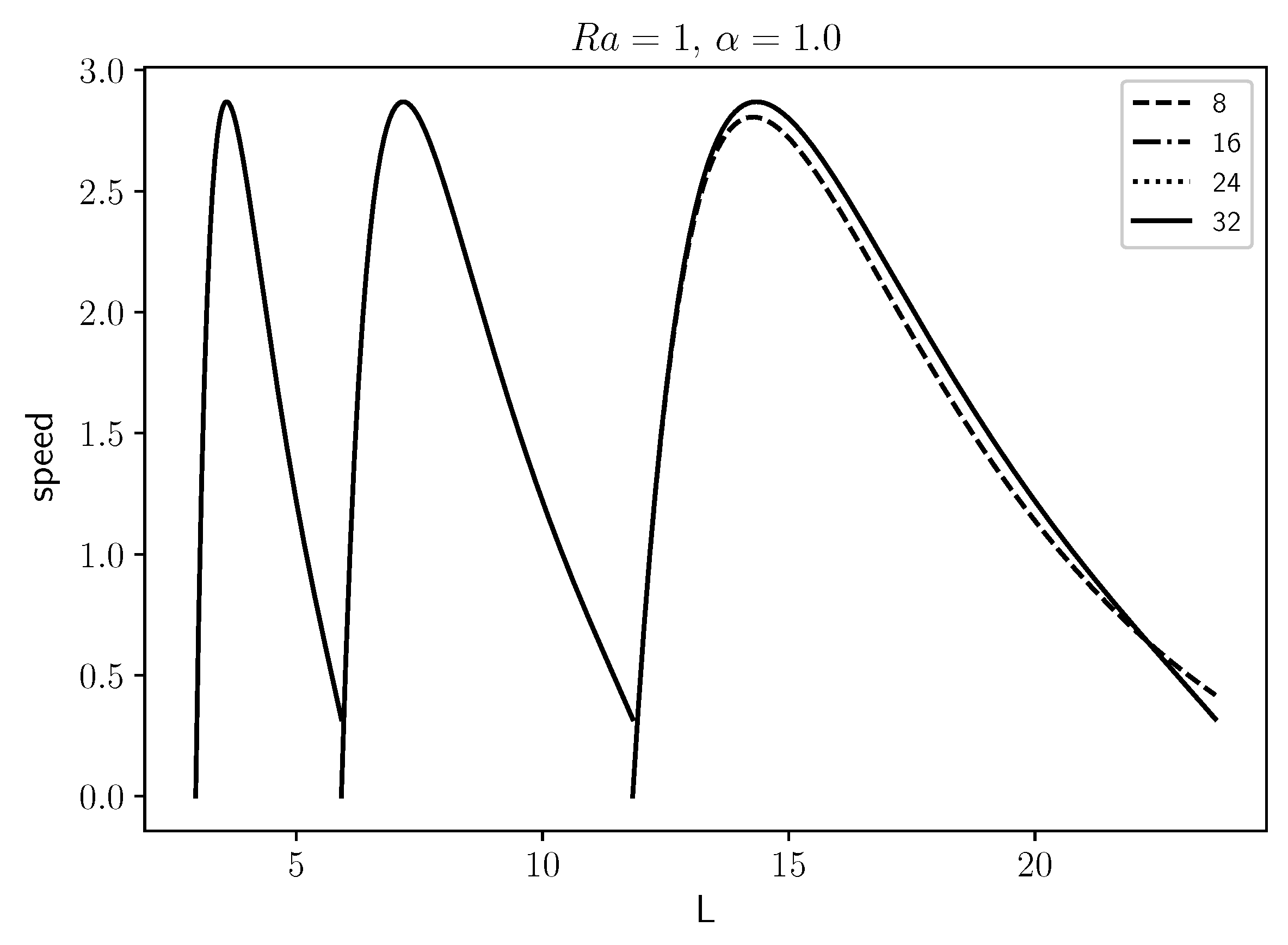To address the issue of convergence, we displayed in Figure 1 the front speed relative to the flat front speed using an 8, 16, 24, and 32 terms truncation showing that the last three are indistinguishable from each other.

We obtained solutions for different values of the parameters $\alpha$, $Ra$, and L analyzing their stability, considering the flat front speed $c_0=1$. To determine the front stability, we used Python routines to obtain the eigenvalues of the Jacobian matrix derived from Equation (31). The sign of the largest real part of the eigenvalues determines the stability of the steady front, a negative sign will indicate stability. We also study solutions that evolve in time (such as oscillatory or chaotic solutions) using a simple Euler method to evolve Equation (31) with a time step $\Delta t={10}^{-3}$, and 18 term truncation.

3. Results

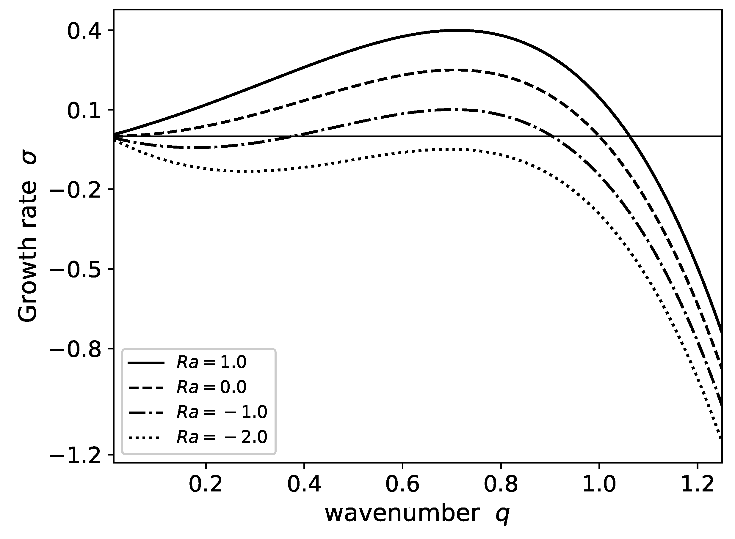
The density discontinuity accross the reaction front either enhances or inhibits the flat front instability found in the KS equation. Without fluid flow ($\mathrm{Ra}=0$), the dispersion relation Equation (26) has positive growth rates for perturbations of large wavelengths (small wavenumbers q) as shown in Figure 2. In this case perturbations of wavenumbers smaller than a critical value $q_c=1$ have positive growth rates, indicating a flat front instability. In the case of positive Rayleigh numbers, where the less dense fluid is under a heavier fluid, the situation is similar. There is a critical wavenumber where perturbations with smaller wavenumber will grow, however this value is greater than one, the critical value without fluid flow. Therefore positive Rayleigh numbers will enhance the flat front instability. The opposite situation is found for negative Rayleigh numbers. Here the range of wavenumbers that allow negative growth rates diminishes. As we decrease the Rayleigh number from zero, the wavenumbers that lead to instabilities correspond to an interval that does not start in zero. That is near $q=0$, the perturbations have negative growth rate, turning into positive growth rates as we increase q, and then becoming negative once again as we increase q further. This interval diminishes, and finally disappears, as we decrease the Rayleigh number towards negative values. Therefore, for a given negative value of the Rayleigh number the flat front becomes stable. A large enough density gradient is able to stabilize the flat fronts described by the KS equation.

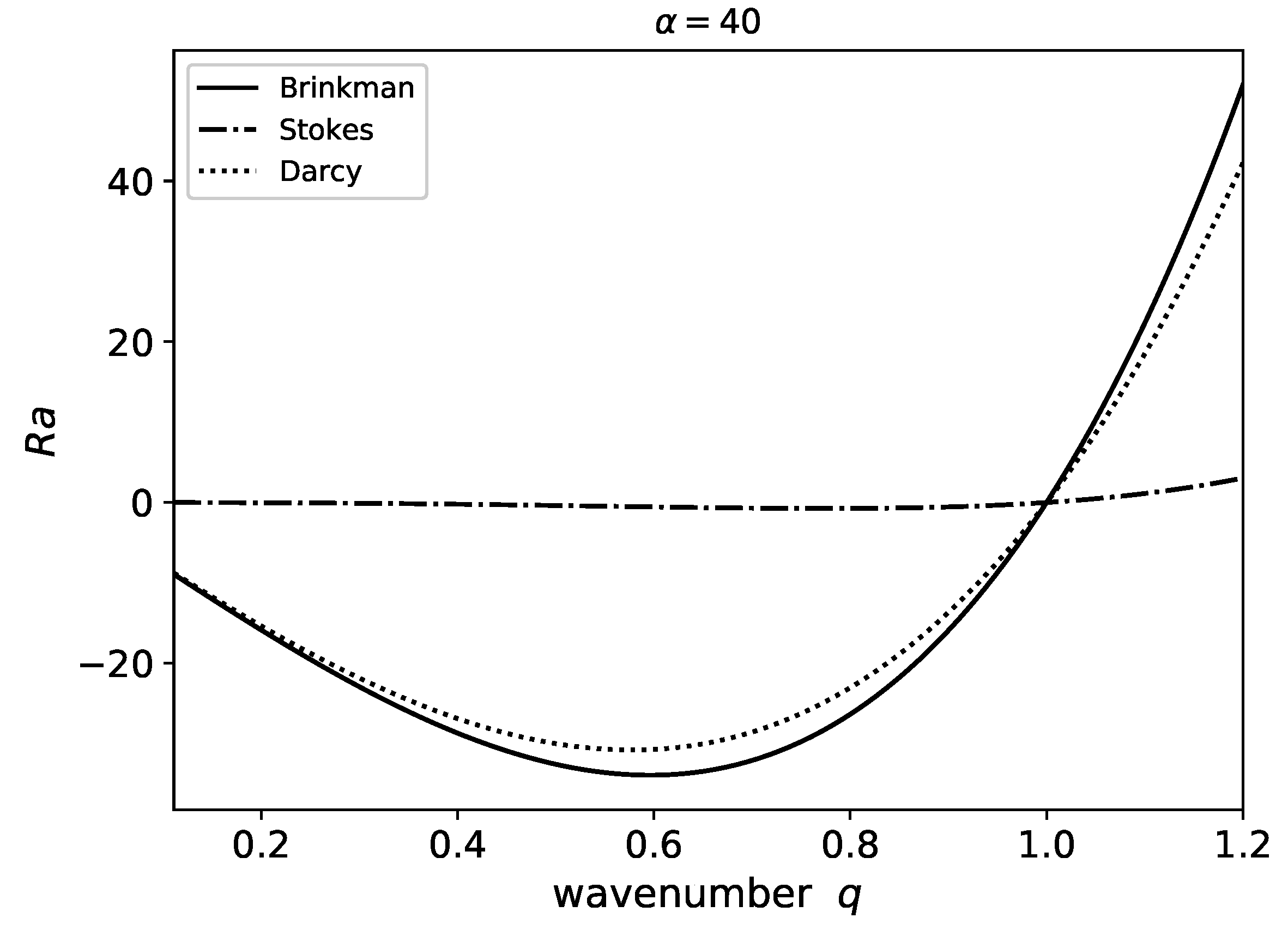
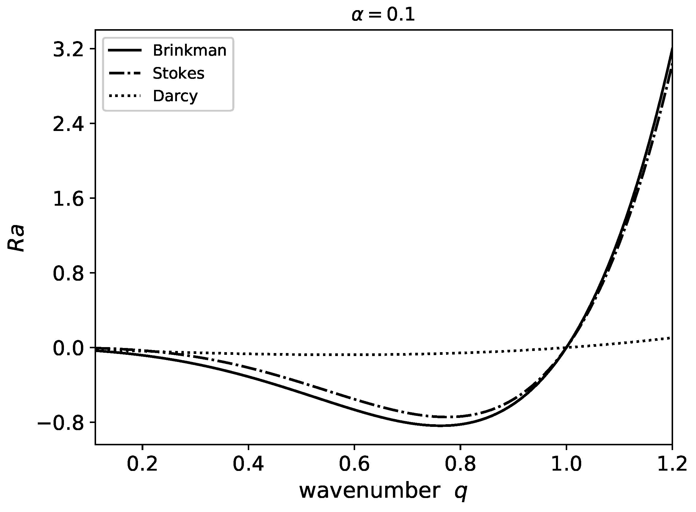
Perturbations of fixed wavenumber can be stabilized with an appropriate Rayleigh number. Figure 3 shows the Rayleigh number necessary for growth rate equal to zero for different values of the wavenumber q.

In this figure, we compare three hydrodynamic models including Brinkman’s equation. The curve for the Brinkman’s model has a minimum, therefore a stable flat front requires a Rayleigh number below the minimum. This curve also shows that perturbations with wavenumber below 1 require a negative Rayleigh number to avoid a growing perturbation. For Rayleigh numbers that are negative but above the minimum, there is an interval in the values of q with positive growth rates. In these cases the front can be stable for long wavelength perturbations (small values of q). In Figure 3 we also display the results using two other hydrodynamic models: Darcy’s law and the Stokes equation. In a Hele–Shaw cell width a narrow gap (as is the case for $\alpha =40$), the results of Darcy’s law are close to the results using Brinkman’s equation. Flows in Hele–Shaw cells with narrow gaps can be described with Darcy’s law, which is the limiting case of Brinkman’s equation. With a wider gap ($\alpha =0.1$), we find that the results using the Stokes equation are closer to the results of Brinkman’s equation (Figure 4), approaching the correct wide gap limit. Brinkman’s equation provide us the results between the two limits.

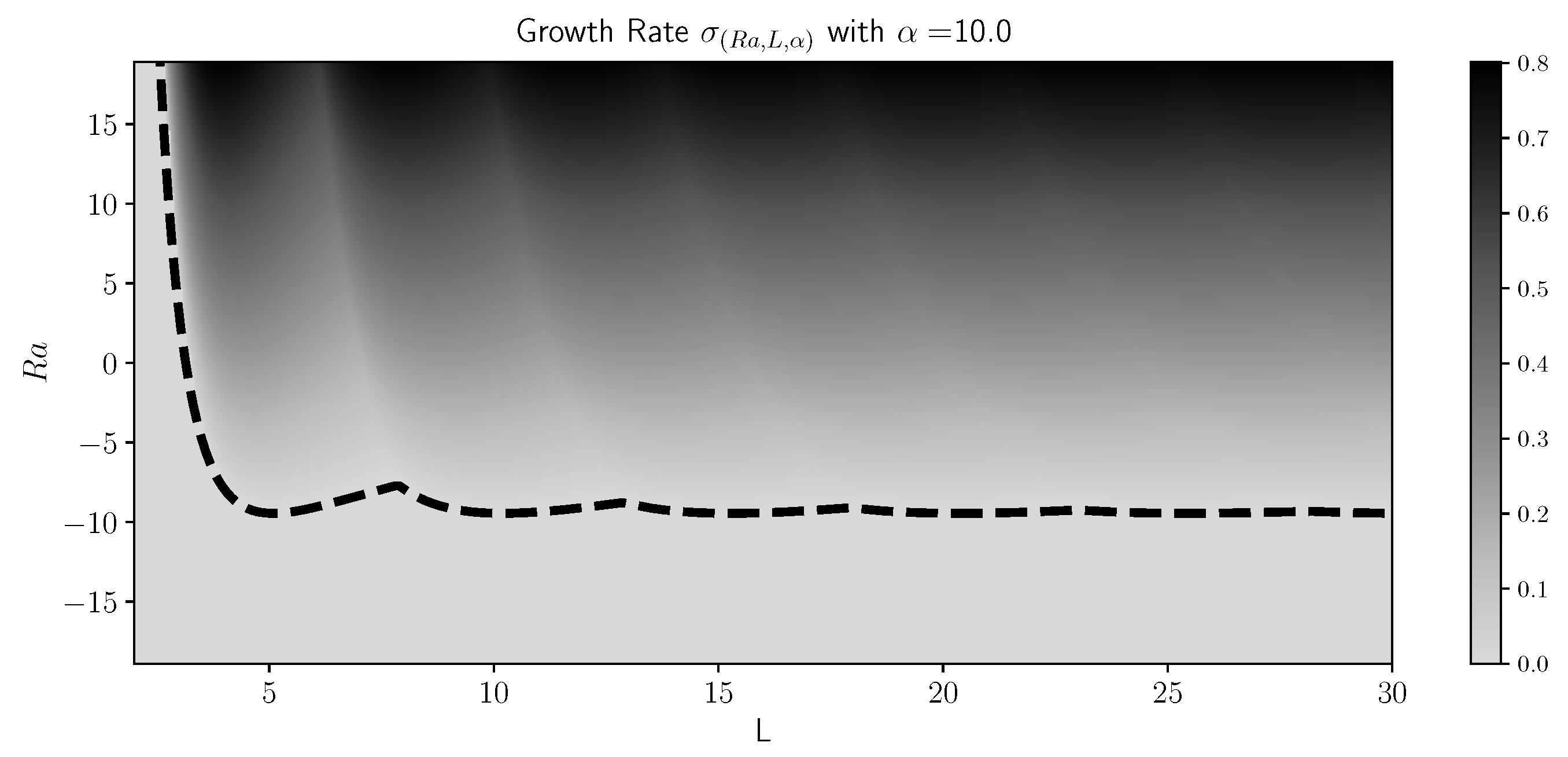
Flat fronts propagating in two-dimensional rectangular domains (resembling vertical tubes), can be stable depending on the value of the Rayleigh number. Figure 5 displays the largest growth rate as a function of Rayleigh number and domain width. A solid curve separates the regions of positive and negative growth rate, consequently values under the curve indicate a stable flat front. Narrow rectangular domains of width equal to L allow only perturbations of wavenumber greater than $q=\pi /L$. Since perturbations of $q<1$ require positive Rayleigh numbers to generate instabilities, domains with $L<\pi$ will require a less dense fluid is under a more dense fluid to trigger an instability. On the contrary, if $L>\pi$, the flat front requires a negative Rayleigh number to be stable. We observe in Figure 5 that the critical Rayleigh number for front instability fluctuates as a function of the domain width. This implies that a flat front can be unstable for a certain width, but increasing the width could stabilize the flat front, if the original Rayleigh number is now below the new critical value.

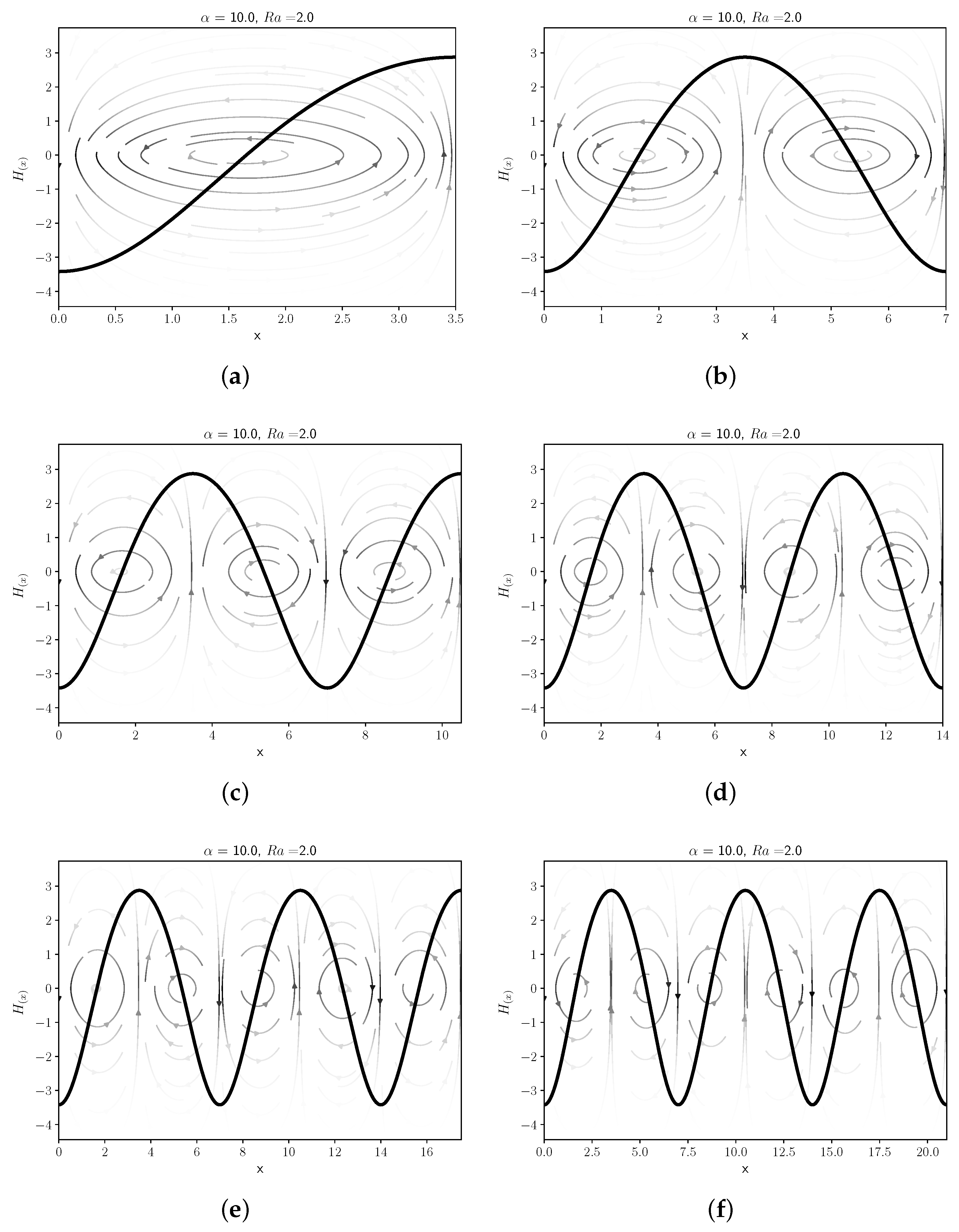
Increasing the domain size beyond the critical value for the flat front instability leads to convective fluid motion. Numerical solutions of the nonlinear equations just above criticality show that small random perturbations to the flat front grow with time. After some time, they form a steady pattern with fluid rising on one side of the domain and falling on the opposite side generating a single convective roll as shown in Figure 6a. The mirrored solution is also a steady solution of the equation, that developes from different initial conditions, and is also stable. The patterns propagate with constant shape and a velocity higher than the velocity for the flat front. This shape also leads to steady front solutions for rectangular domains of larger widths. For example, doubling the domain size we can accomodate two single counterrotating convective rolls as shown in Figure 6b. These solutions have the same speed as the single roll solution, but in this case the fluid rises at the center of the rectangular domain falling on the sides. The resulting shape corresponds to a symmetric front with a maximum near the center of the domain. We can continue this process for larger domains, finding structures formed by placing a one roll solution, next to another counterrotating one roll solution. The first structures formed in this manner are displayed in Figure 6. The solutions with an even number of convective rolls are symmetric with respect to the center of the domain. The mirrored solution is also a solution, for the case of fronts with odd number of rolls. This solution resemble the cellular solutions found in the Kuramoto–Sivashinky equation [20]. We will analyze later the conditions for stabily of the cellular solutions.

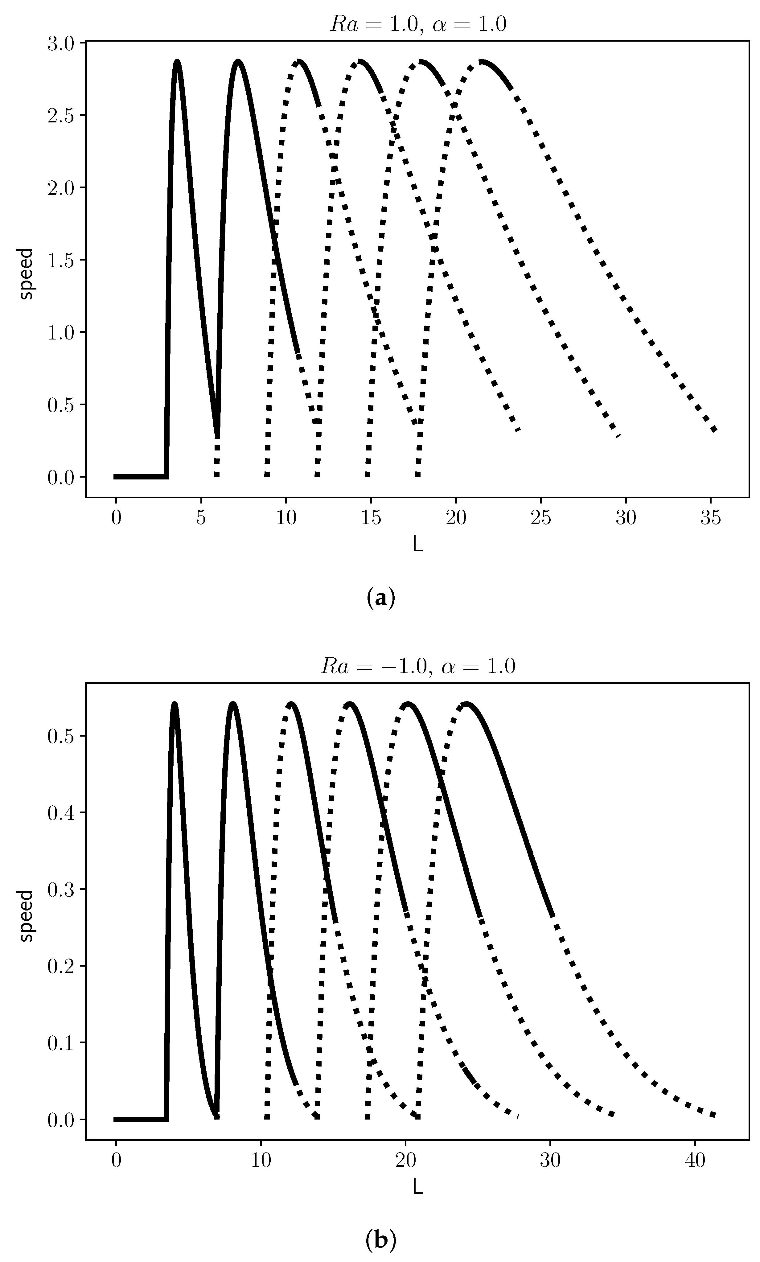
Convection increases the speed of propagating fronts as they propagate upward in narrow vertical rectangles. Progating fronts of steady shape develop when the width of the tube is larger than a critical width. In Figure 7a we display the speed of fronts relative to the flat front speed ($c-c_0$) as a function of the domain width for a positive Rayleigh number ($\mathrm{Ra}=1$). Below the critical width, the only solution corresponds to the flat front solution. As we increase the width above the critical width the solution with one convective roll appears. The analytical linear stability analysis shows that the flat front is unstable beyond the critical width. The linear stability analysis of the curved fronts were carried out obtaining the Jacobian matrix on the steady solutions of Equation (31) as described in Section 2.2.

This linear stability analysis determines that the single roll solution is stable for widths above, but close, to the critical width. Increasing the width further also increases the speed of the convective front until it reaches a maximum value. After the maximum value is reached, the front speed decreases until the one roll solution is not available, at this point there is another solution containing two counterrotating convective rolls. The linear stability analysis shows that the one-roll solution is always stable. There is a small range of values that allows both the one-roll, and the two-roll solution, in this case one the one-roll solution is stable. Once the one-roll solution is no longer available, the two-roll solution appears, increasing the speed as the width is increased, reaching a maximum, and finally disappearing. However, contrary to the one-roll solution, the two roll solution is not always stable, there are regions of instability. Figure 7 also displays the speed relative to the flat front speed of steady solutions with three, four, and five rolls. In all these cases, the behavior is similar, the speed increases, reaches a maximum, after that decreases, and then the solution is no longer available. However in all these cases, the solution is unstable for most values, only for small ranges the solution is stable. For negative values of the Rayleigh number ($\mathrm{Ra}<0$), the critical width for convective fronts decreases (Figure 7b). The speed of the cellular structures have a similiar behavior as for positive Rayleigh numbers, that is they show width values where the solution exist, achieving a maximum speed for certain widths. However, in this case the speeds are lower, but the width values showing stable fronts is larger. Having the less dense fluid above the more dense fluid contributes to stabilize structures, but with a corresponding decrease in velocity. 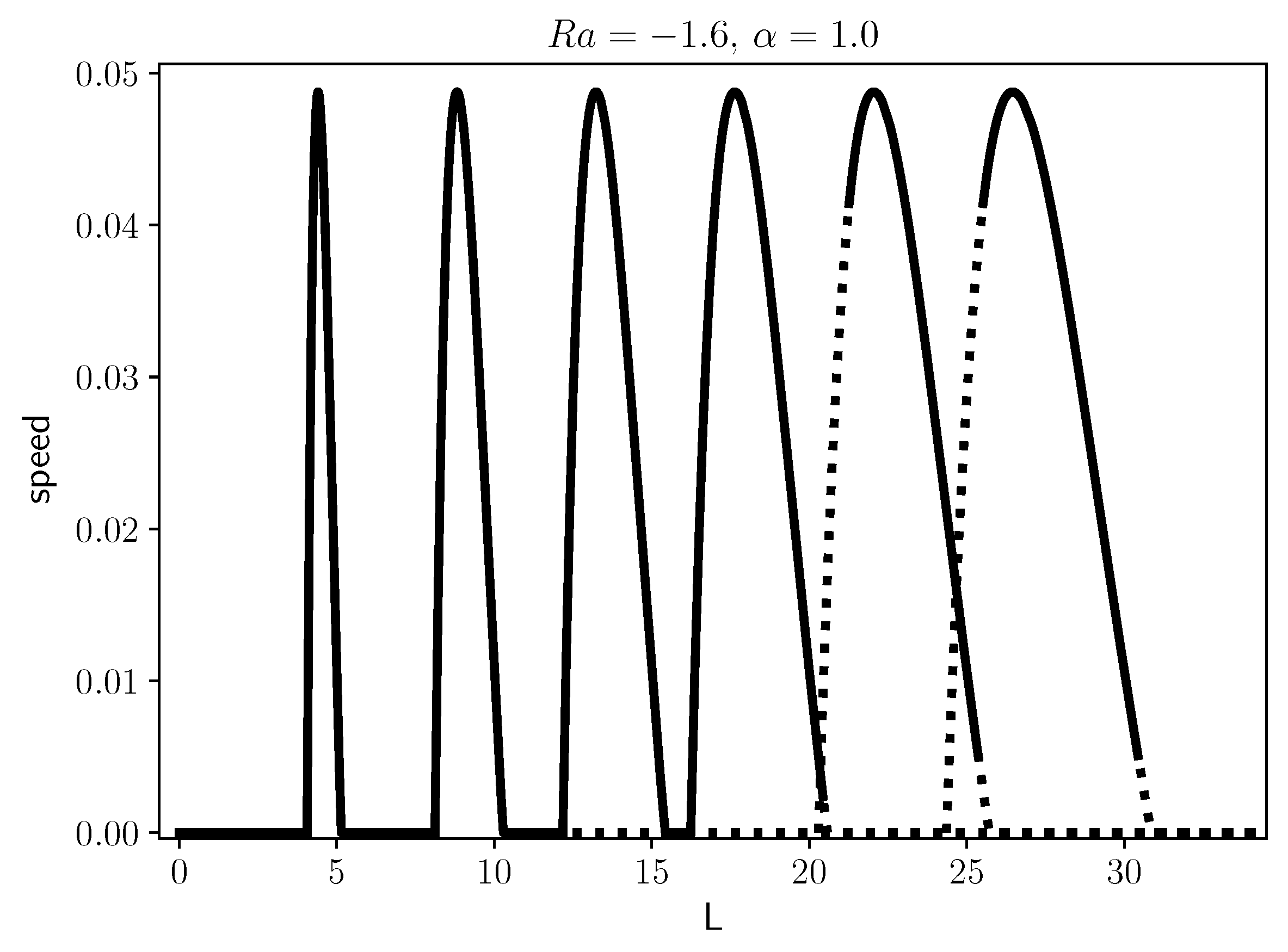Lowering the Rayleigh number to $\mathrm{Ra}=-1.6$ we find even lower convective front velocities relative to the flat front speed (Figure 8). In this case increasing the width leads to a region where the convective solution is no longer possible, where the flat front is stable once again. Increasing the width will lead to effectively stopping convection.

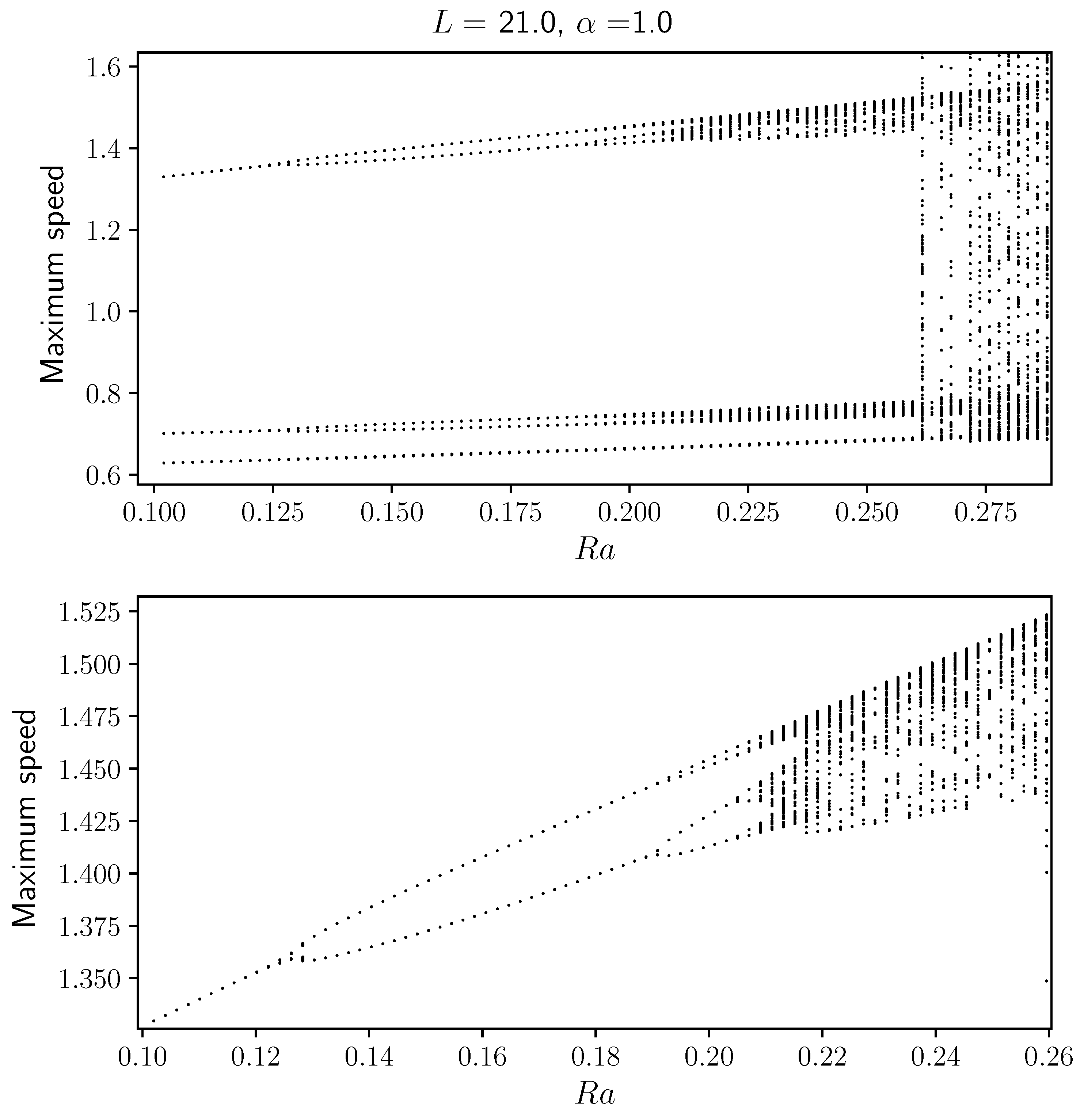
Fronts described by the KS equation exhibit complex spatio-temporal behavior, such as oscillations and chaos. Fluid motion and confinement can help to enhance or surpress this behavior. In Figure 9 we display a bifurcation diagram showing the relative maximum front speed relative to the flat front speed as a function of the Rayleigh number. As the front evolves with time its propagating velocity changes, reaching a maximum before slowing down. Oscillatory fronts will display a few maxima before repeating the sequence again. For values of the Rayleigh number close to $\mathrm{Ra}=0.1$, Figure 9 displays three velocity maxima. As the Rayleigh number increases, we observe a sequence of bifurcations to oscillatory states with higher periodicity. This period doubling cascade leading to chaotic states is the result of enhanced fluid motion at higher Rayleigh numbers. Negative Rayleigh numbers inhibit the oscillatory motion resulting in flat front thus surpressing complex fluid motion. Another parameter that has an impact on complex behavior is the parameter $\alpha$, which is inversely proportional to the square of the gap width. Figure 10 shows a similar period doubling cascade displaying the front velocity maxima relative to the flat front speed versus the parameter $\alpha$. We notice that for $\alpha$ close to 1.34 there is clearly periodic behavior. Reducing $\alpha$ increases the number of maxima, eventually reaching a chaotic state. This implies that confining the substances in a Hele–Shaw cell of small gap (large $\alpha$) diminish the complex spatio-temporal behavior. This implies that in experiments in a Hele–Shaw cell, the gap width can be an effective control parameter for transitions between different spatio-temporal states.

4. Summary and Discussion

We found that the presence of density gradients in fronts governed by the KS equation could enhance or supress complex behavior. Positive density gradients ($\mathrm{Ra}>0$) lowers the critical wavelength for onset of convection, thus fronts propagating in rectangular domains would require smaller widths for flat front stability. On the contrary, negative Rayleigh numbers provide a mechanism to diminish the instability found in the KS equation. Fronts propagating with parameters just above the flat front instability evolve into a curved front of constant shape involving a single convective roll. Placing this single roll solution (or cell) next to each other results in cellular structures that are extended solutions on a larger domain. We analyzed the stability of these structures as a function of the domain widths finding corresponding regions of stability. A density gradient favorable to convection diminishes the widths for stability, on the other hand, a gradient unfavorable to convection increases the stability of cellular structures. Decreasing the negative Rayleigh number even further leads to a situation where unstable flat fronts can be stabilized by increasing the width of the domain. We also found that complex behavior can be surpressed by either reducing the Rayleigh number, or by controlling the gap width in Hele–Shaw cells. The latter being a mechanism that can useful to experiments. A connection with experiments will require knowledge of the parameters $\mathcal{V}$ and $\mathcal{K}$. An estimate can be obtained by using the wavelength for maximum growth rate for purely diffusive instabilities, which in dimensioned units corresponds to $\lambda =2\pi /q=2\pi \sqrt{2\mathcal{K}/\mathcal{V}}$. A second relation between $\mathcal{V}$ and $\mathcal{V}$ can be obtained from the experimental front speed $V_0$, which in dimensionlesss units correspond to $c_0=V_0{L}_T/L_x=1$. Using these relations as a guide, we can compute the value of the Rayleigh number using $\mathrm{Ra}=g\delta {\lambda }^2/8{\pi }^2\nu c_0$. We can use a typical wavelength of about 1 cm observed in experiments [22] together with parameters from chemical reaction fronts propagating in aqueous solutions [7] obtaining a Rayleigh number of $-45$, where the more dense fluid is above the fluid of smaller density. This Rayleigh number requires a value of $\alpha =53.8$ to inhibit the diffusive instability, which leads to a distance between plates in a Hele–Shaw cell equal to 0.5 mm. This distance is small, but larger gaps can be used if the absolute value of the Rayleigh number can be diminished. Therefore experiments can be carried out for different gap values of Hele–Shaw cells to test how the density differences between reacted and unreacted fluids can supress the diffusive instability. One of the advantage of using Brinkman’s equation in the calculations is that it leads to the correct narrow and wide gap limits, which are governed by Darcy’s law and the Navier–Stokes equations.