An Analytical Study of Adversely Affecting Radiation and Temperature Parameters on a Magnetohydrodynamic Elasto-viscous Fluid

Abstract

An investigation of how the velocity of elasto-viscous fluid past an infinite plate, with slip and variable temperature, is influenced by combined thermal-radiative diffusion effects has been carried out. The study of dynamics of a flow model leads to the generation of characteristic fluid parameters ($G_r$, $G_m$, M, F, $S_c$ and $P_r$). The interaction of these parameters with elasto-viscous parameter $K^{{}^{\prime }}$ is probed to describe how certain parametric range and conditions could be pre-decided to enhance the flow speed past a channel. In particular, the flow dynamics’ alteration in correspondence to the slip parameter’s choice, along with temperature provision to the boundary in temporal pattern, is determined through uniquely calculated exact expressions of velocity, temperature and mass concentration of the fluid. The complex multi-parametric model has been analytically solved using the Laplace and Inverse Laplace transform. Through study of calculated exact expressions, an identification of variables, adversely (M, F, $S_c$ and $P_r$) and favourably ($G_r$ and $G_m$) affecting the flow speed and temperature has been made. The accuracy of our results have also been tested by computing matching numerical solutions and by graphical reasoning. The verification of existing results of Newtonian fluid with varying boundary condition of velocity and temperature has also been completed, affirming the veracity of present results.

1. Introduction

Biochemical radiative processing in treatment of several diseases, filtration processes of complex nature with narrow gateways and nuclear reactor processes [1,2,3,4,5,6], involve the phenomenon of varying-degree of mass-heat diffusion. This process of combined radiative-mass flow is also observed in metal-cooling in reactors and industrial processes on the macro-level. The overlapping nature of heat and mass conduction process for smaller concentration gradient differences has led researchers to study heat-mass transfer phenomenon in convective flows simultaneously [7,8,9,10,11,12,13,14,15,16,17]. Moreover, the study of electrically conducting fluids (Magnetohydrodynamic fluids, MHD) has been necessitated to understand many industrial and physical processes such as checking the magnetic control in iron flow [18,19,20], etc.

Consolidated results representing the study of Newtonian and non-Newtonian fluid systems along with radiative heat and mass transfer have been accumulated [21,22,23,24]. Several aspects of dynamics of flow like variations caused by boundary condition on velocity, shear stress and mixed boundary conditions have been discussed in [25,26,27,28]. Flow past a vertical oscillating channel was first mathematically described in [29] and investigation of convective flow dynamics was further carried out to include mass transfer phenomenon [30]. Some interesting results regarding the probe of convective flows with constant heat flux provided by boundary of channel and effects of transverse magnetic field on fluid motion [31,32] were presented. How altering degree of radiation and temperature provision impacted flow dynamics along with properties of flow in porous medium were discussed by [33,34]. More recently, flow speed enhancing factors like induced shear on channel boundary was discussed in [35,36], through calculation of closed form solutions using fractional derivatives. Keeping the nature of polymeric fluids with memory effects in mind, the investigation of related fluid dynamics using slip boundary condition is considered to be imperative and has been discussed in our present article.

To understand the mechanism of multi-faceted applications in aerospace engineering and bioengineering, efforts have been employed to study the characteristics of elasto-viscous fluid system. The development of such a fluid system is deemed important as its features add into the interesting angle of probe into boundary layer control problems as well as it helps to reflect on excretory organ mechanism. Though the dynamics of elasto-viscous fluids have been studied recently but complexity of highly non-linear equations with the combination of characteristic fluid parameters tend to present difficulty in calculating exact solutions. A numerical solutions’ approach has been adopted to develop the models of convective heat-mass transfer of elasto-viscous fluids past or over straight channels that were moved impulsively or started with constant and uniform acceleration [37,38]. These observations also included the angle of normal oscillations of channel and adjacent convection. In an ionized flow system, electromagnetic diffusion was probed by [39,40]. Some efforts were dedicated to analyse MHD nano-fluid dynamics system with induction of high temperature insulation and heat radiation in porous mediums [5,11,41,42,43]. Some of elasto-viscous fluids overlap in the category of fluids having changing viscosity. Thus, presenting the need of such models to be investigated [44] on thorough basis.

However, in all the works above, either numerical solutions were sought for elasto-viscous fluids model along with no-slip condition on boundary or exact solutions for comparatively simpler flow models were determined by employing velocity, shear stress and mixed conditions on boundary. In our present work, we have analysed the heat and mass transfer of convective flow of elasto-viscous fluid with slip boundary condition such that provision of temporal temperature on the boundary of infinite plate over which fluid is flowing is ensured. Unlike the usual numerical approach towards determining such complex models ’ solutions, we have obtained exact closed form solutions. It has been probed that how elasto-viscous parameter, K impacts the flow speed in combination with characteristic fluid parameters $G_r$, $G_m$, $P_r$, M, F and $S_c$. An interesting conclusion about a particular strength of slip parameter and the manner with which infinite plate boundary is provided the temperature has been reached to optimize the flow speed. The present results of elasto-viscous fluid system have also been verified through graphical approach as well as by considering limiting cases of fluid parameters.

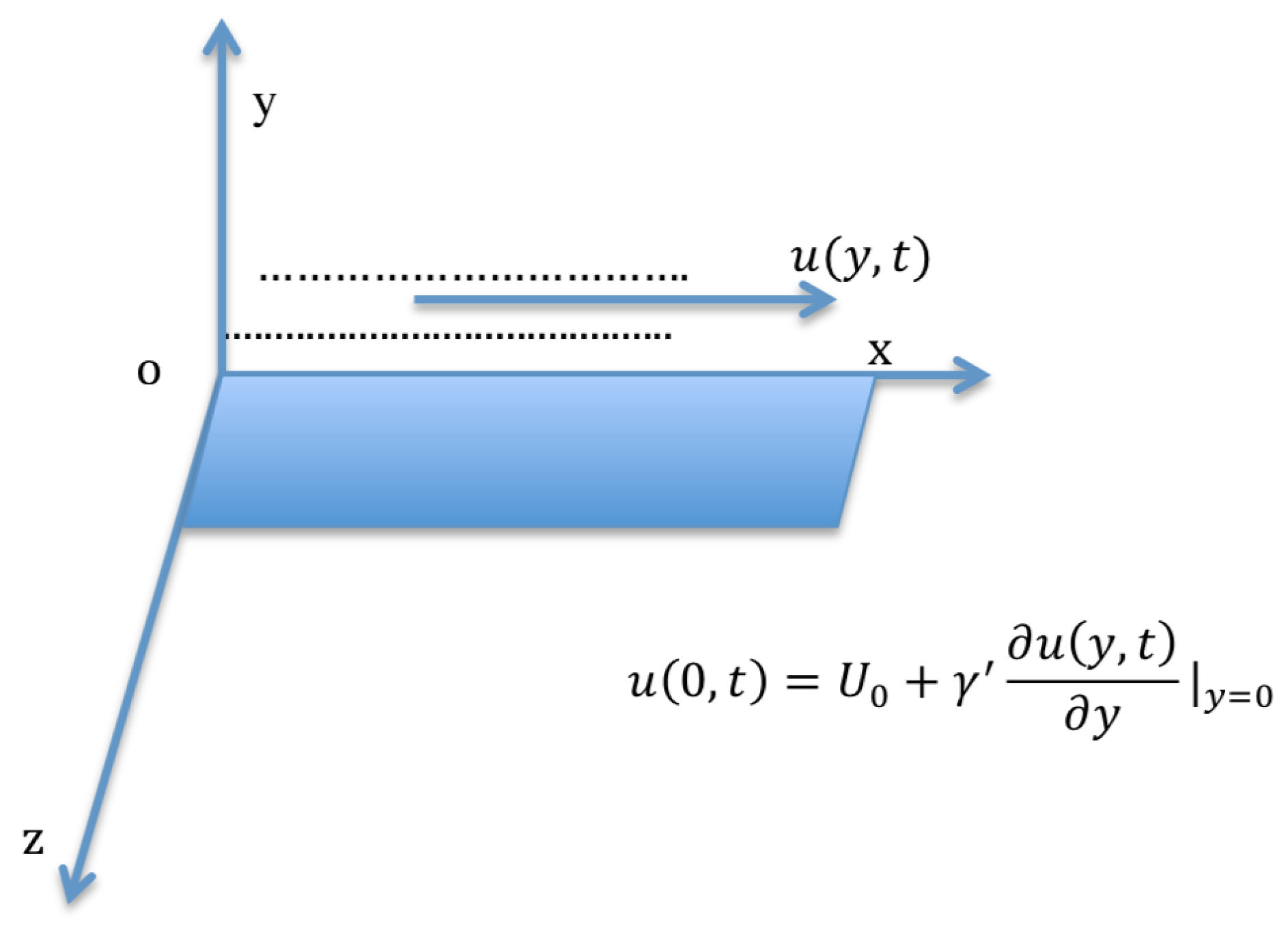
2. Mathematical Construction of the Problem

Let us consider an electrically conducting elasto-viscous fluid flowing past an infinite vertical plate (Figure 1). The plate is adjacent to the x-axis such that fluid is moving in this direction and y-axis is considered to be in the direction normal to flow. The initial temperature of plate, at rest, is taken to be $T_{\infty }$. The plate is given the motion $U_0$ in its own plane at $t=0^{+}$, causing the fluid to flow with slip. Simultaneously, the temperature of the plate is raised to be $T_W$. We shall be studying the unsteady motion of free-convected flow with slip and variable temperature. The magnetic field of uniform strength $B_0$ is applied in the normal direction of plate. We assume that the magnetic field is negligible in comparison to transverse magnetic field and Reynolds number is very small. The viscous dissipation and Soret & Duoffer effects due to lower level of concentration are assumed to be negligible. In regards to our model set-up, given conditions, above assumptions and Boussinesq approximation, elasto-viscous flow governing equations are given as [45]

$$\begin{array}{cc}\hfill \frac{\partial u(y,t)}{\partial t}& =\nu \frac{{\partial }^{2}u(y,t)}{\partial y^2}+g\beta (T(y,t)-T_{\infty })+g{\beta }^{*}(C(y,t)-C_{\infty })\hfill \\ & +\frac{K^{{}^{\prime }}}{\rho }\frac{{\partial }^{3}u(y,t)}{\partial y^2\partial t}-\frac{\sigma {B_0}^{2}u(y,t)}{\rho },y,t>0,\hfill \end{array}$$

(1)

$$\frac{\partial T(y,t)}{\partial t}=\frac{\kappa }{\rho C_p}\frac{{\partial }^{2}T(y,t)}{\partial y^2}-\frac{1}{\rho C_p}\frac{\partial q_r}{\partial y},y,t>0,$$

(2)

$$\frac{\partial C(y,t)}{\partial t}=D\frac{{\partial }^{2}C(y,t)}{\partial y^2},y,t>0,$$

(3)

with initial and boundary conditions as

$$u(y,0)=0,T(y,0)=T_{\infty },C(y,0)=C_{\infty },\mathrm{for}\mathrm{all}y\ge 0,$$

(4)

$$u(0,t)=U_0+{\gamma }^{{}^{\prime }}\frac{\partial u(y,t)}{\partial y}{|}_{y=0},U_0>0,$$

(5)

$$T(0,t)=T_{\infty }+T_W[1+af\left(t\right)],t>0,$$

(6)

$$C(0,t)=C_{\infty }+(C_W-C_{\infty })\frac{U_0^{2}t}{\nu },t>0,$$

(7)

$$u(y,t)\to 0,T(y,t)\to T_{\infty },C(y,t)\to C_{\infty },\mathrm{for}y\to \infty .$$

(8)

where $u(y,t)$, $T(y,t)$, $\rho$, $\nu$, $\sigma$, $\kappa$, $C_p$, $q_r$, $\beta$, ${\beta }^{*}$, $K^{{}^{\prime }}$, g, D represent velocity of the fluid, its temperature, density of fluid, kinematic viscosity, electrical conductivity, thermal conductivity, specific heat at constant pressure, radiation heat flux, thermal expansion coefficient, mass expansion coefficient, elasto-viscous parameter, gravitational acceleration and mass diffusion coefficient, respectively. Also, ${\gamma }^{{}^{\prime }}$ and a are constants. The slip between fluid and plate has been incorporated through ${\gamma }^{{}^{\prime }}$ in Equation (5).

Following non-dimensional variables have been employed for simplification of our system

$$\begin{array}{c}{u}^{*}=\frac{u}{U_0},y^{*}=\frac{y{U}_0}{\nu },t^{*}=\frac{t{U_0}^2}{\nu },T^{*}=\frac{T-T_{\infty }}{T_W},C^{*}=\frac{C-C_{\infty }}{C_W-C_{\infty }},\hfill \\ M=\frac{\sigma B_0^2{\nu }^2}{\mu U_0^2},G_r=\frac{g\beta T_W\nu }{U_0^3},K=\frac{K^{{}^{\prime }}{U}_0^2}{\mu \nu },G_m=\frac{g{\beta }^{*}\nu (C_W-C_{\infty })}{U_0^3},\hfill \\ P_r=\frac{\mu C_p}{\kappa },F=\frac{4I^{*}{\nu }^2}{\kappa U_0^2},S_c=\frac{\nu }{D},\hfill \end{array}$$

(9)

where M, $G_r$, $G_m$, F, $P_r$, $S_c$ and K denote Hartmann number, thermal Grashof number, mass Grashof number, thermal radiation parameter, Prandtl number, Schmidth number and elasto-viscous parameter, respectively.

Using non-dimensional entities (9), our system takes the form (dropping *)

$$\frac{\partial u(y,t)}{\partial t}=\frac{{\partial }^{2}u(y,t)}{\partial y^2}+G_{r}T(y,t)+G_{m}C(y,t)+K\frac{{\partial }^{3}u(y,t)}{\partial y^2\partial t}-Mu(y,t),$$

(10)

$$\frac{\partial T(y,t)}{\partial t}=\frac{1}{P_r}\frac{{\partial }^{2}T(y,t)}{\partial y^2}-\frac{F}{P_r}T(y,t),$$

(11)

$$\frac{\partial C(y,t)}{\partial t}=\frac{1}{S_c}\frac{{\partial }^{2}C(y,t)}{\partial y^2},$$

(12)

$$u(y,0)=0,T(y,0)=0,C(y,0)=0,\mathrm{for}\mathrm{all}y\ge 0,$$

(13)

$$u(0,t)=1+\gamma \frac{\partial u(y,t)}{\partial y}{|}_{y=0},t>0,$$

(14)

$$T(0,t)=1+af\left(t\right),t>0,$$

(15)

$$C(0,t)=t,t>0,$$

(16)

$$u(y,t)\to 0,T(y,t)\to 0,C(y,t)\to 0,\mathrm{as}y\to \infty .$$

(17)

3. Mathematical Solutions

The exact expression of concentration field $C(y,t)$ has been determined by taking Laplace transform of Equation (12) with the help of conditions (16) and (17). We obtain

$$\overline{C}(y,q)=\frac{e^{-\sqrt{S_{c}q}y}}{q^2}.$$

(18)

Laplace inverse transform of Equation (18) gives

$$C(y,t)={\int }_0^{t}erfc\left(\frac{\sqrt{S_c}y}{2\sqrt{s}}\right)ds,$$

or

$$C(y,t)=terfc\left(\frac{\sqrt{S_c}y}{2\sqrt{t}}\right)-\frac{\sqrt{S_c}y}{2}{\int }_0^t\frac{e^{-\frac{S_c{y}^2}{4s}}}{\sqrt{\pi s}}ds.$$

(19)

To find the exact expression for temperature of fluid, $T(y,t)$, we take Laplace transform of Equation (11) and using conditions (15) and (17), we get

$$\overline{T}(y,q)=\frac{e^{-\sqrt{P_r(q+\alpha )}y}}{q}+aF\left(q\right)e^{-\sqrt{P_r(q+\alpha )}y},$$

(20)

where $\alpha =\frac{F}{P_r}$.

Laplace inverse transform of Equation (20) gives

$$\begin{array}{cc}\hfill T(y,t)& =\frac{1}{2}\left[e^{\sqrt{\alpha P_r}y}erfc\left(\frac{\sqrt{P_r}y}{2\sqrt{t}}+\sqrt{\alpha t}\right)+e^{-\sqrt{\alpha P_r}y}erfc\left(\frac{\sqrt{P_r}y}{2\sqrt{t}}-\sqrt{\alpha t}\right)\right]\hfill \\ \hfill & +\frac{a\sqrt{P_r}}{2}{\int }_0^{t}f(t-s)\frac{y}{\sqrt{\pi {\left(s\right)}^3}}{e}^{-\alpha s-\frac{P_r{y}^2}{4s}}ds,\hfill \end{array}$$

(21)

satisfying both initial and boundary conditions.

Now, to obtain the closed form solution of velocity field of elasto-viscous fluid, we take Laplace transform of Equation (10), i.e.,

$$q\overline{u}(y,q)=\frac{{\partial }^2\overline{u}(y,q)}{\partial y^2}+G_r\overline{T}(y,q)+G_m\overline{C}(y,q)+Kq\frac{{\partial }^2\overline{u}(y,q)}{\partial y^2}-M\overline{u}(y,q).$$

(22)

Solving Equation (22) using Laplace transform of Equations (13), (14) and (17), we obtain

$$\begin{array}{cc}\hfill \overline{u}(y,q)& =\frac{e^{-\sqrt{\frac{q+M}{1+Kq}}y}}{q(1+\gamma \sqrt{\frac{}{}}q+M1+Kq)}+\frac{G_r{e}^{-\sqrt{\frac{q+M}{1+Kq}}y}}{P_{r}Kq(1+\gamma \sqrt{\frac{}{}}q+M1+Kq)[{(q-d)}^2-{\left(\sqrt{c}\right)}^2]}\hfill \\ & +\frac{a{G}_{r}F\left(q\right)e^{-\sqrt{\frac{q+M}{1+Kq}}y}}{P_{r}K(1+\gamma \sqrt{\frac{}{}}q+M1+Kq)[{(q-d)}^2-{\left(\sqrt{c}\right)}^2]}+\frac{G_m{e}^{-\sqrt{\frac{q+M}{1+Kq}}y}}{S_{c}K{q}^2(1+\gamma \sqrt{\frac{}{}}q+M1+Kq)[{(q-h)}^2-{\left(\sqrt{l}\right)}^2]}\hfill \\ & +\frac{\gamma G_r\sqrt{F+P_{r}q}{e}^{-\sqrt{\frac{q+M}{1+Kq}}y}}{P_{r}K(1+\gamma \sqrt{\frac{}{}}q+M1+Kq)q[{(q-d)}^2-{\left(\sqrt{c}\right)}^2]}+\frac{\gamma a{G}_{r}F\left(q\right)\sqrt{F+P_{r}q}{e}^{-\sqrt{\frac{q+M}{1+Kq}}y}}{P_{r}K(1+\gamma \sqrt{\frac{}{}}q+M1+Kq)[{(q-d)}^2-{\left(\sqrt{c}\right)}^2]}\hfill \\ & +\frac{\gamma G_m\sqrt{S_{c}q}{e}^{-\sqrt{\frac{q+M}{1+Kq}}y}}{S_{c}K{q}^2(1+\gamma \sqrt{\frac{}{}}q+M1+Kq)[{(q-h)}^2-{\left(\sqrt{l}\right)}^2]}-\frac{G_r{e}^{-\sqrt{P_r(q+\alpha )}y}}{P_{r}Kq[{(q-d)}^2-{\left(\sqrt{c}\right)}^2]}\hfill \\ & -\frac{a{G}_{r}F\left(q\right)e^{-\sqrt{P_r(q+\alpha )}y}}{P_{r}K[{(q-d)}^2-{\left(\sqrt{c}\right)}^2]}-\frac{G_m{e}^{-\sqrt{S_{c}q}y}}{S_{c}K{q}^2[{(q-h)}^2-{\left(\sqrt{l}\right)}^2]}.\hfill \end{array}$$

(23)

Equation (23) can be written in a more simplified form o determine the Laplace inverse such as

$$\begin{array}{cc}\hfill \overline{u}(y,q)=& G_1(y,q)\frac{1}{q}+\frac{G_r}{P_{r}K}{G}_1(y,q)\frac{1}{q[{(q-d)}^2-{\left(\sqrt{c}\right)}^2]}+\frac{a{G}_r}{P_{r}K}{G}_1(y,q)F\left(q\right)\frac{1}{[{(q-d)}^2-{\left(\sqrt{c}\right)}^2]}\hfill \\ & +\frac{G_m}{S_{c}K}{G}_1(y,q)\frac{1}{q^2[{(q-h)}^2-{\left(\sqrt{l}\right)}^2]}+\frac{\gamma G_r}{P_{r}K}{G}_1(y,q)\frac{\sqrt{F+P_{r}q}}{q[{(q-d)}^2-{\left(\sqrt{c}\right)}^2]}\hfill \\ & +\frac{\gamma a{G}_r}{P_{r}K}{G}_1(y,q)F\left(q\right)\frac{\sqrt{F+P_{r}q}}{[{(q-d)}^2-{\left(\sqrt{c}\right)}^2]}+\frac{\gamma G_m}{\sqrt{S_c}K}{G}_1(y,q)\frac{1}{\sqrt{q}\left(q[{(q-h)}^2-{\left(\sqrt{l}\right)}^2]\right)}\hfill \\ & -\frac{G_r}{P_{r}K}\frac{e^{-\sqrt{P_r(q+\alpha )}y}}{q[{(q-d)}^2-{\left(\sqrt{c}\right)}^2]}-\frac{a{G}_r}{P_{r}K}F\left(q\right)\frac{e^{-\sqrt{P_r(q+\alpha )}y}}{[{(q-d)}^2-{\left(\sqrt{c}\right)}^2]}-\frac{G_m}{S_{c}K}\frac{e^{-\sqrt{S_{c}q}y}}{q^2[{(q-h)}^2-{\left(\sqrt{l}\right)}^2]},\hfill \end{array}$$

(24)

where

$$\begin{array}{cc}\hfill d=& \frac{1-P_r-FK}{2P_{r}K},c={\left(\frac{1-P_r-FK}{2P_{r}K}\right)}^2-\frac{F-M}{P_{r}K},G_1(y,q)=\frac{e^{-\sqrt{\frac{q+M}{1+Kq}}y}}{\gamma \left(\sqrt{\frac{q+M}{1+Kq}}+\frac{1}{\gamma }\right)},\\ \hfill & h=\frac{1-S_c}{2S_{c}K},l={\left(\frac{1-S_c}{2S_{c}K}\right)}^2+\frac{M}{S_{c}K}.\end{array}$$

Taking Laplace inverse transform of Equation (24) and using (A1)–(A12), we obtain the exact expression for velocity field

$$\begin{array}{c}u(y,t)=\left(1+\frac{G_r}{(d^2-c)P_{r}K}+\frac{2G_{m}h}{S_{c}K{(h^2-l)}^2}\right){\int }_0^t{g}_1(y,s)ds+\frac{G_r}{2P_{r}K(c+d\sqrt{c})}{\int }_0^t{g}_1(y,s)e^{(d+\sqrt{c})(t-s)}ds\hfill \\ +\frac{G_r}{2P_{r}K(c-d\sqrt{c})}{\int }_0^t{g}_1(y,s)e^{(d-\sqrt{c})(t-s)}ds+\frac{a{G}_r}{2P_{r}K\sqrt{c}}{\int }_0^t{g}_1(y,s)H_1(t-s)ds\hfill \\ -\frac{a{G}_r}{2P_{r}K\sqrt{c}}{\int }_0^t{g}_1(y,s)H_2(t-s)ds+\frac{G_m}{S_{c}K(h^2-l)}{\int }_0^t{g}_1(y,s)(t-s)ds\hfill \\ +\frac{G_m}{S_{c}K\left[2\sqrt{l}{(h+\sqrt{l})}^2\right]}{\int }_0^t{g}_1(y,s)e^{(h+\sqrt{l})(t-s)}ds-\frac{G_m}{S_{c}K\left[2\sqrt{l}{(h-\sqrt{l})}^2\right]}{\int }_0^t{g}_1(y,s)e^{(h-\sqrt{l})(t-s)}ds\hfill \\ +\frac{\gamma G_r}{K\sqrt{P_r}(d^2-c)}{\int }_0^t{g}_1(y,s)\left\{\frac{e^{-\alpha (t-s)}}{\sqrt{\pi (t-s)}}+\sqrt{\alpha }erf\left(\sqrt{\alpha (t-s)}\right)\right\}ds\hfill \\ +\frac{\gamma G_r}{2K\sqrt{P_r}(c+d\sqrt{c})}{\int }_0^t{g}_1(y,s)\left\{\frac{e^{-\alpha (t-s)}}{\sqrt{\pi (t-s)}}+\sqrt{\alpha +d+\sqrt{c}}{e}^{(d+\sqrt{c})(t-s)}erf\left(\sqrt{(\alpha +d+\sqrt{c})(t-s)}\right)\right\}ds\hfill \\ +\frac{\gamma G_r}{2K\sqrt{P_r}(c-d\sqrt{c})}{\int }_0^t{g}_1(y,s)\left\{\frac{e^{-\alpha (t-s)}}{\sqrt{\pi (t-s)}}+\sqrt{\alpha +d-\sqrt{c}}{e}^{(d-\sqrt{c})(t-s)}erf\left(\sqrt{(\alpha +d-\sqrt{c})(t-s)}\right)\right\}ds\hfill \\ +\frac{\gamma a{G}_r}{2K{P}_r\sqrt{c}}{\int }_0^t{g}_1(y,s)R_1(t-s)ds-\frac{\gamma a{G}_r}{2K{P}_r\sqrt{c}}{\int }_0^t{g}_1(y,s)R_2(t-s)ds+\frac{2\gamma G_m}{K\sqrt{\pi S_c}(h^2-l)}{\int }_0^t{g}_1(y,s)\sqrt{t-s}ds\hfill \\ +\frac{\gamma G_m}{2\sqrt{l{S}_c}K{(h+\sqrt{l})}^{\frac{3}{2}}}{\int }_0^t{g}_1(y,s)e^{(h+\sqrt{l})(t-s)}erf\left(\sqrt{(h+\sqrt{l})(t-s)}\right)ds\hfill \\ -\frac{\gamma G_m}{2\sqrt{l{S}_c}K{(h-\sqrt{l})}^{\frac{3}{2}}}{\int }_0^t{g}_1(y,s)e^{(h-\sqrt{l})(t-s)}erf\left(\sqrt{(h-\sqrt{l})(t-s)}\right)ds\hfill \\ -\frac{G_r}{2P_{r}K(d^2-c)}\left[e^{y\sqrt{\alpha P_r}}erfc\left(\frac{\sqrt{P_r}y}{2\sqrt{t}}+\sqrt{\alpha t}\right)+e^{-y\sqrt{\alpha P_r}}erfc\left(\frac{\sqrt{P_r}y}{2\sqrt{t}}-\sqrt{\alpha t}\right)\right]\hfill \\ +\frac{G_{m}y}{2\sqrt{S_c}K(h^2-l)}{\int }_0^t\frac{e^{\frac{-P_r{y}^2}{4s}}}{\sqrt{\pi s}}ds-\frac{G_r{e}^{(d+\sqrt{c})t}}{4P_{r}K(c+d\sqrt{c})}[e^{y\sqrt{(\alpha +d+\sqrt{c})P_r}}erfc\left(\frac{\sqrt{P_r}y}{2\sqrt{t}}+\sqrt{(\alpha +d+\sqrt{c}t}\right)\hfill \\ +e^{-y\sqrt{(\alpha +d+\sqrt{c})P_r}}erfc\left(\frac{\sqrt{P_r}y}{2\sqrt{t}}-\sqrt{(\alpha +d+\sqrt{c}t}\right)]\hfill \\ -\frac{G_r{e}^{(d-\sqrt{c})t}}{4P_{r}K(c-d\sqrt{c})}[e^{y\sqrt{(\alpha +d-\sqrt{c})P_r}}erfc\left(\frac{\sqrt{P_r}y}{2\sqrt{t}}+\sqrt{(\alpha +d-\sqrt{c}t}\right)\hfill \\ +e^{-y\sqrt{(\alpha +d-\sqrt{c})P_r}}erfc\left(\frac{\sqrt{P_r}y}{2\sqrt{t}}-\sqrt{(\alpha +d-\sqrt{c}t}\right)]-\frac{a{G}_{r}y}{4K\sqrt{c{P}_r}}{\int }_0^t\frac{e^{\frac{-P_r{y}^2}{4s}-\alpha s}}{\sqrt{\pi s^3}}{H}_1(t-s)ds\hfill \\ +\frac{a{G}_{r}y}{4K\sqrt{c{P}_r}}{\int }_0^t\frac{e^{\frac{-P_r{y}^2}{4s}-\alpha s}}{\sqrt{\pi s^3}}{H}_2(t-s)ds-\frac{G_m(2h+(h^2-l)t)}{S_{c}K{(h^2-l)}^2}erfc\left(\frac{\sqrt{S_c}y}{2\sqrt{t}}\right)\hfill \\ -\frac{G_m{e}^{(h+\sqrt{l})t}}{4S_{c}K\sqrt{l}{(h+\sqrt{l})}^2}[e^{y\sqrt{(h+\sqrt{l})S_c}}erfc\left(\frac{\sqrt{S_c}y}{2\sqrt{t}}+\sqrt{(h+\sqrt{l})t}\right)\hfill \\ +e^{-y\sqrt{(h+\sqrt{l})S_c}}erfc\left(\frac{\sqrt{S_c}y}{2\sqrt{t}}-\sqrt{(h+\sqrt{l})t}\right)]\hfill \\ +\frac{G_m{e}^{(h-\sqrt{l})t}}{4S_{c}K\sqrt{l}{(h-\sqrt{l})}^2}[e^{y\sqrt{(h-\sqrt{l})S_c}}erfc\left(\frac{\sqrt{S_c}y}{2\sqrt{t}}+\sqrt{(h-\sqrt{l})t}\right)\hfill \\ +e^{-y\sqrt{(h-\sqrt{l})S_c}}erfc\left(\frac{\sqrt{S_c}y}{2\sqrt{t}}-\sqrt{(h-\sqrt{l})t}\right)],\hfill \end{array}$$

(25)

satisfying initial and boundary conditions, where

$$g_1(y,t)=L^{-1}\left\{G_1(y,q)\right\}=L^{-1}\left\{\left(F_{1}oW\right)\left(q\right)\right\}=L^{-1}\left\{F_1\left(W\left(q\right)\right)\right\}={\int }_0^{\infty }{f}_1(y,z)p(z,t)dz,$$

$$f_1(y,t)=L^{-1}\left\{F_1(y,q)\right\}=L^{-1}\left\{\frac{e^{-\sqrt{q}y}}{\gamma \left(\sqrt{q}+\frac{1}{\gamma }\right)}\right\}=\frac{1}{\gamma }\left\{\frac{e^{-\frac{y^2}{4t}}}{\sqrt{\pi t}}-\frac{1}{\gamma }{e}^{\frac{y}{\gamma }+\frac{t}{{\gamma }^2}}erfc\left(\frac{y}{2\sqrt{t}}+\frac{\sqrt{t}}{\gamma }\right)\right\},$$

$$W\left(q\right)=\frac{q+M}{1+Kq},p(z,t)=L^{-1}\left\{e^{-zW\left(q\right)}\right\}=e^{\frac{z}{K}}\left[\sqrt{\frac{\mathcal{N}}{t}}{I}_1\left(2\sqrt{\mathcal{N}}t\right)e^{\frac{t}{K}}+\delta \left(t\right)\right],$$

($I_1$ is modified Bessel function of first kind of order 1, $\delta \left(t\right)$ represents the delta function and $\mathcal{N}=\frac{z(MK+1)}{K^2}$)

$$H_1\left(t\right)=L^{-1}\left\{\frac{F\left(q\right)}{q-(d+\sqrt{c})}\right\}={\int }_0^{t}f\left(s\right)e^{(d+\sqrt{c})(t-s)}ds,$$

$$H_2\left(t\right)=L^{-1}\left\{\frac{F\left(q\right)}{q-(d-\sqrt{c})}\right\}={\int }_0^{t}f\left(s\right)e^{(d-\sqrt{c})(t-s)}ds,$$

$$\begin{array}{cc}\hfill R_1\left(t\right)& =L^{-1}\left\{F\left(q\right)\frac{\sqrt{F+P_{r}q}}{q-(d+\sqrt{c})}\right\}\hfill \\ & ={\int }_0^{t}f\left(s\right)\left[\frac{e^{-\alpha (t-s)}}{\sqrt{\pi (t-s)}}+\sqrt{\alpha +d+\sqrt{c}}{e}^{(d+\sqrt{c})(t-s)}erf(\sqrt{(\alpha +d+\sqrt{c})(t-s)}\right]ds,\hfill \end{array}$$

$$\begin{array}{cc}\hfill R_2\left(t\right)& =L^{-1}\left\{F\left(q\right)\frac{\sqrt{F+P_{r}q}}{q-(d-\sqrt{c})}\right\}\hfill \\ & ={\int }_0^{t}f\left(s\right)\left[\frac{e^{-\alpha (t-s)}}{\sqrt{\pi (t-s)}}+\sqrt{\alpha +d-\sqrt{c}}{e}^{(d-\sqrt{c})(t-s)}erf(\sqrt{(\alpha +d-\sqrt{c})(t-s)}\right]ds.\hfill \end{array}$$

4. Limiting Cases

To check the veracity of our exact solutions, as well as to study the influence of varying parametric values, limiting solutions have been calculated. The expression of velocity corresponding to Newtonian fluid flow, both in the presence and absence of magnetic fields, shall be determined. The impact of constant temperature provision on the boundary of plate and constant velocity on boundary will also be studied through approximation of fluid parameters.

4.1. Newtonian Fluid

The elasto-viscous fluid model reduces to Newtonian fluid system when K is considered to be very small (Equation (10)). Following this, Equation (23) becomes

$$\begin{array}{cc}\hfill \overline{u}(y,q)& =\frac{e^{-\sqrt{q+M}y}}{q(1+\sqrt{q+M})}+\frac{G_r\sqrt{F+P_{r}q}{e}^{-\sqrt{q+M}y}}{(P_r-1)q(q-m)(1+\sqrt{q+M})}\hfill \\ & +\frac{a{G}_r\sqrt{F+P_{r}q}{e}^{-\sqrt{q+M}y}}{(P_r-1)(q-m)(1+\sqrt{q+M})}+\frac{G_m\sqrt{S_{c}q}{e}^{-\sqrt{q+M}y}}{(S_c-1)q^2(q-m)(1+\sqrt{q+M})}\hfill \\ & +\frac{G_r{e}^{-\sqrt{q+M}y}}{(P_r-1)q(q-m)(1+\sqrt{q+M})}+\frac{a{G}_r{e}^{-\sqrt{q+M}y}}{(P_r-1)(q-m)(1+\sqrt{q+M})}\hfill \\ & +\frac{G_m{e}^{-\sqrt{q+M}y}}{(S_c-1)q^2(q-h)(1+\sqrt{q+M})}-\frac{G_r{e}^{-\sqrt{F+P_{r}q}y}}{(P_r-1)q(q-m)}\hfill \\ & -\frac{a{G}_r{e}^{-\sqrt{F+P_{r}q}y}}{(P_r-1)(q-m)}-\frac{G_m{e}^{-\sqrt{S_{c}q}y}}{(S_c-1)q^2(q-n)},\hfill \end{array}$$

(26)

where

$$\begin{array}{c}\hfill m=\frac{M-F}{P_r-1},n=\frac{M}{S_c-1}.\end{array}$$

To find Inverse Laplace transform, we write Equation (26) in the following way

$$\begin{array}{cc}\hfill \overline{u}(y,q)& =\frac{e^{-\sqrt{q+M}y}}{(1+\sqrt{q+M})}\frac{1}{q}+\frac{G_r}{(P_r-1)}\frac{e^{-\sqrt{q+M}y}}{(1+\sqrt{q+M})}\frac{\sqrt{F+P_{r}q}}{q(q-m)}\hfill \\ & +\frac{a{G}_r}{(P_r-1)}\frac{e^{-\sqrt{q+M}y}}{(1+\sqrt{q+M})}\frac{\sqrt{F+P_{r}q}}{q-m}+\frac{G_m\sqrt{S_c}}{S_c-1}\frac{e^{-\sqrt{q+M}y}}{(1+\sqrt{q+M})}\frac{\sqrt{q}}{q^2(q-m)}\hfill \\ & +\frac{G_r}{P_r-1}\frac{e^{-\sqrt{q+M}y}}{(1+\sqrt{q+M})}\frac{1}{q(q-m)}+\frac{a{G}_r}{(P_r-1)}\frac{e^{-\sqrt{q+M}y}}{(1+\sqrt{q+M})}\frac{1}{q-m}\hfill \\ & +\frac{G_m}{(S_c-1)}\frac{e^{-\sqrt{q+M}y}}{(1+\sqrt{q+M})}\frac{1}{q^2(q-n)}-\frac{G_r}{(P_r-1)}\frac{e^{-\sqrt{F+P_{r}q}}}{q(q-m)}\hfill \\ & -\frac{a{G}_r}{(P_r-1)}\frac{e^{-\sqrt{F+P_{r}q}}}{q-m}-\frac{G_m}{S_c-1}\frac{e^{-\sqrt{S_{c}q}y}}{q^2(q-n)}.\hfill \end{array}$$

(27)

Taking the Inverse Laplace transform of Equation (27) and using (A3), (A5) and (A6), we get

$$\begin{array}{c}u(y,t)=\left(1-\frac{G_r}{m(P_r-1)}-\frac{G_m}{n^2(S_c-l)}\right){\int }_0^t{g}_2(y,s)ds\hfill \\ -\frac{G_r\sqrt{P_r}}{m(P_r-1)}{\int }_0^t{g}_2(y,s)\left\{\frac{e^{-\alpha (t-s)}}{\sqrt{\pi (t-s)}}+\sqrt{\alpha }erf\left(\sqrt{\alpha (t-s)}\right)\right\}ds\hfill \\ +\frac{G_r\sqrt{P_r}}{m(P_r-1)}{\int }_0^t{g}_2(y,s)\left\{\frac{e^{-\alpha (t-s)}}{\sqrt{\pi (t-s)}}+\sqrt{\alpha +m}{e}^{m(t-s)}erf\left(\sqrt{(\alpha +m)(t-s)}\right)\right\}ds\hfill \\ +\frac{a{G}_r\sqrt{P_r}}{(P_r-1)}{\int }_0^t{g}_2(y,s)\left\{\frac{e^{-\alpha (t-s)}}{\sqrt{\pi (t-s)}}+\sqrt{\alpha +m}{e}^{m(t-s)}erf\left(\sqrt{(\alpha +m)(t-s)}\right)\right\}ds\hfill \\ +\frac{G_m\sqrt{S_c}}{S_c-1}{\int }_0^t{g}_2(y,s)\psi (t-s)ds+\frac{G_r}{m(P_r-1)}{\int }_0^t{g}_2(y,s)e^{m(t-s)}ds+\frac{a{G}_r}{P_r-1}{\int }_0^t{g}_2(y,s)e^{m(t-s)}ds\hfill \\ -\frac{G_m}{n(S_c-1)}{\int }_0^t{g}_2(y,s)(t-s)ds+\frac{G_m}{n^2(S_c-1)}{\int }_0^t{g}_2(y,s)e^{n(t-s)}ds+\frac{G_r}{m(P_r-1)}erfc\left(\frac{\sqrt{P_r}y}{2\sqrt{t}}\right)e^{-\alpha t}\hfill \\ -\frac{G_r{e}^{mt}(1+a)}{2m(P_r-1)}\left[e^{y\sqrt{(\alpha +m)P_r}}erfc\left(\frac{\sqrt{P_r}y}{2\sqrt{t}}+\sqrt{(\alpha +m)t}\right)+e^{-y\sqrt{(\alpha +m)P_r}}erfc\left(\frac{\sqrt{P_r}y}{2\sqrt{t}}-\sqrt{(\alpha +m)t}\right)\right]\hfill \\ +\frac{G_m}{n^2(S_c-1)}erfc\left(\frac{\sqrt{S_{c}y}}{2\sqrt{t}}\right)+\frac{G_m}{n(S_c-1)}{\int }_0^{t}erfc\left(\frac{\sqrt{S_{c}y}}{2\sqrt{s}}\right)ds\hfill \\ -\frac{G_m{e}^{nt}}{2n^2(S_c-1)}\left[e^{y\sqrt{n{S}_c}}erfc\left(\frac{\sqrt{S_c}y}{2\sqrt{t}}+\sqrt{nt}\right)+e^{-y\sqrt{n{S}_c}}erfc\left(\frac{\sqrt{S_c}y}{2\sqrt{t}}-\sqrt{nt}\right)\right],\hfill \end{array}$$

(28)

where

$$\begin{array}{c}\hfill g_2(y,t)=L^{-1}\left\{G_2(y,q)\right\}=L^{-1}\left\{\frac{e^{-\sqrt{q+M}}}{\sqrt{q+M}+1}\right\}=\frac{e^{-\frac{y^2}{4t}-Mt}}{\sqrt{\pi t}}-e^{y+t-Mt}erfc\left(\frac{y}{2\sqrt{t}}+\sqrt{t}\right).\end{array}$$

4.2. Absence of Magnetic Field ($M\to 0$)

The expression of velocity field for the case of Newtonian fluid ($K\to 0$) and no magnetic field ($M\to 0$), takes the form

$$\begin{array}{cc}\hfill u(y,t)& =\left(1+\frac{G_r}{F}\right){\int }_0^t{g}_3(y,s)ds+\frac{G_r\sqrt{P_r}}{F}{\int }_0^t{g}_3(y,s)\left\{\frac{e^{-\alpha (t-s)}}{\sqrt{\pi (t-s)}}+\sqrt{\alpha }erf\left(\sqrt{\alpha (t-s)}\right)\right\}ds\hfill \\ & -\left(\frac{G_r\sqrt{P_r}}{F}+\frac{a{G}_r\sqrt{P_r}}{P_r-1}\right){\int }_0^t{g}_3(y,s)\left\{\frac{e^{-\alpha (t-s)}}{\sqrt{\pi (t-s)}}+\sqrt{\zeta }{e}^{\frac{-F}{P_r-1}(t-s)}erf\left(\sqrt{\zeta (t-s)}\right)\right\}ds\hfill \\ & +\frac{G_m\sqrt{S_c}}{S_c-1}{\int }_0^t{g}_3(y,s){\psi }_2(t-s)ds-\left(\frac{G_r}{F}-\frac{a{G}_r}{P_r-1}\right){\int }_0^t{g}_3(y,s)e^{\frac{-F}{P_r-1}(t-s)}ds\hfill \\ & +\frac{G_m}{S_c-1}{\int }_0^t{g}_3(y,s){(t-s)}^{2}ds-\frac{G_r}{F}erfc\left(\frac{y\sqrt{P_r}}{2\sqrt{t}}\right)e^{-\alpha t}-\frac{G_m}{S_c-1}{\int }_0^{t}erfc\left(\frac{\sqrt{S_c}y}{2\sqrt{s}}\right)(t-s)ds\hfill \\ & +\frac{G_r(1+a)e^{-\frac{Ft}{P_r-1}}}{2F}\left[e^{y\sqrt{\zeta P_r}-\frac{F}{P_r-1}t}erfc\left(\frac{\sqrt{P_r}y}{2\sqrt{t}}+\sqrt{\zeta t}\right)+e^{y\sqrt{\zeta P_r}-\frac{F}{P_r-1}t}erfc\left(\frac{\sqrt{P_r}y}{2\sqrt{t}}-\sqrt{\zeta t}\right)\right],\hfill \end{array}$$

(29)

where

$$\zeta =\frac{F}{P_r(P_r-1)},g_3(y,t)=L^{-1}\left\{G_3(y,q)\right\}=L^{-1}\left\{\frac{e^{-\sqrt{q}}}{\sqrt{q}+1}\right\}=\frac{e^{-\frac{y^2}{4t}}}{\sqrt{\pi t}}-e^{y+t}erfc\left(\frac{y}{2\sqrt{t}}+\sqrt{t}\right),$$

$${\psi }_2\left(t\right)={\int }_0^{t}2\sqrt{\frac{s}{\sqrt{\pi }}}{e}^{-\frac{F}{P_r-1}(t-s)}ds.$$

4.3. Constant Temperature on the Boundary

We have also retrieved the results for temperature and velocity for the case of Newtonian fluid ($K\to 0$) and constant temperature on the boundary ($a=0$) as following

$$T(y,t)=\frac{1}{2}\left[e^{\sqrt{\alpha P_r}y}erfc\left(\frac{\sqrt{P_r}y}{2\sqrt{t}}+\sqrt{\alpha t}\right)+e^{-\sqrt{\alpha P_r}y}erfc\left(\frac{\sqrt{P_r}y}{2\sqrt{t}}-\sqrt{\alpha t}\right)\right],$$

(30)

and

$$\begin{array}{c}u(y,t)=\left(1-\frac{G_r}{m(P_r-1)}-\frac{G_m}{n^2(S_c-1)}\right){\int }_0^t{g}_2(y,s)ds\hfill \\ -\frac{G_r\sqrt{P_r}}{m(P_r-1)}{\int }_0^t{g}_2(y,s)\left\{\frac{e^{-\alpha (t-s)}}{\sqrt{\pi (t-s)}}+\sqrt{\alpha }erf\left(\sqrt{\alpha (t-s)}\right)\right\}ds\hfill \\ +\frac{G_r\sqrt{P_r}}{m(P_r-1)}{\int }_0^t{g}_2(y,s)\left\{\frac{e^{-\alpha (t-s)}}{\sqrt{\pi (t-s)}}+\sqrt{m+\alpha }{e}^{m(t-s)}erf\left(\sqrt{(m+\alpha )(t-s)}\right)\right\}ds\hfill \\ +\frac{G_m\sqrt{S_c}}{S_c-1}{\int }_0^t{g}_2(y,s)\psi (t-s)ds+\frac{G_r}{m\left(P_r\right)}{\int }_0^t{g}_2(y,s)e^{m(t-s)}ds\hfill \\ -\frac{G_m}{n(S_c-1)}{\int }_0^t{g}_2(y,s)(t-s)ds+\frac{G_r}{m(P_r-1)}erfc\left(\frac{y\sqrt{P_r}}{2\sqrt{t}}\right)e^{-\alpha t}\hfill \\ +\frac{G_m}{n^2(S_c-1)}{\int }_0^t{g}_2(y,s)e^{n(t-s)}ds+\frac{G_r(1+a)}{2F}[e^{y\sqrt{\zeta P_r}-\frac{F}{P_r-1}t}erfc\left(\frac{\sqrt{P_r}y}{2\sqrt{t}}+\sqrt{\zeta t}\right)\hfill \\ +e^{y\sqrt{\zeta P_r}-\frac{F}{P_r-1}t}erfc\left(\frac{\sqrt{P_r}y}{2\sqrt{t}}-\sqrt{\zeta t}\right)]-\frac{G_r{e}^{mt}(1+a)}{2m(P_r-1)}[e^{y\sqrt{(\alpha +m)P_r}}erfc\left(\frac{\sqrt{P_r}y}{2\sqrt{t}}+\sqrt{(\alpha +m)t}\right)\hfill \\ +e^{-y\sqrt{(\alpha +m)P_r}}erfc\left(\frac{\sqrt{P_r}y}{2\sqrt{t}}-\sqrt{(\alpha +m)t}\right)]\hfill \\ +\frac{G_m}{n^2(S_c-1)}erfc\left(\frac{\sqrt{S_{c}y}}{2\sqrt{t}}\right)+\frac{G_m}{n(S_c-1)}{\int }_0^{t}erfc\left(\frac{\sqrt{S_{c}y}}{2\sqrt{s}}\right)ds\hfill \\ -\frac{G_m{e}^{nt}}{2n^2(S_c-1)}\left[e^{y\sqrt{n{S}_c}}erfc\left(\frac{\sqrt{S_c}y}{2\sqrt{t}}+\sqrt{nt}\right)+e^{-y\sqrt{n{S}_c}}erfc\left(\frac{\sqrt{S_c}y}{2\sqrt{t}}-\sqrt{nt}\right)\right],\hfill \end{array}$$

(31)

where

$$\begin{array}{cc}\hfill \psi \left(t\right)& =L^{-1}\left\{\frac{e^{-\sqrt{P_r}y\sqrt{q}}}{q-(d-\sqrt{c})}\right\}={\int }_0^t\frac{\sqrt{P_r}y{e}^{-\frac{P_r{y}^2}{4u}}}{2u\sqrt{\pi u}}{e}^{(d-\sqrt{c})(t-u)}du\hfill \\ & =\frac{\sqrt{P_r}{e}^{(d-\sqrt{c})t}}{2}\left[e^{y\sqrt{P_r(d-\sqrt{c})}}erfc\left(\frac{\sqrt{P_r}y}{2\sqrt{t}}+\sqrt{(d-\sqrt{c})t}\right)+e^{-y\sqrt{P_r(d-\sqrt{c})}}erfc\left(\frac{\sqrt{P_r}y}{2\sqrt{t}}-\sqrt{(d-\sqrt{c})t}\right)\right].\hfill \end{array}$$

4.4. Constant Velocity on Boundary

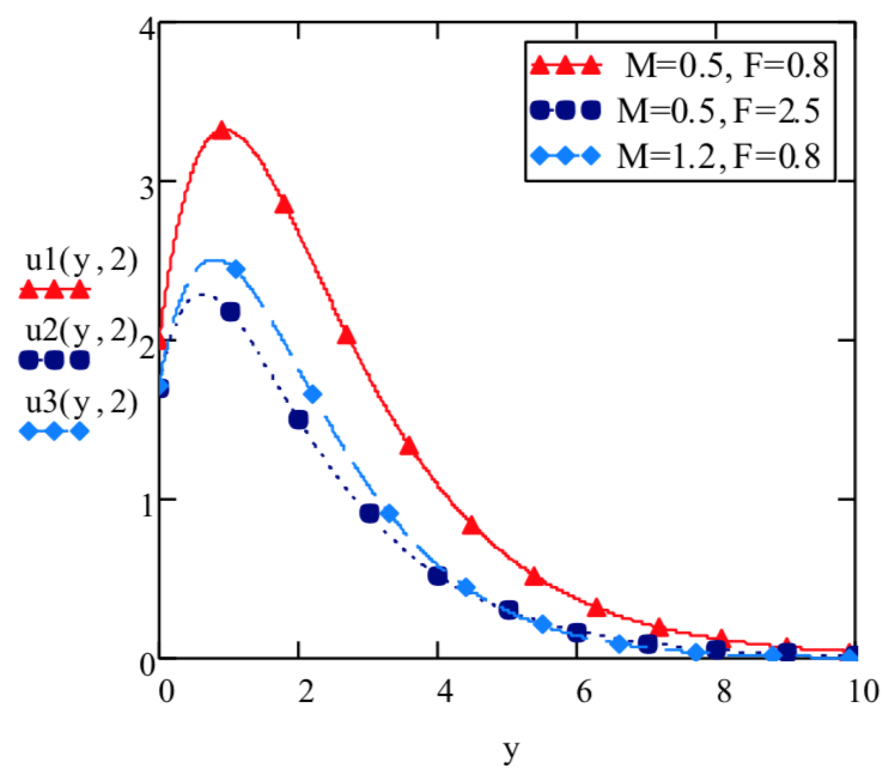
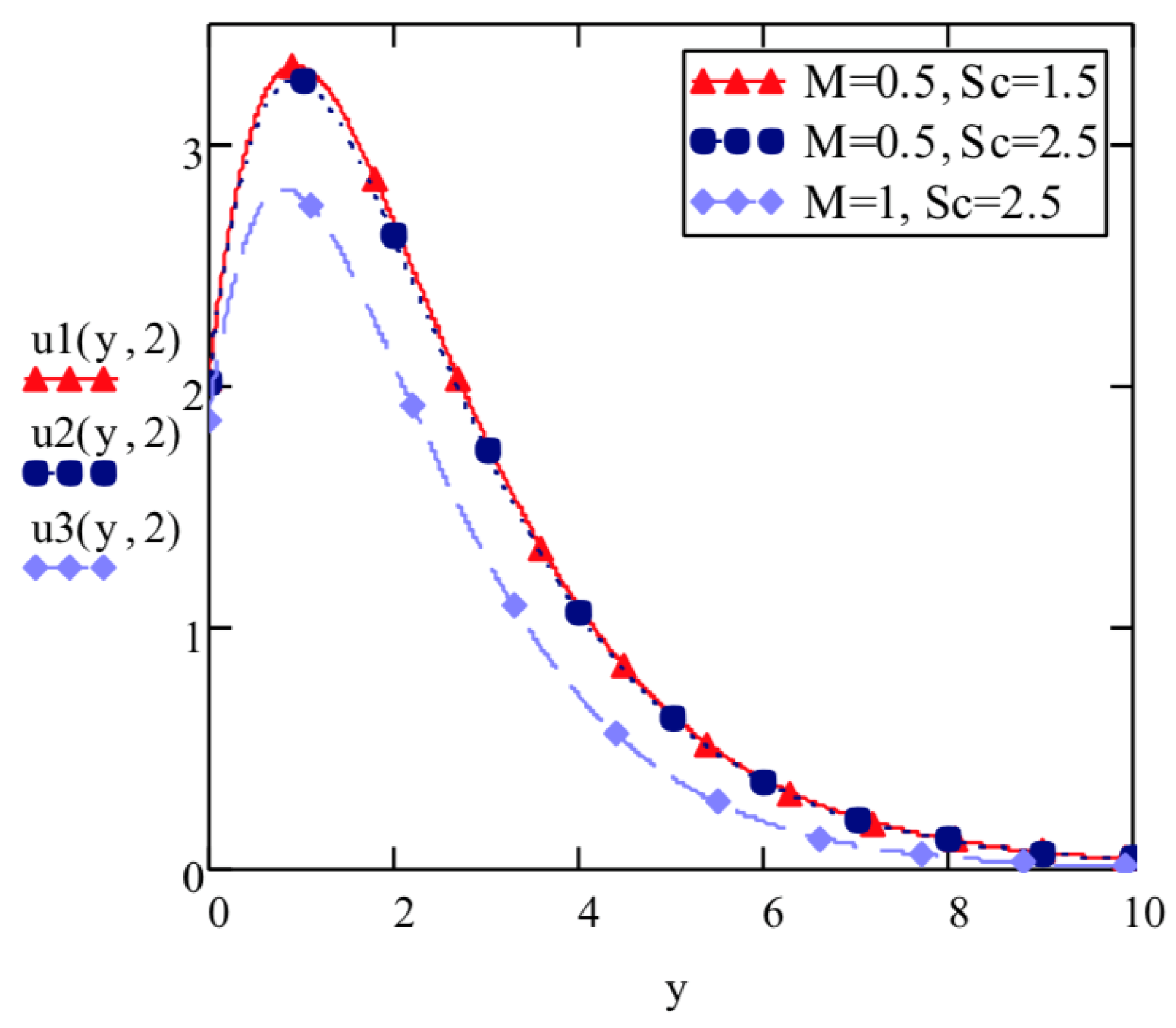
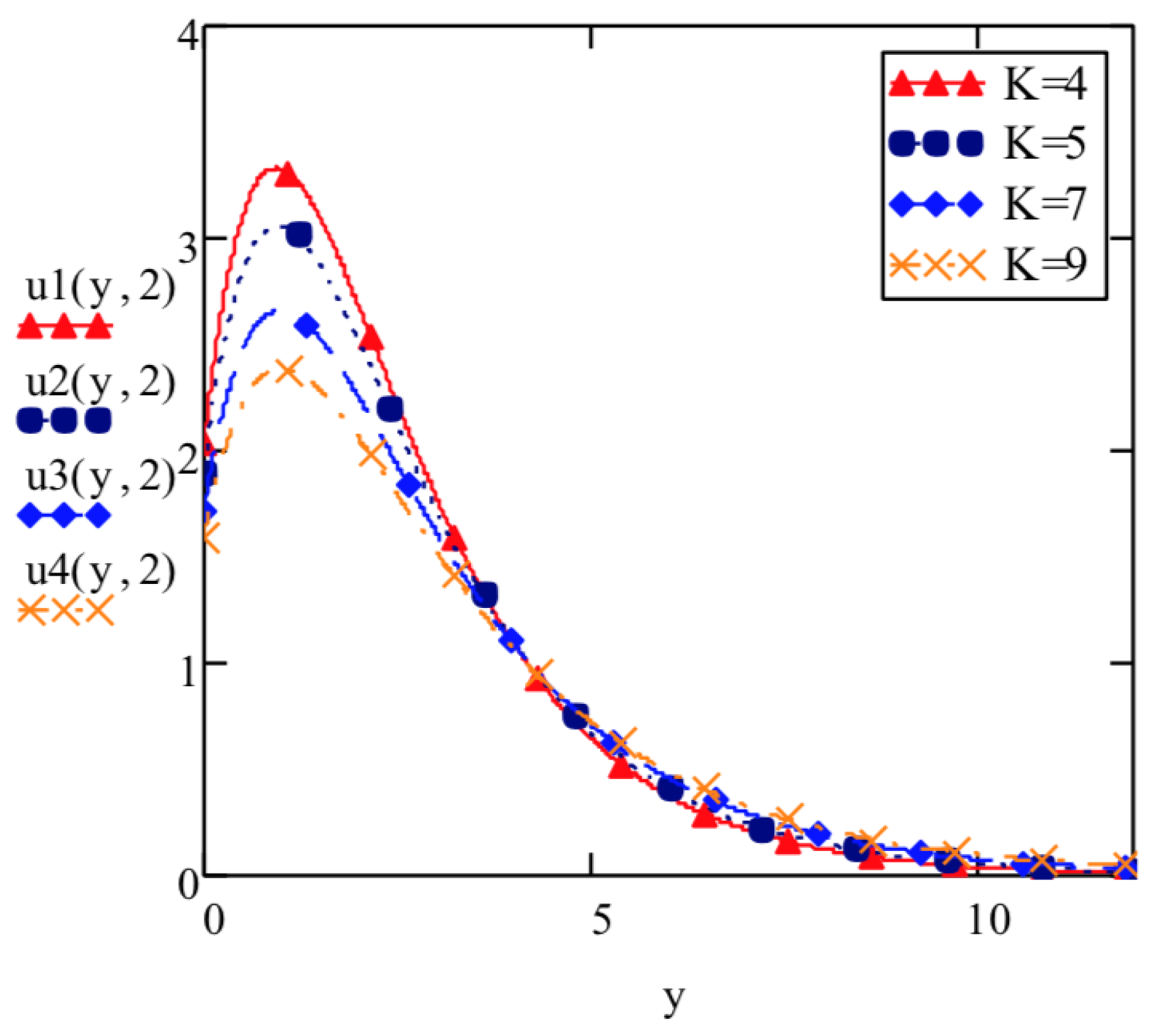
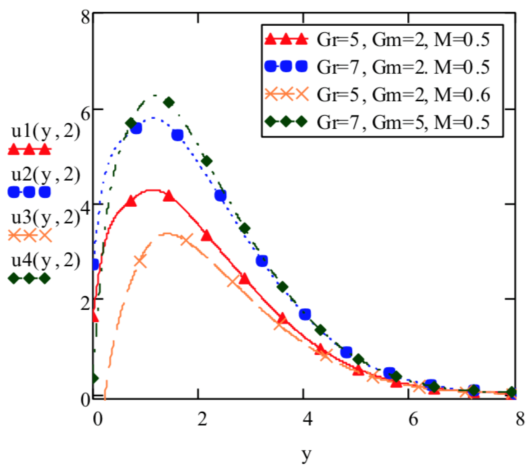
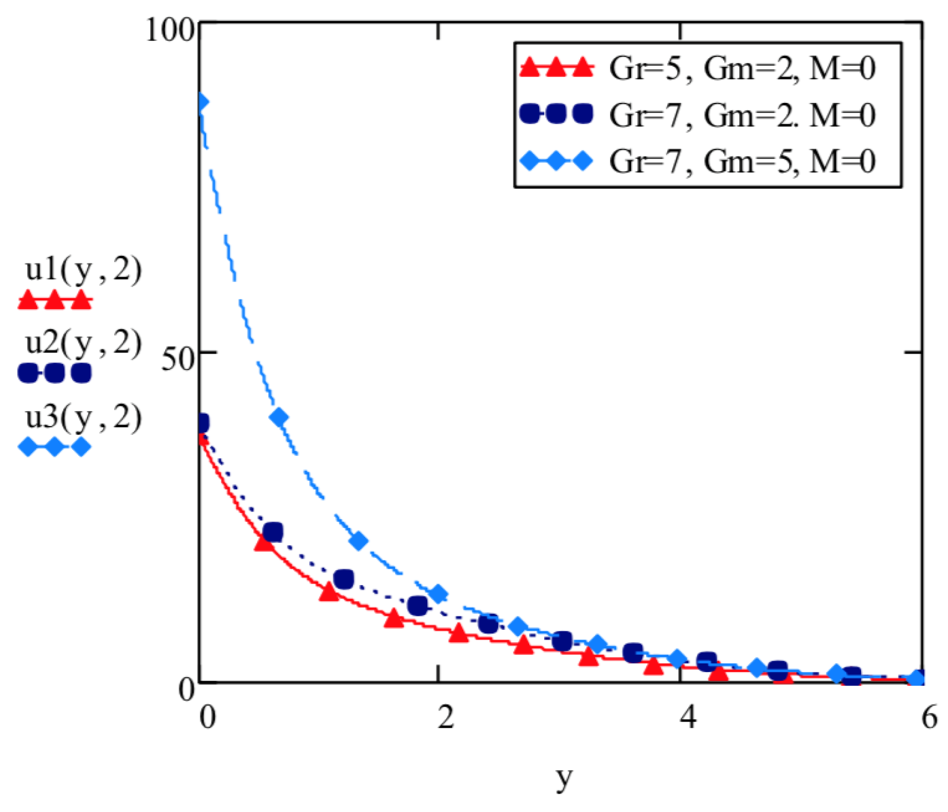
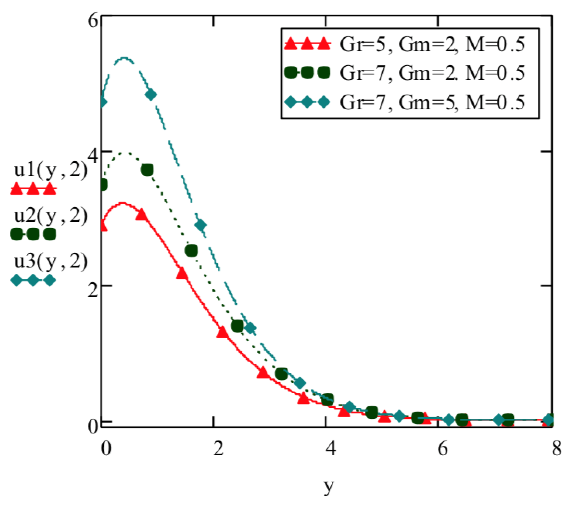
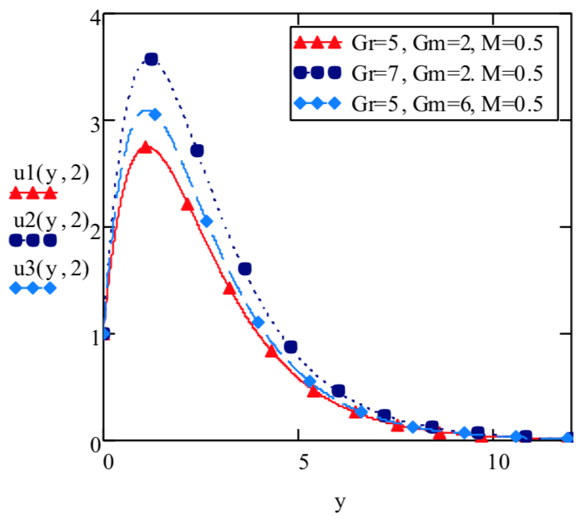
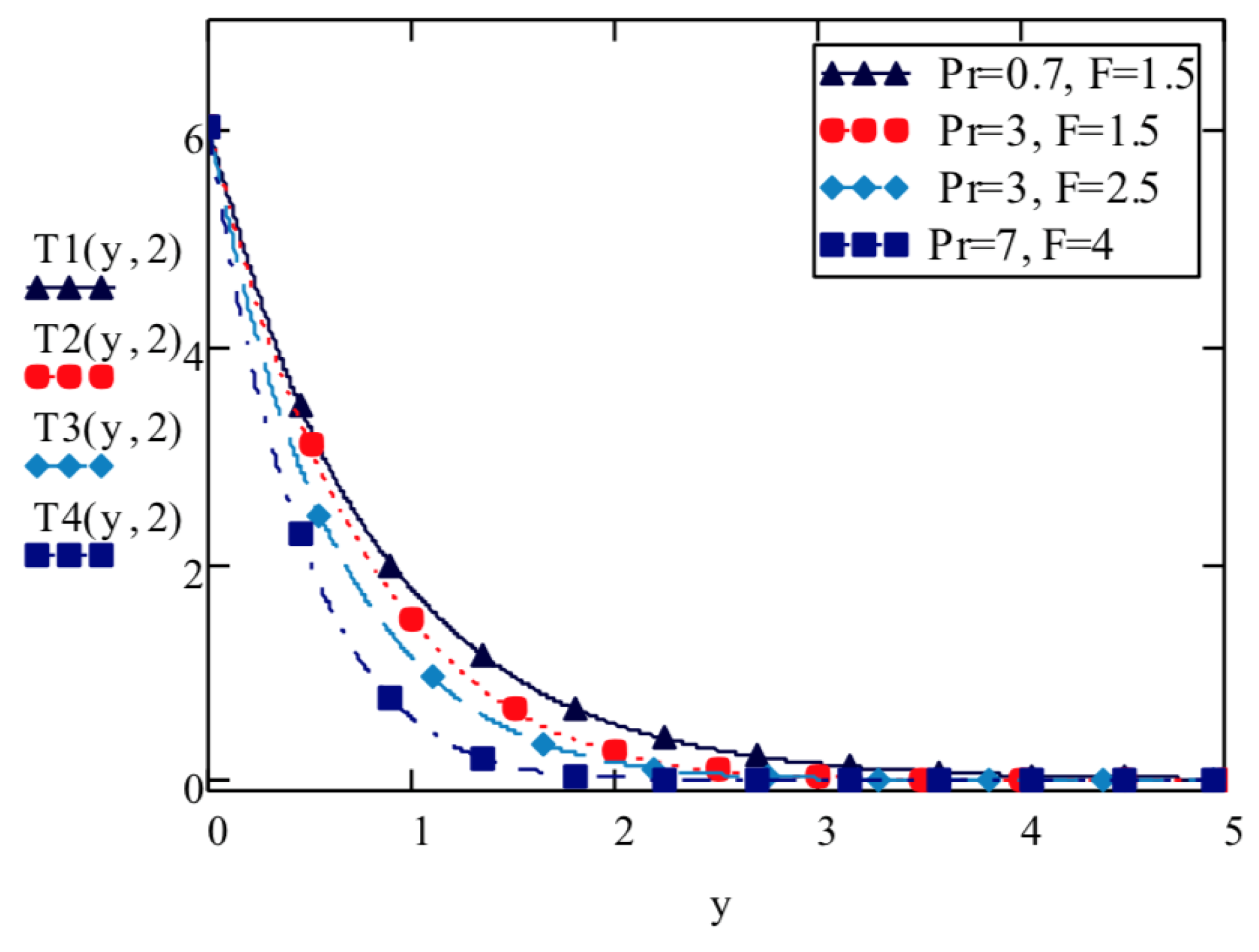
The expression of elasto-viscous fluid velocity field for the case of no-slip between fluid and plate has also been calculated. By considering $\gamma =0$ in Equation (14), we obtain $\overline{u}(y,q)$ as following

$$\begin{array}{cc}\hfill \overline{u}(y,q)=& \frac{e^{-\sqrt{\frac{q+M}{1+Kq}}y}}{q}+\frac{G_r{e}^{-\sqrt{\frac{q+M}{1+Kq}}y}}{P_{r}Kq[{(q-d)}^2-{\left(\sqrt{c}\right)}^2]}+\frac{a{G}_{r}F\left(q\right)e^{-\sqrt{\frac{q+M}{1+Kq}}y}}{P_{r}K[{(q-d)}^2-{\left(\sqrt{c}\right)}^2]}+\frac{G_m{e}^{-\sqrt{\frac{q+M}{1+Kq}}y}}{S_{c}K{q}^2[{(q-h)}^2-{\left(\sqrt{l}\right)}^2]}\hfill \\ & -\frac{G_r{e}^{-\sqrt{P_r(q+\alpha )}y}}{P_{r}Kq[{(q-d)}^2-{\left(\sqrt{c}\right)}^2]}-\frac{a{G}_{r}F\left(q\right)e^{-\sqrt{P_r(q+\alpha )}y}}{P_{r}K[{(q-d)}^2-{\left(\sqrt{c}\right)}^2]}-\frac{G_m{e}^{-\sqrt{S_{c}q}y}}{S_{c}K{q}^2[{(q-h)}^2-{\left(\sqrt{l}\right)}^2]}.\hfill \end{array}$$

(32)

For the Inverse Laplace transform, we write Equation (32) in a more simplified form

$$\begin{array}{cc}\hfill \overline{u}(y,q)=& Z_1(y,q)\frac{1}{q}+\frac{G_r}{P_{r}K}{Z}_1(y,q)\frac{1}{q[{(q-d)}^2-{\left(\sqrt{c}\right)}^2]}+\frac{G_{r}a}{P_{r}K}{Z}_1(y,q)F\left(q\right)\frac{1}{[{(q-d)}^2-{\left(\sqrt{c}\right)}^2]}\hfill \\ & +\frac{G_m}{S_{c}K}{Z}_1(y,q)\frac{1}{q^2[{(q-h)}^2-{\left(\sqrt{l}\right)}^2]}-\frac{G_r}{P_{r}K}{e}^{-\sqrt{P_r(q+\alpha )}y}\frac{1}{q[{(q-d)}^2-{\left(\sqrt{c}\right)}^2]}\hfill \\ & -\frac{a{G}_r}{P_{r}K}{e}^{-\sqrt{P_r(q+\alpha )}y}F\left(q\right)\frac{1}{[{(q-d)}^2-{\left(\sqrt{c}\right)}^2]}-\frac{G_m}{S_{c}K}{e}^{-\sqrt{S_c}y}\frac{1}{q^2[{(q-h)}^2-{\left(\sqrt{l}\right)}^2]},\hfill \end{array}$$

(33)

where

$$Z_1(y,q)=e^{-\sqrt{\frac{q+M}{1-Kq}}y}.$$

The Inverse Laplace of Equation (33) using (A1), (A2) and (A5) gives

$$\begin{array}{cc}\hfill u(y,t)=& \left(\frac{P_{r}K+(d^2-c)G_r}{P_{r}K(d^2-c)}+\frac{2G_{m}h}{S_{c}K{(h^2-l)}^2}\right){\int }_0^t{z}_1(y,s)ds\hfill \\ & +\frac{G_r}{2P_{r}K(c+d\sqrt{c})}{\int }_0^t{z}_1(y,s)e^{(d+\sqrt{c})(t-s)}ds\hfill \\ & +\frac{G_r}{2P_{r}K(c-d\sqrt{c})}{\int }_0^t{z}_1(y,s)e^{(d-\sqrt{c})(t-s)}ds+\frac{a{G}_r}{2P_{r}K\sqrt{c}}{\int }_0^t{z}_1(y,s)H_1(t-s)ds\hfill \\ & -\frac{a{G}_r}{2P_{r}K\sqrt{c}}{\int }_0^t{z}_1(y,s)H_2(t-s)ds+\frac{G_m}{S_{c}K(h^2-l)}{\int }_0^t{z}_1(y,s)(t-s)ds\hfill \\ & +\frac{G_m}{S_{c}K\left[2\sqrt{l}{(h+\sqrt{l})}^2\right]}{\int }_0^t{z}_1(y,s)e^{(h+\sqrt{l})(t-s)}ds\hfill \\ & -\frac{G_m}{S_{c}K\left[2\sqrt{l}{(h-\sqrt{l})}^2\right]}{\int }_0^t{z}_1(y,s)e^{(h-\sqrt{l})(t-s)}ds\hfill \\ & -\frac{G_r}{2P_{r}K(d^2-c)}\left[e^{y\sqrt{\alpha P_r}}erfc\left(\frac{\sqrt{P_r}y}{2\sqrt{t}}+\sqrt{\alpha t}\right)+e^{-y\sqrt{\alpha P_r}}erfc\left(\frac{\sqrt{P_r}y}{2\sqrt{t}}-\sqrt{\alpha t}\right)\right]\hfill \\ & -\frac{G_r{e}^{(d+\sqrt{c})t}}{4P_{r}K(c+d\sqrt{c})}[e^{y\sqrt{P_r(\alpha +d+\sqrt{c})y}}erfc\left(\frac{\sqrt{P_r}y}{2\sqrt{t}}+\sqrt{(\alpha +d+\sqrt{c})t}\right)\hfill \\ & +e^{-y\sqrt{P_r(\alpha +d+\sqrt{c})y}}erfc\left(\frac{\sqrt{P_r}y}{2\sqrt{t}}-\sqrt{(\alpha +d+\sqrt{c})t}\right)]\hfill \\ & -\frac{G_r{e}^{(d-\sqrt{c})t}}{4P_{r}K(c-d\sqrt{c})}[e^{y\sqrt{P_r(\alpha +d-\sqrt{c})y}}erfc\left(\frac{\sqrt{P_r}y}{2\sqrt{t}}+\sqrt{(\alpha +d-\sqrt{c})t}\right)\hfill \\ & +e^{-y\sqrt{P_r(\alpha +d-\sqrt{c})y}}erfc\left(\frac{\sqrt{P_r}y}{2\sqrt{t}}-\sqrt{(\alpha +d-\sqrt{c})t}\right)]\hfill \\ & -\frac{a{G}_{r}y}{4K\sqrt{c{P}_r}}{\int }_0^t\frac{e^{\frac{P_r{y}^2}{4s}-\alpha s}}{\sqrt{\pi s^3}}{H}_1(t-s)ds+\frac{a{G}_{r}y}{4K\sqrt{c{P}_r}}{\int }_0^t\frac{e^{\frac{P_r{y}^2}{4s}-\alpha s}}{\sqrt{\pi s^3}}{H}_2(t-s)ds\hfill \\ & -\frac{G_m{e}^{(h+\sqrt{l})t}}{4S_{c}K\sqrt{l}{(h+\sqrt{l})}^2}[e^{y\sqrt{S_c(h+\sqrt{l})y}}erfc\left(\frac{\sqrt{S_c}y}{2\sqrt{t}}+\sqrt{(h+\sqrt{l})t}\right)\hfill \\ & +e^{-y\sqrt{S_c(h+\sqrt{l})y}}erfc\left(\frac{\sqrt{S_c}y}{2\sqrt{t}}-\sqrt{(h+\sqrt{l})t}\right)]\hfill \\ & +\frac{G_m{e}^{(h-\sqrt{l})t}}{4S_{c}K\sqrt{l}{(h-\sqrt{l})}^2}[e^{y\sqrt{S_c(h-\sqrt{l})y}}erfc\left(\frac{\sqrt{S_c}y}{2\sqrt{t}}+\sqrt{(h-\sqrt{l})t}\right)\hfill \\ & +e^{-y\sqrt{S_c(h-\sqrt{l})y}}erfc\left(\frac{\sqrt{S_c}y}{2\sqrt{t}}-\sqrt{(h-\sqrt{l})t}\right)]\hfill \\ & -\frac{G_m[2h+(h^2-l)t]}{S_{c}K{(h^2-l)}^2}erfc\left(\frac{\sqrt{S_c}y}{2\sqrt{t}}\right)+\frac{G_{m}y}{2K\sqrt{S_c}(h^2-l)}{\int }_0^t\frac{e^{-\frac{S_c{y}^2}{4s}}}{\sqrt{\pi s}}ds,\hfill \end{array}$$

(34)

where

$$\begin{array}{c}\hfill z_1(y,t)=L^{-1}\left\{Z_1(y,q)\right\}=L^{-1}\left\{\left(Q_{1}oW\right)\left(q\right)\right\}=L^{-1}\left\{Q_1\left(W\left(q\right)\right)\right\}={\int }_0^{\infty }{q}_1(y,z)p(z,t)dz,\end{array}$$

$$Q_1(y,q)=e^{-\sqrt{q}y},W\left(q\right)=\frac{q+M}{1+Kq},\mathcal{N}=\frac{z(MK+1)}{K^2},$$

$$p(z,t)=L^{-1}\left\{e^{-zW\left(q\right)}\right\}=e^{\frac{z}{K}}\left[\sqrt{\frac{\mathcal{N}}{t}}{I}_1\left(2\sqrt{\mathcal{N}}t\right)e^{\frac{t}{K}}+\delta \left(t\right)\right],$$

and

$$q_1(y,t)=L^{-1}\left\{Q_1(y,q)\right\}=\frac{y}{2\sqrt{\pi t^3}}{e}^{-\frac{y^2}{4t}}.$$

5. Discussion

Figure 2 has been drawn to reflect the behaviour of elasto-viscous fluid velocity corresponding to fixed values of $G_r=5$, $G_m=2$, $P_r=0.7$, $S_c=1.5$, $M=0.5$, $F=0.8$, $\gamma =0.3$, $\alpha =1.14$, $a=5$ and $K=4$ against y at a certain time. The frequency of sine-oscillations ($f\left(t\right)=sin\left(\omega t\right)$) has been chosen as $\omega =2$. Initially, the velocity increases and then it starts decreasing, approaching zero at gaining height, thus meeting the boundary condition of velocity (8).

The response of velocity against y corresponding to parameters $G_r$, $G_m$, $S_c$, M and F has been depicted in Figure 3, Figure 4, Figure 5 and Figure 6, keeping the fixed values of $P_r$, $\gamma$, $\alpha$, a and K as above. Two cases of function $f\left(t\right)$ in condition (6) have been chosen. For a constant $f\left(t\right)$, it is observed that the velocity for elasto-viscous fluid increases with an increase in thermal Grashof number, $G_r$ and mass Grashof number, $G_m$ but decreases with an increase in Hartmann number, M. The increase in velocity due to increasing $G_r$ and $G_m$ owes its occurrence to the empowering role of conduction and mass movement of particles over resistance caused by viscous forces. These graphs also validate the physical understanding of our model that supplementary force applied on plate increases mass and thermal diffusivity near the boundary, thus increasing the thermal Grashof number, $G_r$ and mass Grashof number, $G_m$. The increased turbulence near boundary causes the velocity of fluid to rise. Also, the hindering effects of magnetic field’s presence in elasto-viscous fluid is evident through the inverse relation of fluid velocity and Hartmann number. Comparing Figure 3 and Figure 4, the elasto-viscous fluid velocity attains higher magnitude for the case of $f\left(t\right)=1$ as compared to the case of oscillating function ($\omega =2$). However, the parametric influence of $G_r$, $G_m$ and M remains unchanged for both cases.

Figure 5 and Figure 6 reflect on the influence of parameters Schmidth number, $S_c$, Hartmann number, M and thermal radiation parameter, F. It is noted that elasto-viscous fluid velocity decreases with increase in $S_c$, M and F. The smooth flow over plate is hindered by applied magnetic forces and collective movement of particles, causing a decline in velocity. In addition to manipulation of thermal radiation and electromagnetic field in reducing the velocity as the strength of these parameters is increased, it is however noted that Schmidth number’s role in inversely influencing the velocity can be considered insignificant. This fact is displayed by almost overlapping profiles of velocity for $S_c=1.5$ and $S_c=2.5$.

How, elasto-viscous parameter, K influences the velocity of fluid flow has been described through Figure 7. The velocity profiles against y have been obtained for varying values of K at a given time, $t=2$. The observation of decrease in velocity corresponding to increasing values of K is in perfect accordance with viscous and elastic effects of fluid resisting the flow motion, causing the velocity to decrease gradually. Velocity’s inverse relation with K has been apparent through the decreasing-magnitude profiles with increasing K.

In order to validate the present results, some graphs for approximating values of fluid parameters have been developed. In Figure 8, we have obtained the velocity profiles for the case of very small elasto-viscous parameter such that these profiles correspond to curves of Newtonian fluid velocity. It is observed that similar to the case of elasto-viscous fluid, Newtonian fluid velocity is directly related with $G_r$ and $G_m$ and is inversely related with M. However, due to lesser resistance caused by viscous forces for Newtonian fluid, the magnitude of its velocity exceeds the magnitude of velocity for elasto-viscous fluid.

It has also been deduced through Figure 9 that the magnitude of velocity for Newtonian fluid without the presence of magnetic field is substantially higher than for the case where magnetic field is absent. The impact of $G_r$ and $G_m$ on fluid motion remains same for $M=0$. To understand the case of variations of velocity of elasto-viscous fluid where constant temperature is provided to the boundary of plate, we have obtained the graphs in Figure 10. These profiles have been drawn for velocity against y at a certain time and fixed magnetic field but for varying values of $G_r$ and $G_m$. Following the pattern of increase in velocity with increase in $G_r$ and $G_m$ and of inverse relation with M, the fluid velocity increases swiftly in the beginning as compared to slow increase for the case of temporal provision of temperature (Figure 4) and then it starts decreasing for higher y-values, eventually approaching to zero. Also, the overall magnitude of velocity for the case of constant temperature on boundary (Figure 10) remains higher in comparison to the case in Figure 4. Provision of time-controlled temperature on the boundary of plate restrains the mass movement and flow activity, causing the velocity of fluid to decrease in comparison to the case when temperature is being provided constantly.

Figure 11 depicts the varying velocity profiles for elasto-viscous fluid against y at a given time for the case of constant velocity on boundary. All profiles retain the previous results regarding the influence of parameters $G_r$, $G_m$ and M on velocity. However, the magnitude of velocity for the case of constant velocity on boundary is lower than the cases of temporal velocity and constant temperature provision on the boundary (Figure 4 and Figure 10). Hence the combination of additional inertial push in the form of oscillations and constant temperature on boundary induces the increase in velocity magnitude of elasto-viscous fluid.

Figure 12 has been drawn to study the impact of Prandtl number, $P_r$ and thermal radiation parameter, F on temperature. The temperature profiles have been obtained against y at the given time. The observation of decrease in temperature with increase in $P_r$ and F has been made. The phenomenon of increase in temperature due to decreasing values of $P_r$ is explained by increasing magnitude of mass diffusion and thermal emission that causes the concentrated particles’ temperature to decline. Also, how Schmidt parameter $S_c$ influences the concentration of fluid has been discussed through Figure 13. It is observed that concentration of fluid, $C(y,t)$ increases with decreasing values of $S_c$ at a given time and vice-versa. Increasing Schmidt number causes mass diffusion to increase, thus lowering the mass concentration. Both Figure 12 and Figure 13 validate the facts of zero temperature and mass concentration attained at higher y-values.

To substantiate the accuracy of our analytical solutions, we have obtained the numerical results for concentration. Numerical values of concentration have been obtained using Stehfest’s algorithm [46] for calculating the Inverse Laplace transform of Equation (18). In fact, these values have been generated by making $\gamma \to 1$ in (Equation (3.1)) [36]. These numerical values have been compared with the values of concentration calculated from Equation (19) for $n=55$ terms. The computations presented in

Table 1. Values of concentration $C(y,t)$ resulting from the analytic solution Equation (19) and the numerical algorithm applied to Equation (17) at t = 5, $Sc$ = 1.

y	$\mathit{C}(\mathit{y},\mathit{t})$—Equation (19)	$\mathit{C}(\mathit{y},\mathit{t})$—Equation (17)	$\mathbf{Absolute}\mathbf{Error}$
0	5	5.00001	$6.031\times {10}^{-6}$
0.1	4.66656	4.66658	$1.694\times {10}^{-5}$
0.2	4.35403	4.35404	$1.338\times {10}^{-5}$
0.3	4.06119	4.0612	$3.346\times {10}^{-6}$
0.4	3.7869	3.78691	$6.425\times {10}^{-6}$
0.5	3.53007	3.53008	$5.33\times {10}^{-6}$
0.6	3.28967	3.28968	$4.329\times {10}^{-6}$
0.7	3.06472	3.06473	$6.388\times {10}^{-7}$
0.8	2.8543	2.8543	$5.092\times {10}^{-6}$
0.9	2.65753	2.65754	$6.509\times {10}^{-6}$
1	2.47359	2.47359	$2.626\times {10}^{-6}$

have been remarkably similar to numerical values in [36]. Stehfest’s algorithm is defined by the following relation

$$C(y,t)=L^{-1}\left\{\overline{C}(y,q)\right\}\approx \frac{ln2}{t}\sum _{k=1}^{2r}{b}_k\overline{C}\left(y,k\frac{ln2}{t}\right),$$

(35)

where r is a positive integer,

$$b_k={(-1)}^{k+r}\sum _{s=\left[\frac{k+1}{2}\right]}^{min(k,r)}\frac{s^r\left(2s\right)!}{(r-s)!s!(s-1)!(k-s)!(2s-k)!}$$

(36)

and $\left[p\right]$ denotes the integer part of the real number p. Table 1 [36] indicates the accuracy of analytical results up to the order of ${10}^{-6}$, thus authenticating our solutions of concentration. Similarly, the results of velocity and temperature can be validated.

6. Conclusions

Exact expressions of velocity, temperature and mass concentration of elasto-viscous fluid past an infinite plate have been calculated using Laplace and inverse-Laplace transform. It has been deduced that provision of temperature to the boundary of plate in non-temporal pattern and a choice of slip parameter increases fluid velocity in the presence of magnetic field of specific strength. The following salient points of current flow model have been accumulated:

• Unlike the usual adoption of numerical solutions approach for elasto-viscous fluid models, exact closed-form solutions of velocity, temperature and mass concentration have been determined and have shown to meet initial and boundary conditions.
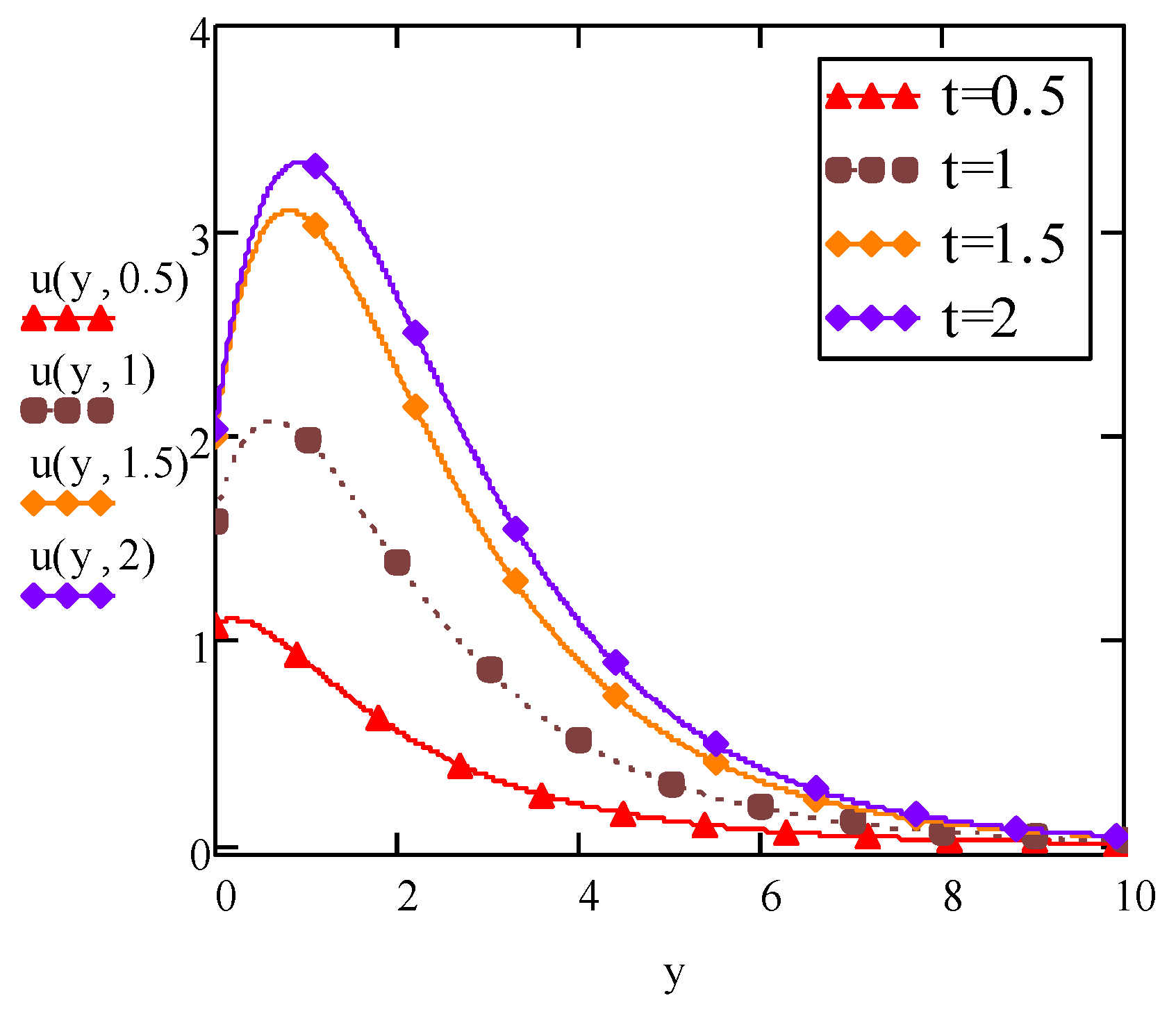
• Expressions of velocity for no-slip and timed provision of temperature on boundary were obtained. An observation of slip-parameter’s strength and temporal temperature boundary condition hindering the speed of flow was substantiated through graphical analysis.
• Validation of current results was approached through retrieving Newtonian fluid velocity expression and graphical profiles by considering very small value of elasto-viscous parameter ($K\to 0$).
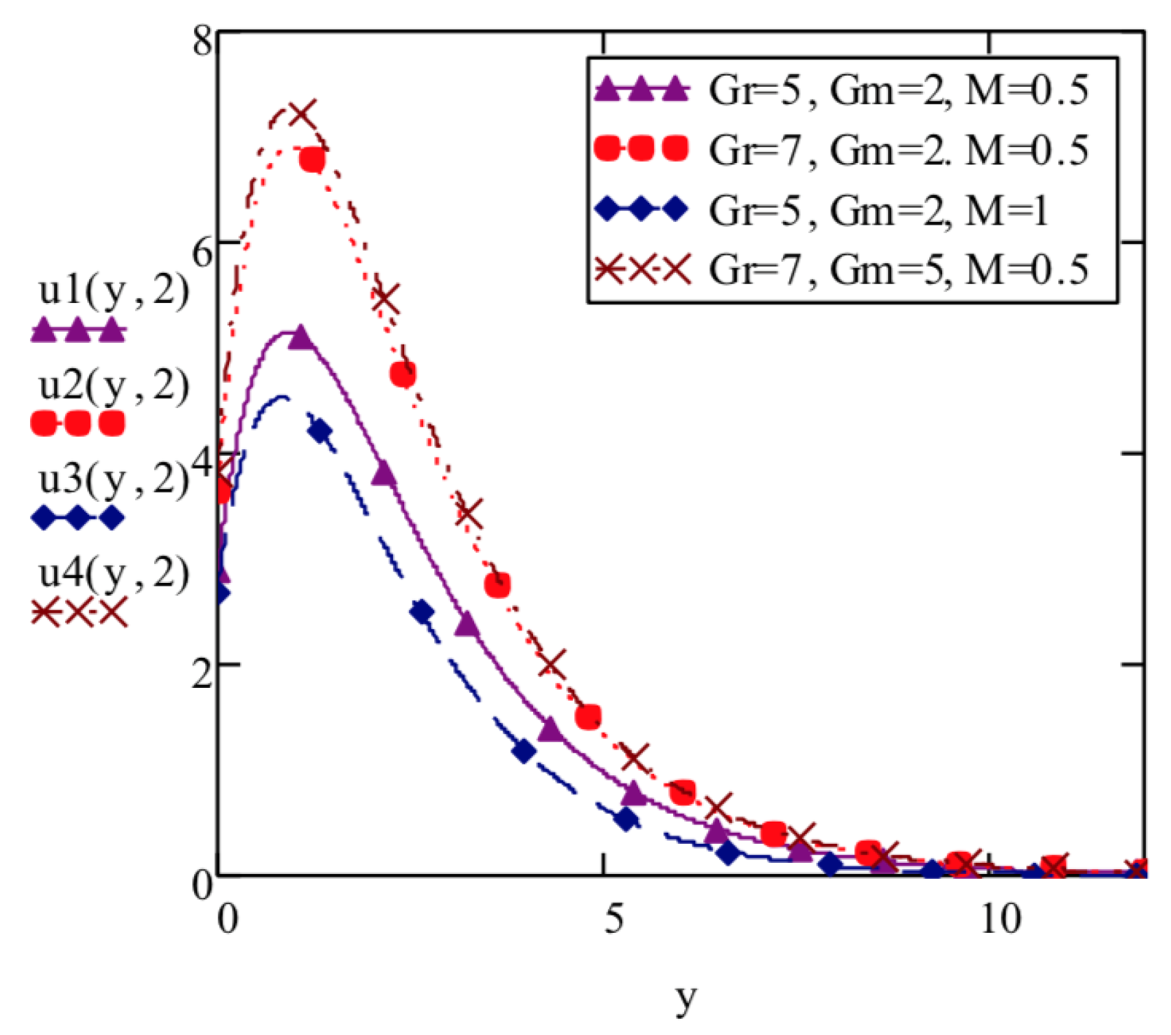
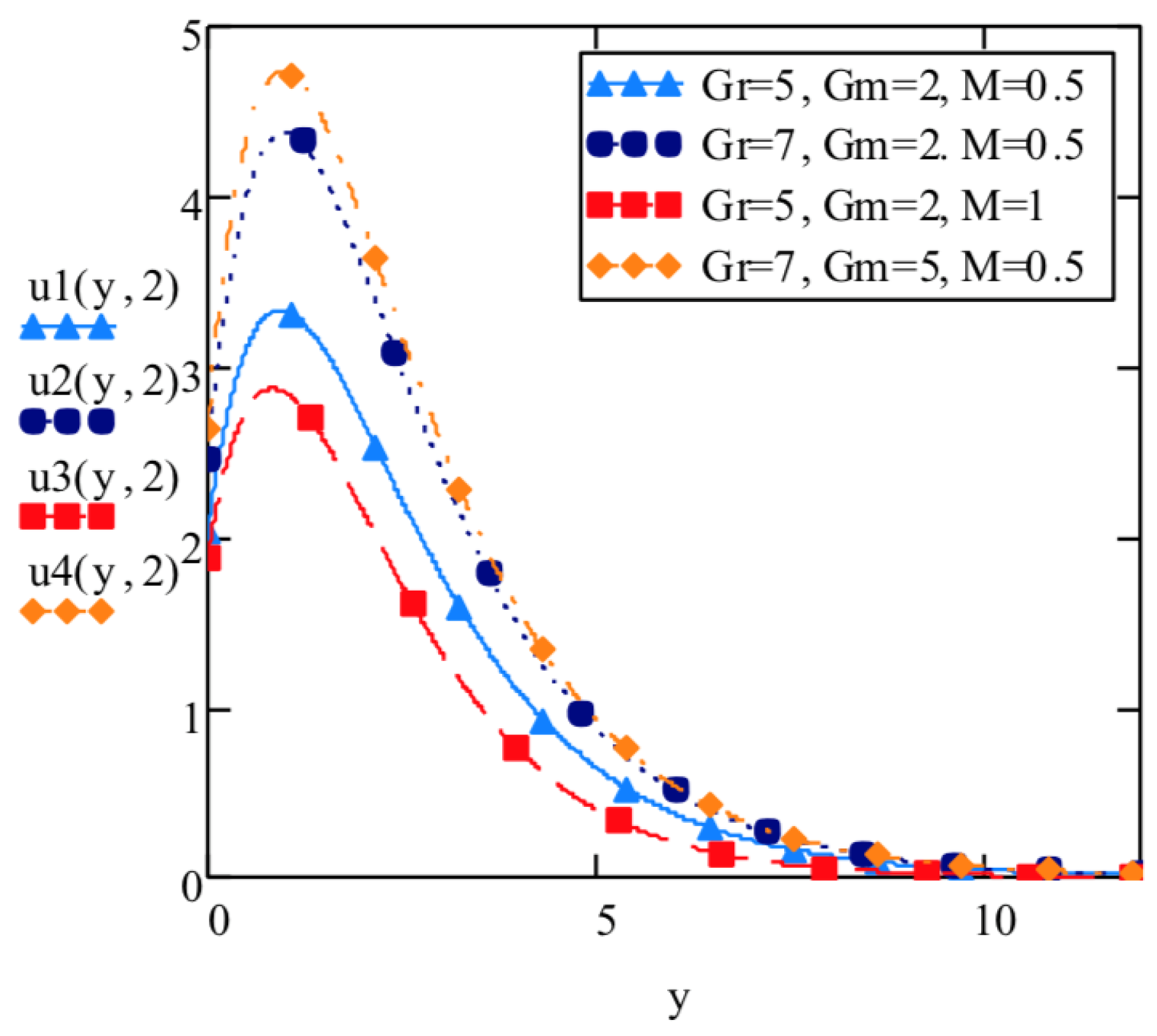
• Elasto-viscous fluid velocity increases with increase in thermal Grashof number $G_r$ and mass Grashof number $G_m$ and decreases with increase in Prandtl number $P_r$, Schmidt number $S_c$, Hartmann number M and thermal radiation parameter F.
• Temperature of fluid is inversely related with F and $P_r$.
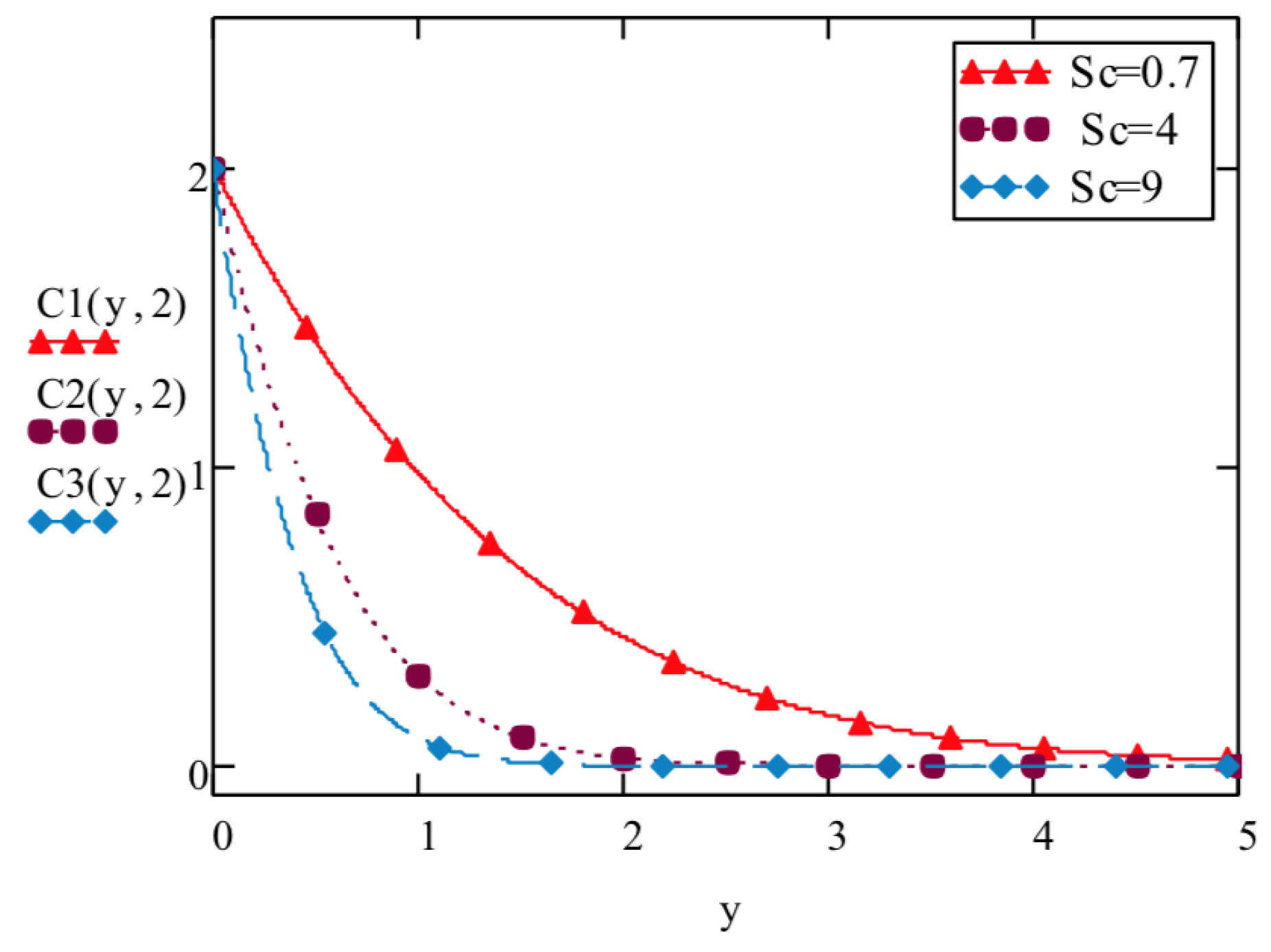
• Mass concentration of fluid increases with decrease in $S_c$ and vice-versa.
• Increasing the strength of elatso-viscous parameter K hinders the smooth flow as would be suggested by empowered viscous forces and thus decreases the flow velocity and vice-versa.
• To validate the accuracy of analytical expressions, we have generated numerical solutions for concentration of fluid. The comparison of analytical and numerical solutions points to an absolute error of order ${10}^{-6}$.

References

1. Abraham, F.; Behr, M.M.H. Shape optimization in steady blood flow: A numerical study of non-Newtonian effects. Comput. Methods Biomech. Biomed. Eng. 2005, 8, 127–137. [Google Scholar] [CrossRef] [Green Version]
2. Boghosian, M.; Cassel, K.; Hammes, M.; Funaki, B.; Kim, S.; Qian, X.; Wang, X.; Dhar, P.; Hines, J. Hemodynamics in the cephalic arch of a brachiocephalic fistula. Med. Eng. Phys. 2014, 36, 822–830. [Google Scholar] [CrossRef]
3. Ersoy, H.V. MHD Flow of a Second Order/Grade Fluid Due to Noncoaxial Rotation of a Porous Disk and the Fluid at Infinity. Math. Comput. Appl. 2010, 15, 354–363. [Google Scholar] [CrossRef] [Green Version]
4. Srinivasacharya, D.; Mendu, U. Thermal radiation and chemical reaction effects on magnetohydrodynamic free convection heat and mass transfer in a micropolar fluid. Turk. J. Eng. Environ. Sci. 2014, 38, 184–196. [Google Scholar]
5. Zhang, C.; Zheng, L.; Zhang, X.; Chen, G. MHD flow and radiation heat transfer of nanofluids in porous media with variable surface heat flux and chemical reaction. Appl. Math. Model. 2015, 39, 165–181. [Google Scholar] [CrossRef]
6. Zeeshan, A.; Ijaz, N.; Abbas, T.; Ellahi, R. The sustainable characteristic of Bio-bi-phase flow of peristaltic transport of MHD Jeffery fluid in human body. Sustainability 2018, 10, 2671. [Google Scholar] [CrossRef]
7. Samad, M.A.; Mohebujjaman, M. MHD heat and mass transfer free convection flow along a vertical stretching sheet in presence of magnetic field with heat Generation. Res. J. Appl. Sci. Eng. Tech. 2009, 1, 98–106. [Google Scholar]
8. Khaleque, S.T.; Samad, M.A. Effects of radiation, heat generation and viscous dissipation on MHD free convection flow along a stretching sheet. Res. J. Appl. Sci. Eng. Tech. 2010, 2, 368–377. [Google Scholar]
9. Zahan, I.; Samad, M.A. Radiative heat and mass transfer of an MHD free convection flow along a stretching sheet with chemical reaction, heat generation and viscous dissipation. Dhaka Univ. J. Sci. 2010, 61, 27–34. [Google Scholar] [CrossRef]
10. Uddi, Z.; Kumarb, M. MHD heat and mass transfer free convection flow near the lower stagnation point of an isothermal cylinder imbedded in porous domain with the presence of radiation. Jord. J. Mech. Ind. Eng. 2011, 5, 133–138. [Google Scholar]
11. Huang, C.; Zhang, Y. Calculation of high-temperature insulation parameters and heat transfer behaviors of multilayer insulation by inverse problems method. Chin. J. Aeronaut. 2014, 27, 791–796. [Google Scholar] [CrossRef] [Green Version]
12. Rashid, M.M.; Rostami, B.; Freidoonimehr, N.; Abbasbandy, S. Free convective heat and mass transfer for MHD fluid flow over a permeable vertical stretching sheet in the presence of the radiation and buoyancy effects. Ain Shams Eng. J. 2014, 5, 901–912. [Google Scholar] [CrossRef]
13. Seth, G.S.; Hussain, S.M.; Sarkar, S. Hydromagnetic natural convection flow with heat and mass transfer of a chemically reacting and heat absorbing fluid past an accelerated moving vertical plate with ramped temperature and ramped surface concentration through a porous medium. J. Egypt. Math. Soc. 2015, 23, 197–207. [Google Scholar] [CrossRef] [Green Version]
14. Wu, L. Mass transfer induced slip effect on viscous gas flows above a shrinking/stretching sheet. Int. J. Heat Mass Transf. 2015, 93, 17–22. [Google Scholar] [CrossRef]
15. Nayak, M.K.; Dash, G.C.; Singh, L.P. Unsteady radiative MHD free convective flow and mass transfer of a viscoelastic fluid past an inclined porous plate. Arab. J. Sci. Eng. 2015, 40, 3029–3039. [Google Scholar] [CrossRef]
16. Dawar, A.; Shah, Z.; Idrees, M.; Khan, W.; Islam, S.; Gul, T. Impact of Thermal Radiation and Heat Source/Sink on Eyring–Powell Fluid Flow over an Unsteady Oscillatory Porous Stretching Surface. Math. Comput. Appl. 2018, 23, 20. [Google Scholar] [CrossRef]
17. Ellahi, R.; Alamri, S.Z.; Basit, A.; Majeed, A. Effects of MHD and slip on heat transfer boundary layer flow over a moving plate based on specific entropy generation. J. Taibah Univ. Sci. 2018, 12, 476–482. [Google Scholar] [CrossRef]
18. Yildiz, B.; Kazimi, M.S. Efficiency of hydrogen production systems using alternative nuclear energy technologies. Int. J. Hydrog. Energy 2006, 31, 77–92. [Google Scholar] [CrossRef]
19. Bhatti, M.M.; Abbas, T.; Rashidi, M.M.; Ali, M.; Yang, Z. Entropy generation on MHD Eyring–Powell nanofluid through a permeable stretching surface. Entropy 2016, 18, 224. [Google Scholar] [CrossRef]
20. Hussain, F.; Ellahi, R.; Zeeshan, A. Mathematical models of electro-magnetohydrodynamic multiphase flows synthesis with nano-sized hafnium particles. Appl. Sci. 2018, 8, 275. [Google Scholar] [CrossRef]
21. Erdogan, M.E. A note on an unsteady flow of a viscous fluid due to an oscillating plane wall. Int. J. Non-Linear Mech. 2001, 35, 1–6. [Google Scholar] [CrossRef]
22. Hayat, T.; Siddiqui, A.M.; Asghar, S. Some simple flows of an Oldroyd-B fluid. Int. J. Eng. Sci. 2001, 39, 135–147. [Google Scholar] [CrossRef]
23. Fetecau, C.; Fetecau, C. Starting solutions for some unsteady unidirectional flows of a second grade fluid. Int. J. Eng. Sci. 2005, 43, 781–789. [Google Scholar] [CrossRef]
24. Fetecau, C.; Fetecau, C. Starting solutions for the motion of a second grade fluid due to longitudinal and torsional oscillations of a circular cylinder. Int. J. Eng. Sci. 2006, 44, 788–796. [Google Scholar] [CrossRef]
25. Yao, Y.; Liu, Y. Some unsteady flows of a second grade fluid over a plane wall. Nonlin. Anal. Real World Appl. 2010, 11, 4442–4450. [Google Scholar] [CrossRef]
26. Vieru, D.; Fetecau, C.; Sohail, A. Flow due to a plate that applies an accelerated shear to a second grade fluid between two parallel walls perpendicular to the plate. Z. Angew. Math. Phys. 2011, 62, 161–172. [Google Scholar] [CrossRef]
27. Fetecau, C.; Fetecau, C.; Rana, M. General solutions for the unsteady flow of second-grade fluids over an infinite plate that applies arbitrary shear to the fluid. Z. Naturforschung 2011, 66, 753–759. [Google Scholar] [CrossRef]
28. Fetecau, C.; Vieru, D.; Fetecau, C. Effect of side walls on the motion of a viscous fluid induced by an infinite plate that applies an oscillating shear stress to the fluid. Cent. Eur. J. Phys. 2011, 9, 816–824. [Google Scholar] [CrossRef] [Green Version]
29. Soundalgekar, V.M. Free convection effects on the flow past a vertical oscillating plate. Astrophys. Space Sci. 1979, 66, 165–172. [Google Scholar] [CrossRef]
30. Soundalgekar, V.M.; Akolkar, S.P. Effects of free convection currents and mass transfer on flow past a vertical oscillating plate. Astrophys. Space Sci. 1983, 89, 241–254. [Google Scholar] [CrossRef]
31. Gupta, P.S.; Gupta, A.S. Radiation Effect on hydromagnetic convection in a vertical channel. Int. J. Heat Mass Trans. 1974, 17, 1437–1442. [Google Scholar] [CrossRef]
32. Soundalgekar, V.M.; Lahurikar, R.M.; Pohanerkar, S.G.; Birajdar, N.S. Effects of mass transfer on the flow past an oscillating infinite vertical plate with constant heat flux. Thermophys. Aeromech. 1994, 1, 119–124. [Google Scholar]
33. Fetecau, C.; Rana, M.; Fetecau, C. Radiative and porous effects on free convection flow near a vertical plate that applies shear stress to the fluid. Zeitschrift für Naturforschung A 2012, 68, 130–138. [Google Scholar] [CrossRef]
34. Deka, R.K.; Neog, B.C. Combined effects of thermal radiation and chemical reaction on free convection flow past a vertical plate in porous medium. Adv. Appl. Fluid Mech. 2009, 6, 181–195. [Google Scholar]
35. Shahid, N. A study of heat and mass transfer in a fractional MHD flow over an infinite oscillating plate. SpringerPlus 2015, 4, 640. [Google Scholar] [CrossRef]
36. Shahid, N. Effects of thermal radiation and mass diffusion on MHD flow over a vertical plate applying time-dependent shear to the fluid. Neural Parallel Sci. Comput. 2016, 24, 431–452. [Google Scholar]
37. Singh, A.K.; Singh, A.K.; Singh, N.P. Heat and mass transfer in MHD flow of a viscous fluid past a vertical plate under oscillatory suction velocity. Indian J. Pure Appl. Math. 2003, 34, 429–433. [Google Scholar]
38. Chen, C.H. Combined heat and mass transfer in MHD free convection from a vertical surface with Ohmic heating and viscous dissipation. Int. J. Eng. Sci. 2004, 42, 699–713. [Google Scholar] [CrossRef]
39. Aboeldahab, E.M.; Elbarbary, E.M.E. Hall current effect magneto-hydrodynamics free convection flow past a semi.-infinite vertical plate with mass transfer. Int. J. Eng. Sci. 2001, 39, 1641–1652. [Google Scholar] [CrossRef]
40. Sharma, B.K.; Chaudhary, R.C. Hydromagnetic unsteady mixed convection and mass transfer flow past a vertical plate immersed in a porous medium with Hall effect. Eng. Trans. 2005, 56, 3–23. [Google Scholar]
41. Raju, R.S.; Reddy, G.J.; Rao, J.A.; Rashidi, M.M.; Gorla, R.S.R. Analytical and numerical study of unsteady MHD free convection flow over an exponentially moving vertical plate with heat absorption. Int. J. Therm. Sci. 2016, 107, 303–315. [Google Scholar] [CrossRef]
42. Rashidi, M.M.; Bagheri, S.; Momoniat, E.; Freidoonimehr, N. Entropy analysis of convective MHD flow of third grade non-Newtonian fluid over a stretching sheet. Ain Shams Eng. J. 2017, 8, 77–85. [Google Scholar] [CrossRef] [Green Version]
43. Bhatti, M.M.; Abbas, M.A.; Rashidi, M.M. A robust numerical method for solving stagnation point flow over a permeable shrinking sheet under the influence of MHD. Appl. Math. Comput. 2018, 316, 381–389. [Google Scholar] [CrossRef]
44. Shahid, N. Role of a Structural Parameter in Modelling Blood Flow Through a Tapering Channel. Bound. Value Probl. 2018, 2018, 84. [Google Scholar] [CrossRef]
45. Landau, L.D.; Llfshltz, E.M. Fluid Mechanics; Elsevier: New York, NY, USA, 1978. [Google Scholar]
46. Stehfest, H. Algorithm 368: Numerical inversion of Laplace transform. Commun. ACM 1979, 13, 47–49. [Google Scholar] [CrossRef]
Figure 1. Geometry of flow.
Mca 24 00031 g001
Figure 2. Elasto-viscous velocity versus y at varying t .
Mca 24 00031 g002
Figure 3. Elasto-viscous velocity versus y at t = 2 .
Mca 24 00031 g003
Figure 4. Elasto-viscous velocity versus y at t = 2 .
Mca 24 00031 g004
Figure 5. Elasto-viscous velocity versus y at t = 2 .
Mca 24 00031 g005
Figure 6. Elasto-viscous velocity versus y at t = 2 .
Mca 24 00031 g006
Figure 7. Elasto-viscous velocity versus y at t = 2 .
Mca 24 00031 g007
Figure 8. Newtonian fluid velocity versus y at t = 2 .
Mca 24 00031 g008
Figure 9. Newtonian fluid velocity for no-magnetic field versus y at t = 2 .
Mca 24 00031 g009
Figure 10. Newtonian fluid velocity for constant temperature on boundary versus y at t = 2 .
Mca 24 00031 g010
Figure 11. Elasto-viscous velocity for constant velocity condition on boundary versus y at t = 2 .
Mca 24 00031 g011
Figure 12. Temperature of fluid, T ( y , t ) versus y at t = 2 .
Mca 24 00031 g012
Figure 13. Mass concentration of fluid, C ( y , t ) versus y at t = 2 .
Mca 24 00031 g013