Abstract
Shape optimization is a very time-consuming and expensive task, especially if experimental tests need to be performed. To overcome the challenges of geometry optimization, the industry is increasingly relying on numerical simulations. These kinds of problems typically involve the interaction of three main applications: a solid modeler, a multi-physics solver, and an optimizer. In this manuscript, we present a shape optimization work-flow entirely based on open-source tools; it is fault tolerant and software agnostic, allows for asynchronous simulations, and has a high degree of automation. To demonstrate the usability and flexibility of the proposed methodology, we tested it in a practical case related to the naval industry, where we aimed at optimizing the shape of a bulbous bow in order to minimize the hydrodynamic resistance. As design variables, we considered the protrusion and immersion of the bulbous bow, and we used surrogate-based optimization. From the results presented, a non-negligible resistance reduction is obtainable using the proposed work-flow and optimization strategy.
1. Introduction
Engineering design and product development using shape optimization can be a very daunting task, especially if the design approach is experimental, where cost and time constraints usually limit the number of prototypes that are possible to construct and test. Moreover, it is required to have an in-depth know-how of the problem being studied to choose which configurations to analyze. In this view, the continuous development of numerical methods and the increase in computing performance have suggested the use of simulation software able to model complex multi-physics problems and optimize the design space, thereby reducing the costs related to prototypes, physical experiments, and field/operational tests.
Proprietary numerical simulation tools allow very detailed analysis, but their use often requires the acquisition of expensive licenses. An alternative to commercial software is the use of free and open-source technology (e.g., GNU General Public License, BSD license, MIT license). This type of software licensing model gives users the freedom to use, read, write, and redistribute the source code, with no price tag attached. More importantly, open-source software has the same capabilities as their commercial counterparts, and it is mature enough so that it can be used in the design and certification process of new products.
With this in mind, we address in this manuscript the implementation of an open-source framework for shape optimization. In particular, we focus our attention on fluid dynamics problems applied to ship design. Nevertheless, the same methodology can be used in any engineering field. In doing so, essentially four tasks need to be addressed:
- How to efficiently and accurately simulate the physics involved.
- How to modify the geometry or mesh.
- How to search the optimal configuration.
- How to interface the applications involved in the optimization loop.
In the context of naval architecture design, the adoption of shape optimization using numerical simulations is not new. The advantages of hull optimization and related devices optimization (such as propellers and hydrofoils) have been demonstrated by several authors. Many design optimization approaches have been used in the design of traditional propellers [1,2], unconventional propulsion systems [3,4], appendages [5], and the optimization of the entire hull shape [6,7]. Recently, a lot of development has been done on the design of unconventional vessels with special mission profiles, from the standard mono-hull shapes [8,9], to unconventional multi-hulls [10,11], or hulls with special shapes, such as the Small Waterplane Area Twin Hull or SWAT [12]. However, even if these design methods have reached a satisfactory maturity level, the hull shape optimization is still confined to the research level due to its high complexity.
One of the main drawbacks of shape optimization for complex industrial applications is the large computational times required to get the outcomes. In naval architecture design (where we are mainly interested in evaluating resistance and seakeeping, among other things), this is usually overcome by the use of highly efficient low-fidelity or medium-fidelity methods, such as the boundary element methods (BEM). However, such approaches are not able to predict the wave pattern generated by the ship, do not include viscous effects, or neglect other nonlinear behaviors (which can be important in order to obtain a proper performance prediction for certain ships). Even though successful applications with low-fidelity methods have been previously reported in the literature [10], the adoption of high-fidelity solvers (such as finite volume method or finite element method solvers) in the design loop can increase the accuracy and reliability of the design process. In this field, many studies have been conducted, for example, Serani et al. [13] successfully used a viscous solver for addressing the shape optimization of a high-speed catamaran with excellent results; however, the computational cost in terms of CPU time (for the whole optimization loop and each single simulation) and the complexity of the optimization loop was too big to be implemented by a manufacturer (particularly small ones, which have limited resources). In light of this, innovative optimization methods to simplify and speed up the entire optimization process are under investigation, such as multi-level optimization [14], surrogate-based optimization [15], proper orthogonal decomposition and dynamic mode decomposition [16], machine learning for interactive design and fluid dynamics simulations [17], data-driven simulations and optimization [18], and generative design [19].
In the shipbuilding industry, the bulbous bow shape is usually designed to reduce the ship wave-making resistance. The hull drag resistance can be split into three main contributions: the wave-making drag, the friction drag, and the wake drag. Depending on the ship speed, the contribution of each component to the total resistance value can be drastically different. Considering the present case, the wave-making component is one of the most important; therefore, its reduction by optimizing the bulbous bow shape can give a not negligible contribution to the whole design (for example, a reduction of some percentage of the fuel consumption). Following the guidelines proposed by Kracht [20], the bulbous bow shape can be defined by six non-dimensional parameters. With the goal of decreasing the computational cost by reducing the design space, and at the same time being able to represent the bulbous bow shape without losing geometrical information, only two design parameters are considered in this study. Nevertheless, the proposed approach can be extended to more complex cases where, for instance, one is interested in having more local control of the bulbous bow shape by using more design variables. Previous work addressing bulbous bow optimization using computational fluid dynamics (CFD) can be found in References [21,22,23,24,25]. The aforementioned sources show the benefits of CFD optimization, but most of them fail in explaining the importance of the application interfacing tool, automation of the loop, and real-time analytics.
Hereafter, we propose a vertical work-flow that could potentially simplify and automate the design and optimization process. All the tools used in this work are open-source, and this translates to cost savings, as no commercial licenses are used. To generate the domain mesh and to compute the hydrodynamic resistance of the hull (including the bulbous bow), we used the multi-physics solver OpenFOAM [26] (version 5.0). To create new geometry candidates, we used the free-form deformation application MiMMO [27]. To reduce the number of optimization iterations and to get an initial screening of the design space, we used surrogate-based optimization. The optimization algorithms and the code coupling interface is provided through the Dakota library [28] (version 6.7). Finally, all the real-time data analytics, quantitative post-processing, and data analytics were performed using Python and bash scripting. Previous attempts in coupling OpenFOAM and Dakota to deal with shape optimization problems are described in References [29,30,31,32,33,34,35,36], but none of them have addressed how to interface different applications in an optimization loop (besides OpenFOAM and Dakota), how to deal with concurrent simulations, work-flow automation, fault-tolerant loops, real-time data analytics, and the importance of knowledge extraction. We aim at coupling all tools needed for shape optimization studies in a streamlined work-flow, with a high degree of automation and flexibility, and using efficient optimization techniques that allow engineers to explore, exploit, and optimize the design space from a limited number of training observations.
2. Description of the Optimization Framework and Optimization Strategy
In a typical shape optimization study, many applications can live together (e.g., solid modeler, shape morpher, mesh generator, multi-physics solver, optimizer, knowledge extraction tools, coupling utilities, and so on), making the optimization loop very difficult to set up, monitor, and control. Moreover, the optimization loop must be fault tolerant, that is, in the event of an unexpected failure of the system (hardware or software), the user should be able to restart from a previously saved state. The optimizer should also be flexible, in the sense that it should provide a variety of optimization methods, design of experiment techniques, and code coupling interfaces to different simulation software and programming languages. Finally, to reduce the long execution times inherent to computational fluid dynamics (CFD) optimization studies, the optimization loop should be able to work in parallel and deploy many simulations at the same time. Furthermore, everything should be done without overwhelming the user. We aim at addressing the findings and recommendations reported in the NASA contractor report “CFD Vision 2030 Study: A Path to Revolutionary Computational Aerosciences” [37], where the authors state: “A single engineer/scientist must be able to conceive, create, analyze, and interpret a large ensemble of related simulations in a time-critical period (e.g., 24 hours), without individually managing each simulation, to a pre-specified level of accuracy”.
In this work, we successfully coupled many applications used in traditional CFD work-flows to efficiently conduct general CFD optimization studies. We used the library Dakota [28,38] as the optimizer and application interface tool. The Dakota library provides a flexible and extensible interface between simulation codes and iterative analysis methods. This library contains many gradient-based methods and derivative-free methods for design optimization studies, uncertainty quantification, and parameter estimation capabilities. Dakota also contains many design of experiment methods to conduct sensitivity studies. With Dakota, the user is not obliged to use the optimization and space exploration methods implemented on it: one can easily interface Dakota with a third-party optimization library. The library also offers restart capabilities and solution monitoring. Most important, it is software neutral, in the sense that it can interface any application that it is able to parse input/output files via a command line interface.
The optimization loop is illustrated in Figure 1. In this work-flow, the starting point is the initial geometry which is manipulated with a free-form deformation tool to generate new shapes. The MiMMO library [27], which uses radial basis functions (RBF) to shape the geometry [39,40,41,42], was used as geometry manipulation tool. With MiMMO, the user is only asked to define a series of control points, these control points are then moved in the design space, and together with the RBF function, they generate a smooth displacement field that represents the new geometry. To have more control over the deformation, the user can define a deformable region using a control box. Then, the continuity between the region to be deformed and the area labeled as undeformed is ensured by using continuous level set functions. In Figure 2, we illustrate the original geometry (left image), where we highlight the control points and the selection box used to deform the base geometry. In this figure (right image), we also show two deformed geometries. In the figure depicted, we only used one control point to deform the geometry, but more control points can be used with no problem. It is worth mentioning that in this framework, we only take one initial geometry. Then, starting from this geometry, we can generate many variations of it. In general, the shape morphing task is computationally inexpensive. We would like to emphasize that, at this point, any geometry manipulation tool can be used; the main reasons in using MiMMO are that the input files used by this library can be easily parameterized and it also offers mesh morphing capabilities (which are not discussed in this manuscript).
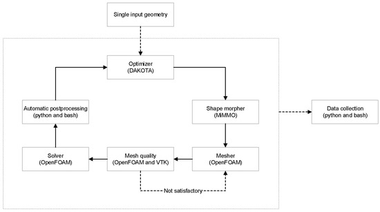
Figure 1.
Optimization loop. Notice that it only takes one single geometry. During the whole optimization loop, data are continuously collected.
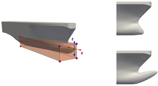
Figure 2.
Left: undeformed geometry. The green sphere represents the control point used to deform the geometry; this control point can move in the plane XZ. The surface region within the selection box is free to deform. Right: two deformed geometries.
After generating the input geometry, we can move to the meshing phase. To mesh the computational domain, we used the meshing tools distributed with the open-source OpenFOAM library [26,43], namely, blockMesh and snappyHexMesh. These tools generate high-quality hexahedral-dominant meshes and can be easily parameterized. The whole meshing process is fully automatic and, to some extent, fault tolerant. During the meshing stage, we always monitored the quality of the far-field mesh, the quality of the inflation layers close to the body, and the transition between regions with different cell sizes. In the case of mesh quality problems (such as high non-orthogonality, high skewness, too aggressive expansion ratios between cells, or discontinuous inflation layers in critical areas), the mesh was automatically recomputed using more robust predefined parameters, which generates better meshes but at the cost of a higher cell count. The meshing parameters were determined using the original geometry, and two additional geometries representing the worst case scenarios (highly deformed bulbs). The possibility of using the meshing tools in parallel and concurrently allowed us to obtain fast outcomes.
All the numerical simulations were conducted using the open-source OpenFOAM library [26,43], which is a multi-physics solver based on the cell-centered finite volume method. This library has been extensively validated, counts with a wide community, is highly scalable in parallel architectures, and the simulation setup can be easily parameterized. As soon as the optimization loop was started, the simulations did not require continuous user supervision. Several quantities of interest (QoI) were sampled during each computation, and in the case of anomalies (such as high oscillations in the forces, unbounded quantities, or mass imbalance), the simulation parameters were automatically changed to a more robust and stable discretization scheme. The default and modified solver parameters were determined after conducting an extensive validation of the solver (as explained in Section 4). All the simulations were run in parallel, and as the optimization method used did not require the computation of gradients, we were able to run many simulations concurrently. The whole framework was deployed in an out-of-the-box workstation, with 16 cores and 128 GB of RAM. As all the tools used require only publicly available compilers and libraries, the same framework can be easily deployed in distributed memory HPC architectures.
At this point, we need to define the optimization strategy. One major obstacle to the use of optimization in CFD is the long CPU times of the simulations and, depending on the method used, the need for computing gradients or the need for running a large number of simulations to obtain the design space sensitivities. Therefore, due to the long computational times and the lack of analytic gradients, optimization in CFD is a slow iterative-converging task. With this in mind, we need to choose an optimization method that is reliable, computationally affordable, and will meet our deadlines.
Gradient-based methods have good converging rates, but they require the computation of the gradients (and depending o the method used, they might require the computation of the Hessians), and in the presence of a large design space these quantities can be very expensive to compute. Gradient-based methods also require some basic knowledge of the problem, as well as some input parameters (e.g., starting point in the parameter space, bounds of the design variables, iterative and gradients tolerances, how to compute the derivatives, and so on), and they do not give much information regarding the global behavior of the design space. Additionally, they do not guarantee the convergence to a global optimal value. On the other hand, global derivative-free methods have slow convergence rates, but they are more likely to converge to the global optimal value than local methods. Also, since they do not require the computation of the gradients, they behave quite well in the presence of numerical noise. However, to reach the optimal value, they need to perform a large number of function evaluations, which can impose serious time limitations, especially if we are running unsteady CFD simulations.
Another approach to conduct optimization is the so-called surrogate-based optimization (SBO), which is the method used in this study. The SBO method consists of constructing a mathematical model (also known as a surrogate, response surface, meta-model, emulator) from a limited number of observations (CFD simulations, in our case). After building the surrogate, the optimization can be performed at this level. Furthermore, during the design space exploration process, SBO provides a better global understanding of the problem, allowing the use of exploratory data analysis techniques and machine learning methods to get more insight, discover hidden patterns, and detect anomalies in the design space. In Figure 3, we illustrate the basic work-flow of the SBO method. The work-flow is rather simple; we start by conducting a limited number of simulations (design space exploration). After gathering the information at the design points, we can use those observations to construct the mathematical model or surrogate. At this point, we can validate the surrogate by comparing the values obtained from the high-fidelity simulations against the predicted values using the surrogate, or we can refine the surrogate by adding more training points. After building, validating, and improving the meta-model, we can use any optimization method to find the optimal value. Working at the surrogate level is orders of magnitude faster than working at the high-fidelity level [44].
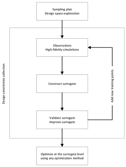
Figure 3.
Surrogate-based optimization work-flow.
It is important to mention that more sophisticated SBO techniques exist, such as efficient global optimization (EGO), gradient-enhanced meta-models, and adaptive sampling response surfaces [38,44,45,46,47]. We did not use any of those state-of-the-art SBO approaches, because we were more interested in showing that complicated code coupling and complex optimization studies using traditional meta-models methods could be achieved using the Dakota library. However, the library gives the possibility to use EGO and gradient-enhanced Kriging emulators; if these methods are not enough, the user can add an external library to the optimization loop.
As already stated, surrogate models are inexpensive approximate models that are intended to capture the salient features of expensive high-fidelity experiments or observations. To construct the surrogate or meta-model, many methods are available, just to name a few: polynomial regression, Kriging interpolation, radial basis functions, neural networks, adaptive splines, and so on. In this work, we used Kriging interpolation, which is an interpolation method for which the interpolated values are modeled by a Gaussian process [44,48]. The implementation details of the Kriging interpolation method used in this work (universal Kriging), can be found in References [38,44,45,48,49,50,51,52]. In the Kriging interpolation method, the meta-model is forced to pass by all the observations, and in the presence of noise in the response, the surrogate can be smoothed. Kriging interpolation is well fitted for engineering design optimization problems which usually are nonlinear, multivariate, multi-modal, and noisy.
To get a better idea of how the SBO method works, let us use a toy function to go through every step of the work-flow. We will use the Branin function, which is defined as follows:
this equation with the given bounds has three minima, located at
where the minimum value in the three locations is equal to
The Branin function (which is highly nonlinear and multi-modal) can easily represent the output of a CFD study. In SBO, the first step consists of exploring the design space in a precise and economical way. In Figure 4, we present the output of two sampling methods, namely, a full-factorial experiment and a space-filling experiment using Latin hypercube sampling (LHS) [44]. In each point illustrated in Figure 4 (bottom images), high-fidelity function evaluations were computed.
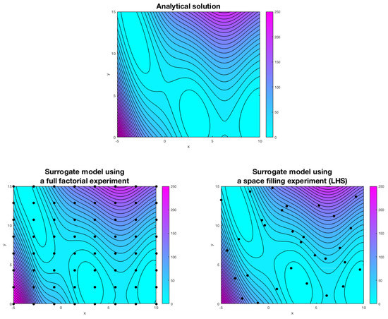
Figure 4.
Top: analytical solution. Bottom-left: surrogate model using a full-factorial experiment with 64 training points. Bottom-right: surrogate model using a space-filling experiment with 30 training points (Latin hypercube sampling, LHS).
The next step consists of generating the surrogate model using the information gathered from the sampling plan. In Figure 4, we show the surrogates for both sampling experiments and the analytical solution. As it can be seen, there is no discernible difference between both models and the analytical solution, and this is an indication that the models are accurate. However, to construct a well-fitted surrogate, the full-factorial experiment needs more observation points (especially in high multi-dimensional cases, where the number of experiments increases to the power of the number of design variables), and this translates into higher computing times. It is clear that the quality of the surrogate depends on the number of observations; therefore, if at this point we observe differences between the meta-model and the analytical solution, we can add new points and compute a better surrogate. In SBO, the model can be trained as we gather the data, and we can even use multi-fidelity models and a mixture of physical experiments and computational experiments to construct the surrogate. Finally, after constructing the meta-model, we can conduct the optimization study at the surrogate level using any optimization method.
To demonstrate the advantages of using SBO, we compared its performance against the performance of a gradient-based method (method of feasible directions [53]), and a derivative-free method (single-objective genetic algorithm or SOGA [54]). All methods used were able to find the three minima; the main difference was the number of iterations used and the information provided by the user to start the optimization algorithm. The gradient-based method used 217 high-fidelity function evaluations, where we used a multi-start technique in which multiple start locations were given (this was needed in order to find the multiple minima), and we computed the gradients using forward differences. The derivative-free method used 1200 high-fidelity iterations and did not require any input information from the user (we used the recommended default parameters). Finally, the SBO method used 30 high-fidelity observations (space-filling experiment). These observations were used to construct the meta-model, then, at the surrogate level, derivative-free and gradient-based methods were used to find the minimum. The SBO method has the added value of showing information about the global design space.
As a final example, let us use the high-dimensional Rosenbrock function to demonstrate the ability of the SBO method in dealing with multivariate problems. The Rosenbrock function can be written in general form as
this equation with the given bounds has one global minimum, defined as follows:
To conduct the SBO study, we proceed in the same way as for the Branin function. At the high-fidelity level, we used two gradient-based methods, namely, the method of feasible directions [53] and the quasi-Newton BFGS update method [55]. Both methods converged to the global minimum, but the BFGS method showed a better convergence rate. At the surrogate level we used three methods: two gradient-based methods (same methods as in the high-fidelity study) and one derivative-free method, namely, the DIRECT method (DIvide a hyperRECTangle [56]). The surrogate was constructed using 500 observations, which roughly correspond to the same number of function evaluations in the best case of the high-fidelity optimization studies (refer to Table 1). It is noteworthy that as we have a mathematical representation of the design space, the gradients were computed analytically during the SBO study.

Table 1.
Outcome of the optimization study of the high-dimensional Rosenbrock function. In the table, observations refer to the number of experiments used to construct the surrogate. Note that the same starting point () was used for all the design variables in the gradient-based optimization studies. In the table, DV stands for design variable, HF stands for high-fidelity simulations, SBO stands for surrogate-based optimization, MFD stands for method of feasible directions, QN stands for quasi-Newton BFGS method, and DR stands for division of rectangles derivative-free method.
The outcome of this SBO study is presented in Table 1. As it can be seen in this table, at the surrogate level, we get values close to the global minimum; but, due to a noisy and under-fitted surrogate, the optimal value is under-predicted. We can also observe that the values of the design variables 4–6 are a little bit over-predicted, but in general they follow the trend of the high-fidelity values. One way to improve the results could be to construct a better surrogate by using a larger number of observations. However, as the number of observations will be much higher than the number of function evaluations in the best case of the high-fidelity optimization studies, the use of SBO is not very attractive, especially if the computation of the QoI is expensive. Another way to improve the surrogate is by using infilling, which consists of adding new points to the training set and then reconstructing the surrogate. For example, we can add a new point in the location of the predicted optimal value and a few new points in areas where high nonlinearities are observed or are close to the optimal value, recompute the surrogate, and find the new optimal value. It is worth mentioning that we also used 200 experiments to conduct the SBO study, but due to the coarseness of the space-filling sampling, the surrogate was under-fitted; therefore, the optimization studies failed to converge or give similar trends to the ones shown in Table 1.
Another advantage of SBO is that we can use exploratory data analysis and machine learning techniques to interrogate the data obtained during the design space exploration stage. These techniques can be used for knowledge extraction and anomaly detection. In Figure 5, we show one of the many plots that can be used to visualize the data [57,58]. This plot is called a scatter matrix, and in one single illustration, it shows the correlation information, the data distribution (using histograms and scatterplots), and regression models of the responses of the QoI. The reader should be aware that, in the context of design space exploration, exploratory data analysis and machine learning methods should not be used with biased data, e.g., data coming from a gradient-based or derivative-free optimization study.
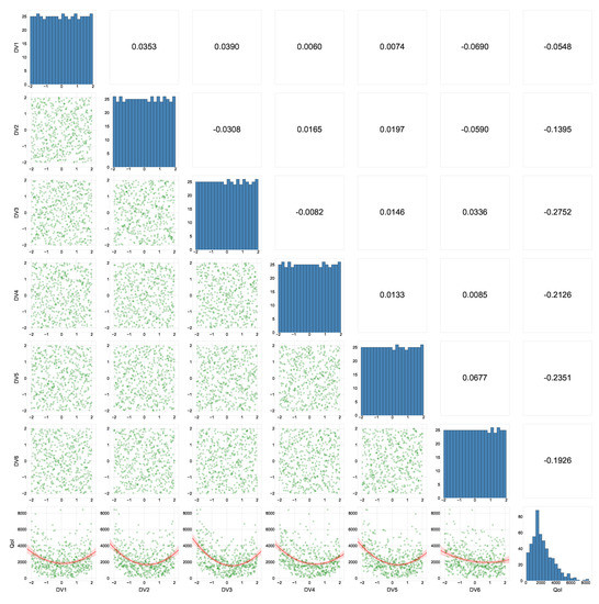
Figure 5.
Scatterplot matrix of the high-dimensional Rosenbrock function space exploration study (). The Spearman correlation is shown in the upper triangular part of the matrix. In the diagonal of the matrix, the histograms showing the data distribution are displayed. In the lower triangular part of the matrix, the data distribution is shown using scatterplots. In the last row of the matrix plot, the response of the quantity of interest (QoI) in function of the design variables is illustrated, together with a quadratic regression model.
By conducting a quick inspection of the scatterplot matrix displayed in Figure 5, we can see evidence that the data is distributed uniformly in the design space (meaning that the sampling plan is unbiased), and this is evidenced by the diagonal of the plot. By looking at the scatterplot of the experiments (lower triangular part of the matrix), we see the distribution of the data in the design space. If at this point we observe regions in the design space that remain unexplored, we can simply add new training points to cover those areas. In the case of outliers (anomalies), we can remove them from the dataset with no major inconvenience. However, we should be aware that outliers are telling us something, so it is a good idea to investigate the cause and effect of the outliers. In the upper triangular part of the plot, the correlation information is shown (Spearman correlation, in this case). This information tells us how correlated or uncorrelated the data are. For example, by looking at the last row of the plot that shows the response of the QoI, if we see a strong correlation between two variables, it is clear that this variable cannot be excluded from the study. The opposite is also true, that is, uncorrelated variables can be excluded from the study; therefore, the complexity of the problem is reduced. One should be aware that for data exclusion using correlation information, we should use the response of the QoI and not the design space distribution of the sampling plan. For a well-designed experiment, the design space distribution is uncorrelated. Additionally, the last row of the scatter matrix plot also shows the regression model (a quadratic model, in this case). As can be seen, this simple plot can be used to gather a deep understanding of the problem.
To close the optimization framework discussion, we would like to stress the fact that the optimization loop implemented is fault tolerant, so in the event of hardware or software failure, the optimization task can be restarted from the last saved state. Moreover, during the optimization loop, all the data monitored are made available immediately to the user, even when running multiple simulations at the same time (real-time data analytics). Therefore, anomalies and trends can be detected in real time, and corrections/decisions can be made.
3. Description of the CFD Model
All the numerical simulations described in this manuscript were conducted using the open-source OpenFOAM library [26,43] (version 5.0). This toolbox is based on the cell-centered finite volume method, and consists of a series of numerical discretization schemes, linear systems solvers, velocity–pressure coupling methods, and physical models that can be used to solve multi-physics problems. To find the approximated numerical solution of the governing equations, and to deal with the physics of segregated multi-phase flows, we used the solver interFoam, which is distributed with OpenFOAM. This solver uses the volume of fluid (VoF) phase-fraction method to resolve the interface between phases and has extensive turbulence modeling capabilities. In this work, we used the SST turbulence model, as described in Reference [59].
3.1. Reference Geometry and Modeling Assumptions
The baseline geometry used in this study was provided by the ship manufacturer Fincantieri and is illustrated in Figure 6. The model is scaled 1/20 in reference to the full-scale prototype, and experimental data from towing tank tests were also provided. Due to the intellectual property of Fincantieri on the prototype and the experimental data, this information cannot be disclosed. Therefore, all the reference values are presented using non-dimensional numbers.
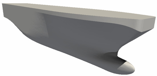
Figure 6.
The baseline geometry.
During the experimental campaign, the following Froude number values were used: 0.294, 0.312, 0.331, 0.349, 0.367, and 0.386. The Froude number is defined as follows:
where V is the velocity, g is the gravity, and L is a reference length. Hereafter, we used the length between perpendiculars or (in naval design, is defined as the distance measured along the load waterline between the after and fore perpendiculars) as the reference length.
The setup of the towing tank tests allowed for the model to dynamically adjust its trim angle (or pitch angle). Conversely, the simulations reported in this manuscript were performed with a fixed trim condition. Even if this simplification can affect the accuracy of the force prediction, it can be considered minor in the context of this optimization study. This is chiefly due to the fact that the bulb shape modifications can be assumed to be uninfluential to the final dynamic trim. Furthermore, low trim angle values are recorded in the experimental data. These values are less than two degrees for the most critical case, that is, high Froude number (or off-design conditions). In addition, the use of a rigid-body motion solver would have considerably increased the computational requirements and CPU time.
Hereafter, we summarize the main assumptions used during this study:
- All simulations were performed at model scale (1/20).
- No propeller nor appendages were modeled (bare hull).
- Only half of the hull was simulated (we used symmetry).
- A fixed trim condition of zero degrees was imposed.
- All the simulations were conducted in calm water conditions and no incoming waves.
- The thermophysical properties of the working fluids are constant (refer to Table 2).
Table 2. Phases transport properties used in this study.
- The simulations were conducted at the same Froude number as in the towing tank experiments.
As we are conducting a bulbous bow optimization study, we must define the design variables. In this study, we used the parameters proposed by Kracht [20]. Kracht defined six parameters to characterize a bulbous bow, namely, length, depth, and breadth (all linear); the cross-section; and lateral and volumetric parameters (which are nonlinear). Hereafter, the bulb geometry was parameterized using the length parameter (or protrusion) and depth parameter (or immersion). These parameters are defined as follows (as illustrated in Figure 7):
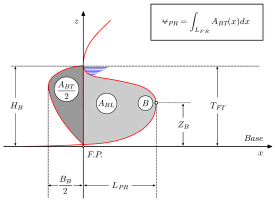
Figure 7.
Sketch showing the characteristic lengths used to define the geometry parameters. Adapted from Reference [20].
These two parameters were enough to deform the geometry, and as we only used two design variables, the design space was greatly simplified. The choice of these two parameters (in reference to Figure 7), was driven by the interest of only moving point B in the plane x-z, as recommended by Fincantieri. This together with the suggested bounds ( and ) will ensure that the bulbous bow volume variations remain within the acceptable values, without the need for introducing additional design variables and nonlinear constraints.
3.2. Computational Domain and Boundary Conditions
The computational domain is aligned with the reference system and is made up of a rectangular box in which half of the hull geometry was placed (as depicted in Figure 8). In the domain, the x-max face represents the inlet (where air and water enter the domain at a given velocity), the x-min face is the outlet (where air and water go out of the domain and the water level is maintained at the same level of the inlet level), the y-max face is the symmetry plane, the y-min face is a lateral slip wall, the z-min face is the bottom of the domain modeled as a slip wall, and the z-max face is the top of the domain, which is defined as an opening where only the air phase is allowed to enter or exit the domain. The inlet and outlet patches are located and away from the bow and stern. The top and bottom faces are placed at and away from the sea level. The lateral face is placed at away from the symmetry plane to avoid lateral reflection of the Kelvin waves. In general, the boundaries were placed far enough of the hull surface so there are no significant gradients normal to the boundaries or wave reflection. When setting the domain, we followed the practical guidelines given in Reference [60].
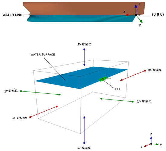
Figure 8.
Top: coordinate system. Bottom: computational domain and boundary faces.
The hull was modeled as a no-slip wall, where we imposed wall function boundary conditions for the turbulence variables. The forces on the hull were computed by integrating the viscous and pressure forces over the hull surface. Finally, all the simulations were started using uniform initial conditions for both phases. In the domain, the water phase is located below the origin of the coordinates system, whereas the air phase is located above the coordinate system origin. All the turbulence variables were initialized following the guidelines given by Wilcox [59].
3.3. Numerical Schemes
Hereafter, we describe the numerical setup used with OpenFOAM. During this study, a robust, stable, and high-resolution numerical scheme was used. The cell-centered values of the variables are interpolated at the face locations using a second-order centered differences scheme for the diffusive terms. The convective terms are discretized by means of a second-order linear-upwind scheme, and to prevent spurious oscillations, a multi-dimensional slope limiter was used. To resolve the interface between the two phases, the second-order accurate bounded total variation diminishing (TVD) scheme of van Leer was used. For computing the gradients at the cell centers, the least squares cell-based reconstruction method was employed. The pressure–velocity coupling was achieved by means of the pressure-based PISO method. For turbulence modeling, the SST turbulence model with wall functions was used [59].
As stated earlier, one of the biggest restrictions when conducting optimization studies in CFD is the long simulation times, especially if unsteady simulations are involved. To overcome this hurdle, we aimed at accelerating the solution of the governing equations by looking for steady-state solutions. In this study, we used the local time-stepping (LTS) method. In this method, the governing equations are integrated in time using the largest possible time step for each cell. As a result, the convergence to the steady state is considerably accelerated; however, the transient solution is no longer time accurate. The stability and accuracy of the method are driven by the local CFL number of each cell, which was fixed to 0.1 during the initial iterations and then gradually increased until reaching a value of 0.9. To avoid further instabilities due to large conservation errors caused by sudden changes in the time-step of each cell, the local time-step was smoothed and damped across the domain.
4. Calibration and Validation of the Solver
The purpose of this section is twofold. First, we validate the solver against the experimental data available, and secondly, we calibrate the parameters of the solver and the mesher. In other words, we look for the best parameters to be used during the optimization study, and in the case of meshing or convergence problems, these parameters are automatically adjusted without user intervention.
In Table 3, we list the cell count and average of the coarse and fine mesh used in this study. We used at least five inflation layers to resolve the boundary layer, and we targeted for a value between 40 and 200. The results obtained from transient simulations and steady simulations using the LTS method are displayed in Figure 9. The results illustrated correspond to the base geometry and a Froude number equal to 0.331. Due to the intellectual property of the experimental data, from this point on, all the results are normalized using as a reference the experimental value corresponding to this operating condition.
Table 3.
Mesh cell count and average .
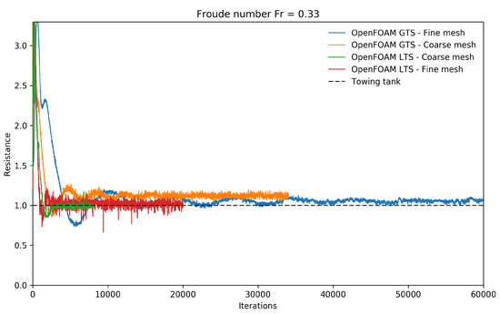
Figure 9.
Comparison of the normalized resistance as a function of the iteration number for the coarse and fine meshes. In the legend, LTS (local time-stepping) corresponds to the steady solution, and GTS (global time-stepping, i.e., a time-step identical for all control volumes) corresponds to the transient solutions.
In Figure 9, we can observe that the outcome of the steady simulations using both meshes are in good agreement with the experimental values. Both solutions reached a steady state approximately after 4000 iterations. Nevertheless, we let the simulations run for longer times to ascertain that we reached good iterative convergence. Regarding the unsteady simulations, we can see that the simulation using the fine mesh reached periodic iterative convergence after approximately 40,000 iterations. On the other hand, the unsteady simulation using the coarse mesh reached a periodic iterative convergence after about 20,000 iterations. However, the results are slightly over-predicted due to numerical diffusion and turbulence model uncertainties. For the unsteady simulations, the time-step was chosen in such a way that the maximum CFL number is equal to 2, whereas, for the steady simulations (where we used the LTS method), the CFL number was gradually increased until reaching the value of 0.9.
In Table 4, we show the percentage error (computed with respect to the experimental data) and the CPU time measured at 8000 iterations for each simulation plotted in Figure 9. From these results, it becomes clear why it is important to find steady solutions when conducting optimization studies in CFD. If we had conducted this optimization study using an unsteady solver, the computing time of each simulation would have been about 2 times the computing time of the corresponding steady simulation (for the same number of iterations); therefore, the total computing time of the optimization loop would have been at least 2 times higher.
Table 4.
Percentage error (with respect to the experimental data) and CPU time of the benchmark cases. All the simulations were run in parallel with four processors. In all cases, the reported CPU time was measured at 8000 iterations.
In Figure 10, we present the normalized resistance as a function of the Froude number. The results reported were obtained using the coarse mesh and the LTS method. In the figure, a good agreement with the experimental results is observed up to a value of , then, the percentage error starts to increase, and this is mainly due to the fixed trim condition assumption used in this study. Moreover, the prototype is not meant to operate at such high Froude numbers, which corresponds to off-design conditions. In the light of this optimization study, where we know there are many uncertainties involved, errors of this order of magnitude are acceptable given the assumptions that were taken. Also, these discrepancies can be neglected because it is reasonable to consider that this error is constant for each bulb shape to be simulated and is, therefore, irrelevant for the optimization loop.
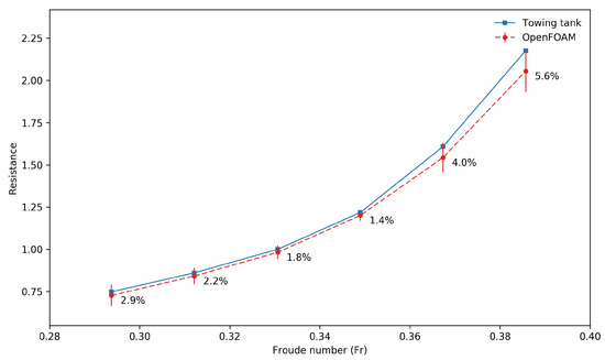
Figure 10.
Comparison of the normalized resistance as a function of the Froude number. The numbers next to the markers indicate the percentage error between the numerical results and the experimental data.
Based on these results, we decided to use the coarse mesh as the base mesh, and in the case of mesh quality problems, the domain mesh was automatically recomputed using improved meshing parameters. As for the iterative method concerns, all the simulations were executed using the LTS method, and if proper iterative convergence was reached, the simulations were automatically stopped at 8000 iterations or until statistically stable results were obtained. These choices allowed us to obtain fast outcomes with good accuracy.
5. Results and Discussion
Hereafter, we discuss the results obtained from the surrogate-based optimization study. All the simulations presented in this section were conducted at a Froude number of 0.294. We would like to stress that to get the optimization loop started, we only need one input geometry. Then, this geometry is deformed by the shape morpher to generate new candidates. Also, the whole optimization framework was deployed using asynchronous simulations: that is, we executed many parallel simulations at the same time. Everything was controlled using the application coupling interface provided by Dakota. The average time of each simulation was between 4 and 5 hours.
As discussed previously, the first step when conducting SBO studies is to generate a sampling plan of the design space. The sampling plan should cover the design space in a uniform and well-distributed way, without leaving large areas unexplored; also, it should be cheap to compute. It is clear that the more information we gather during the initial sampling, the better the surrogate will be, but at the cost of longer computing times. In this study, we used a full-factorial experiment, where we conducted 25 experiments uniformly spaced in the design space. In Figure 11, we illustrate the sampling plan, where the uniform spaced points represent the locations where the high-fidelity computations were computed. The sampling plan illustrated in Figure 11 was chosen because it is inexpensive to compute (as we reduced the number of design variables to two), and it explores design points without missing too much information between observations.
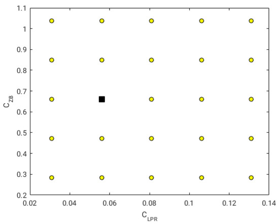
Figure 11.
Sampling plan used in this study. The square represents the original geometry, whereas the circles represent the different geometry variations. Every point in the sampling plan represents a location where a high-fidelity computation was computed. All the simulations were conducted at a Froude number of 0.294.
The next step in our work-flow is to construct the surrogate (or meta-model) after conducting the high-fidelity simulations at the sampling locations. In this study, we used Kriging interpolation [38,44,45,48,49,50,51,52], which has been demonstrated to be a very reliable and accurate interpolation method when conducting SBO studies. The only drawback of this method (if it can be considered a drawback) is that it forces the meta-model to pass by all the points of the sampling plan; therefore, in the presence of numerical noise, we can have surrogates with many valleys and peaks that can make the optimization task difficult when using gradient-based methods. Nevertheless, as we are working at the surrogate level, we can use derivative-free methods which behave better in the presence of numerical noise.
In Figure 12, we illustrate two surrogates obtained during this study. In the figure, the surrogate in the left image was constructed using Kriging interpolation, and the one in the right image was build using a second-order polynomial function. The color scale represents the resistance variation in reference to the original geometry (where negative values indicate resistance reduction and positive values indicate resistance increment). As it can be seen, the Kriging model managed to capture the nonlinearities of the design space; we can even distinguish a valley region where the optimal solution (or solutions) might be located. On the other hand, the polynomial model is very smooth; however, it is not very accurate (it does not capture the nonlinearities). Nevertheless, it gives us a rough idea of how the design space behaves.
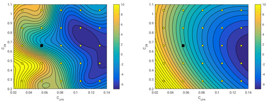
Figure 12.
Left: surrogate model constructed using Kriging interpolation. Right: surrogate model constructed using quadratic polynomial interpolation. In the image, the uniform spaced points represent the locations where the high-fidelity computations were computed. The square represents the starting geometry and the circles represent the new geometries. In both images, the color scale represents the resistance variation in reference to the original geometry (where negative values indicate resistance reduction, and positive values indicate resistance increment).
At this stage, we already have a surrogate of the design space, or in other words, a mathematical representation of the design space. Our next tasks consist of validating the surrogate and conducting the optimization study at the surrogate level. The validation merely consists of computing the predicted value at the surrogate level in a location that has not been included in the sampling plan. Then, this value can be compared with the value obtained using high-fidelity simulations in the same location, and the percentage error can be computed. The optimization consists of doing the actual optimization at the surrogate level. Remember, as we are working using a mathematical representation of the design space, we can use any optimization method, disregarding how expensive it can be.
In this study, we found a global minimum and a local minimum; this situation is illustrated in Figure 13. These results suggest that there is a bifurcation in the valley region, where the global minimum is obtained when increasing the value of the design variable , and the local minimum is obtained when decreasing the value of the design variable . Notice also that as we increase the value of the design variable , smaller increments of the design variable are required in order to obtain larger resistance reduction. In Figure 13 (right image), we show the iterative path followed by the optimization algorithm when starting from two different initial positions, where each optimization task used about 40 iterations (function evaluations and gradient evaluations). As we used a gradient-based method to optimize the surrogate (method of feasible directions [53]), it is clear that we need to start the optimization algorithm from different initial locations if we want to find the global and local minima. If we were to perform this study by directly resorting to high-fidelity simulations, the number of simulations would be much higher than the number of simulations used during the sampling plan.
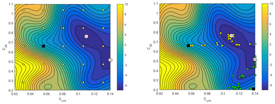
Figure 13.
Left: the × symbol represents the global minimum, and the + symbol represents the local minimum. The square represents the starting geometry and the circles represent the new geometries. Right: the two squares represent two different starting points of the optimization algorithm. The yellow circles represent the path followed by the gradient-based algorithm when starting from the topmost position, whereas the green circles represent the path followed by the gradient-based algorithm when starting from the bottom-most position. In both images, the color scale represents the resistance variation in reference to the original geometry (where negative values indicate resistance reduction, and positive values indicate resistance increment).
As previously mentioned, the SBO method gives the possibility of conducting an initial screening (or visualization) of the design space. This initial screening can be extremely helpful, especially when dealing with high multi-dimensional optimization problems. By screening the surrogate, designers can explore and exploit the surrogate in a more efficient way. Different optimal candidates can be immediately identified through the subjective opinion of the designer or on the basis of external constraints (such as manufacturing process, increased weight due to the added surface, the volume of the new bulb, structural loads, clearances, and so on), without the need of resorting to high-fidelity simulations (with the exception of the validation of the surrogate).
To demonstrate the validity of the surrogate, in Table 5, we show the numerical values of the resistance reduction and the percentage error between the surrogate value and the high-fidelity simulations outcome. The values presented in this table were measured in five different points; namely, the global minimum, the local minimum, and three points in the proximity of the global and local minima. From the table, we observe that all values listed effectively reduce the resistance. We also observe that the percentage error between the surrogate level and the high-fidelity level is about 2% for the global and local minima cases. On the other hand, for the values measured in the vicinity of the global and local minima, the percentage error is much larger, and this is presumably because in this region the nonlinearities are more significant.
Table 5.
Resistance reduction and percentage error (with respect to the high-fidelity simulations) of five cases not included in the original sampling plan.
We can also improve the surrogate by adding new points to it (this is known as infilling). For example, we can add the points listed in Table 5 ( and ) and recompute a new surrogate (and optimal values). This situation is illustrated in Figure 14, where the triangle symbols represent the new training points. In the surrogate pictured in the figure, we are able to capture with more details the behavior of the design space close to the region where the global minimum is located. Also, we still can see the bifurcation, where there is a clear optimal solution when we increase the value of ; however, when decreasing the value , the location of the new minimum is not very clear. It may be necessary to add a new training point in this region in order to get a better surrogate. Nevertheless, the resistance reduction values in this region are smaller; therefore, we can focus our attention on the cases where we increase the value of .
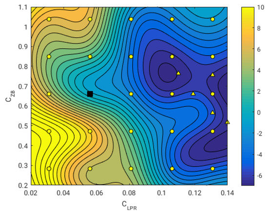
Figure 14.
Improved surrogate using infilling. The square represents the starting geometry and the circles represent the new geometries. The triangles represent the infill points used. The color scale represents the resistance variation in reference to the original geometry (where negative values indicate resistance reduction, and positive values indicate resistance increment).
For completeness, in Figure 15, we show the shape of the optimal bulbs at the design conditions corresponding to the global minimum and the local minimum. From all the results presented in this section, it is clear that surrogate-based optimization is an effective design tool for engineering design. However, the user should be cautious when constructing the surrogate, because the whole method depends on the quality of the meta-model. It is always recommended to validate the surrogate, do infilling using the optimal solutions, and add a couple of extra points in areas where high nonlinearities are observed or are close to the optimal values.
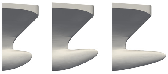
Figure 15.
Bulbous bow shapes. Left: original shape. Middle: shape obtained at global minimum. Right: shape obtained at local minimum.
6. Conclusions and Future Perspectives
In this manuscript, we present an open-source optimization framework to perform industrial optimization studies. The optimization loop implemented allows for asynchronous simulations (i.e., many simulations can be run at the same time), and each simulation can be run in parallel; this allows to considerably reduce the output time of the optimization iterations. The optimization loop is fault tolerant and software agnostic, and it can be interfaced with any application able to interact using input/output files via a command line interface. The code coupling capabilities were provided by the library Dakota [28], and all the tools used in this work are open-source and free.
As for the optimization strategy concerns, we used surrogate-based optimization; this technique is very well suited to engineering design, as it allows designers and engineers to efficiently optimize and explore the design space from a limited number of training observations, without resorting to too many expensive high-fidelity simulations. To demonstrate the usability and flexibility of the proposed framework, we tested it in a practical case related to the naval industry, where we aimed at optimizing the shape of a bulbous bow to minimize the hydrodynamic resistance. We must highlight that the framework discussed in this work is general enough so that it may be used in any engineering design application.
During the optimization at the surrogate level, we found a global minimum. The shape of the optimal solution at the global minimum corresponds to a longer bulb and slightly shifted upwards. The resistance reduction at the global minimum design conditions is on the order of at the surrogate level. The difference in resistance reduction between the global minimum at the surrogate level and the corresponding high-fidelity value is on the order of (which is deemed more than acceptable). However, as optimization can be very abstract (e.g., balance between aesthetics and usability, operational requirements related to clearances, constraints related to weather conditions, ease of manufacturing new shapes, and so on), we further explored the meta-model and we found a local minimum corresponding to a configuration where we decreased the value of the design variable in reference to the original geometry. At this design condition, the resistance reduction is on the order of , with a difference between the local minimum at the surrogate level, and the corresponding high-fidelity value on the order of . At this point, the optimal solution depends on the designer criteria and external constraints. These results demonstrate that design candidates showing considerable resistance reduction can be found using surrogate-based optimization, with very affordable computational times for the overall optimization task.
Finally, the results presented are limited to fixed trim, two design variables of the bulbous bow, and a single Froude number for the optimization study. We envisage the extension of the current work to rigid body simulations, and the exploration of the design space at different Froude numbers to determine if there is a dependence between protrusion and immersion of the bulbous bow and Froude number. We also look upon using a more complex parameterization of the bulbous bow geometry and conducting multi-objective optimization.
Author Contributions
Conceptualization, A.C., D.V., J.G. and J.P.; Methodology, A.C. and J.G.; Software, A.C. and J.G.; Validation, A.C. and J.G.; Formal Analysis, A.C.; Investigation, A.C., D.V., J.G. and J.P.; Resources, J.G.; Data Curation, A.C. and J.G.; Writing—Original Draft Preparation, A.C. and J.G.; Writing—Review & Editing, D.V., J.G. and J.P.; Visualization, A.C. and J.G.; Supervision, J.P.
Acknowledgments
We thank Fincantieri for making the solid model and experimental data available and for the support provided. We also thanks the DTLM (http://www.dltm.it), for letting us use their HPC facilities and the support provided.
Conflicts of Interest
The authors declare no conflict of interest.
References
- Gaggero, S.; Tani, G.; Villa, D.; Viviani, M.; Ausonio, P.; Travi, P.; Bizzarri, G.; Serra, F. Efficient and multi-objective cavitating propeller optimization: An application to a high-speed craft. Appl. Ocean Res. 2017, 64, 31–57. [Google Scholar] [CrossRef]
- Vesting, F.; Bensow, R.E. On surrogate methods in propeller optimization. Ocean Eng. 2014, 88, 214–227. [Google Scholar] [CrossRef]
- Paik, B.G.; Kim, G.D.; Kim, K.Y.; Seol, H.S.; Hyun, B.S.; Lee, S.G.; Jung, Y.R. Investigation on the performance characteristics of the flexible propellers. Ocean Eng. 2013, 73, 139–148. [Google Scholar] [CrossRef]
- Gaggero, S.; Gonzalez-Adalid, J.; Sobrino, M. Design and analysis of a new generation of CLT propellers. Appl. Ocean Res. 2016, 59, 424–450. [Google Scholar] [CrossRef]
- Vernengo, G.; Bonfiglio, L.; Gaggero, S.; Brizzolara, S. Physics-Based Design by Optimization of Unconventional Supercavitating Hydrofoils. J. Ship Res. 2016, 60, 187–202. [Google Scholar] [CrossRef]
- Harries, S. Parametric Design and Hydrodynamic Optimization of Ship Hull Forms; Mensch-und-Buch-Verlag: Berlin, Germany, 1998. [Google Scholar]
- Campana, E.; Peri, D.; Tahara, Y.; Stern, F. Shape optimization in ship hydrodynamics using computational fluid dynamics. Comput. Methods Appl. Mech. Eng. 2006, 196, 634–651. [Google Scholar] [CrossRef]
- Tahara, Y.; Peri, D.; Campana, E.; Stern, F. Computational fluid dynamics-based multi-objective optimization of a surface combatant using a global optimization method. J. Mar. Sci. Technol. 2008, 13, 95–116. [Google Scholar] [CrossRef]
- Biliotti, I.; Brizzolara, S.; Viviani, M.; Vernengo, G.; Ruscelli, D.; Galliussi, M.; Guadalupi, D.; Manfredini, A. Automatic parametric hull form optimization of fast naval vessels. In Proceedings of the 11th International Conference on Fast Sea Transportation, Honolulu, HI, USA, 26–29 September 2011. [Google Scholar]
- Vernengo, G.; Brizzolara, S.; Bruzzone, D. Resistance and sea-keeping optimization of a fast multi-hull passenger ferry. Int. J. Offshore Polar Eng. 2015, 25, 26–34. [Google Scholar]
- Tahara, Y.; Peri, D.; Campana, E.; Stern, F. Single- and multi-objective design optimization of a fast multi-hull ship: Numerical and experimental results. J. Mar. Sci. Technol. 2011, 16, 412–433. [Google Scholar] [CrossRef]
- Vernengo, G.; Brizzolara, S. Numerical investigation on the hydrodynamic performance of fast SWATHs with optimum canted struts arrangements. Appl. Ocean Res. 2017, 63, 76–89. [Google Scholar] [CrossRef]
- Serani, A.; Leotardi, C.; Iemma, U.; Campana, E.; Fasano, G.; Diez, M. Parameter selection in synchronous and asynchronous deterministic particle swarm optimization for ship hydrodynamics problems. Appl. Soft Comput. 2016, 49, 313–334. [Google Scholar] [CrossRef]
- Chen, X.; Diez, M.; Kandasamy, M.; Zhang, Z.; Campana, E.; Stern, F. High-fidelity global optimization of shape design by dimensionality reduction, meta-models and deterministic particle swarm. Eng. Optim. 2015, 47, 473–494. [Google Scholar] [CrossRef]
- Peri, D.; Tinti, F. A multi-start gradient-based algorithm with surrogate model for global optimization. Commun. Appl. Ind. Math. 2012, 3, 1–22. [Google Scholar]
- Demo, N.; Tezzele, M.; Gustin, G.; Lavini, G.; Rozza, G. Shape optimization by means of proper orthogonal decomposition and dynamic mode decomposition. In Proceedings of the NAV 2018, Trieste, Italy, 20–22 June 2018; pp. 212–219. [Google Scholar]
- Umetani, N.; Bickel, B. Learning Three-dimensional Flow for Interactive Aerodynamic Design. ACM Trans. Graph. 2018, 37. [Google Scholar] [CrossRef]
- Li, J.; Bouhlel, M.A.; Martins, J.R.R.A. A data-based approach for fast airfoil analysis and optimization. In Proceedings of the 2018 AIAA/ASCE/AHS/ASC Structures, Structural Dynamics, and Materials Conference, Kissimmee, FL, USA, 8–12 January 2018. [Google Scholar]
- Matejka, J.; Glueck, M.; Bradner, E.; Hashemi, A.; Grossman, T.; Fitzmaurice, G. Dream Lens: Exploration and Visualization of Large-Scale Generative Design Datasets. In Proceedings of the ACM CHI Conference on Human Factors in Computing Systems, Montreal, QC, Canada, 21–26 April 2018. [Google Scholar]
- Kracht, A.M. Design of bulbous bow. SNAME Trans. 1978, 86, 197–217. [Google Scholar]
- Huang, F.; Yang, C. Hull form optimization of a cargo ship for reduced drag. J. Hydrodyn. Ser. B 2016, 28, 173–183. [Google Scholar] [CrossRef]
- Lu, Y.; Chang, X.; Hu, A. A hydrodynamic optimization design methodology for a ship bulbous bow under multiple operating conditions. Eng. Appl. Comput. Fluid Mech. 2016, 10, 330–345. [Google Scholar] [CrossRef]
- Mahmood, S.; Huang, D. Computational fluid dynamics based bulbous bow optimization using a genetic algorithm. J. Mar. Sci. Appl. 2012, 11, 286–294. [Google Scholar] [CrossRef]
- Luo, W.; Lan, L. Design Optimization of the Lines of the Bulbous Bow of a Hull Based on Parametric Modeling and Computational Fluid Dynamics Calculation. Math. Comput. Appl. 2017, 22, 4. [Google Scholar] [CrossRef]
- Bolbot, V.; Papanikolaou, A. Parametric, multi-objective optimization of ship’s bow for the added resistance in waves. Ship Technol. Res. 2016, 63, 171–180. [Google Scholar] [CrossRef]
- OpenFOAM Web Page. Available online: http://openfoam.com (accessed on 12 October 2018).
- Mimmo Web Page. Available online: http://optimad.github.io/mimmo (accessed on 12 October 2018).
- Dakota Web Page. Available online: https://dakota.sandia.gov/ (accessed on 12 October 2018).
- Spisso, I. Parametric and Optimization Study: OpenFOAM and Dakota. In Proceedings of the Workshop on HPC Enabling of OpenFOAM for CFD Applications, Bologna, Italy, 26–28 November 2012. [Google Scholar]
- Geremia, P. Industrial design optimization using open source tools. In Proceedings of the 6th OpenFOAM® Workshop, University Park, PA, USA, 13–16 June 2011. [Google Scholar]
- Geremia, P.; de Villiers, E. Open source software tools for powertrain optimization. In Proceedings of the 6th OpenFOAM® Workshop, University Park, PA, USA, 13–16 June 2011. [Google Scholar]
- Skuric, V.; Uroic, T.; Rusche, H. Multi-objective optimization of a tube bundle heat exchanger. In Proceedings of the 9th OpenFOAM® Workshop, Zagreb, Croatia, 23–26 June 2014. [Google Scholar]
- Byrne, J.; Cardiff, P.; Brabazon, A.; O’Neill, M. Evolving parametric aircraft models for design exploration. J. Neurocomput. 2014, 142, 39–47. [Google Scholar] [CrossRef]
- Ohm, A.; Tetursson, H. Automated CFD Optimization of a Small Hydro Turbine for Water Distribution Networks; Chalmers University of Technology: Göteborg, Sweden, 2017. [Google Scholar]
- Oh, J.T.; Chien, N.B. Optimization design by coupling computational fluid dynamics and genetic algorithm. In Computational Fluid Dynamics; IntechOpen: London, UK, 2018. [Google Scholar]
- Lee, W.H.; Oh, S.H.; Lee, S.D. Deciding optimal parameter for internal wavemaker using coupling of Dakota and OpenFOAM. In Proceedings of the 13th OpenFOAM® Workshop, Shanghai, China, 24–29 June 2018. [Google Scholar]
- Slotnick, J.; Khodadoust, A.; Alonso, J.; Darmofal, D.; Gropp, W.; Lurie, E.; Mavriplis, D. CFD Vision 2030 Study: A Path To Revolutionary Computational Aerosciences; NASA: Hampton, VA, USA, 2014.
- Adams, B.M.; Ebeida, M.S.; Eldred, M.S.; Geraci, G.; Jakeman, J.D.; Maupin, K.A.; Monschke, J.A.; Swiler, L.P.; Stephens, J.A.; Vigil, D.M.; et al. Dakota, A Multilevel Parallel Object-Oriented Framework for Design Optimization, Parameter Estimation, Uncertainty Quantification, and Sensitivity Analysis: Version 6.5 User Manual; Sandia National Laboratories: Albuquerque, NM, USA, 2014.
- Scardigli, A.; Arpa, R.; Chiarini, A.; Telib, H. Enabling of Large Scale Aerodynamic Shape Optimization through POD-Based Reduced-Order Modeling and Free Form Deformation. In Proceedings of the EUROGEN 2015, Glasgow, UK, 14–16 September 2015. [Google Scholar]
- Crane, K.; Weischedel, C.; Wardetzky, M. Geodesics in Heat: A New Approach to Computing Distance Based on Heat Flow. ACM Trans. Graph. 2013, 32, 1–11. [Google Scholar] [CrossRef]
- Buhmann, M.D. Radial Basis Function: Theory and Implementations; Cambrige University Press: Cambrige, UK, 2003. [Google Scholar]
- Salmoiraghi, F.; Scardigli, A.; Telib, H.; Rozza, G. Free-form deformation, mesh morphing and reduced-order methods: enablers for efficient aerodynamic shape optimisation. Int. J. Comput. Fluid Dyn. 2018. [Google Scholar] [CrossRef]
- Weller, H.G.; Tabor, G.; Jasak, H.; Fureby, C. A tensorial approach to computational continuum mechanics using object-oriented techniques. Comput. Phys. 1998, 12, 620–631. [Google Scholar] [CrossRef]
- Forrester, A.; Sobester, A.; Keane, A. Engineering Design via Surrogate Modeling. A Practical Guide; Wiley: New York, NY, USA, 2008. [Google Scholar]
- Dalbey, K.R. Efficient and Robust Gradient Enhanced Kriging Emulators; Sandia National Laboratories: Albuquerque, NM, USA, 2013.
- Jones, D.R.; Schonlau, M.; Welch, W.J. Efficient global optimization of expensive black-box functions. J. Glob. Optim. 1998, 13, 455–492. [Google Scholar] [CrossRef]
- Iuliano, E.; Perez, E.A. Application of Surrogate-Based Global Optimization to Aerodynamic Design; Springer: Basel, Switzerland, 2016. [Google Scholar]
- Oliver, M.; Webster, R. Kriging: A Method of Interpolation for Geographical Information Systems. Int. J. Geogr. Inf. Syst. 1990, 4, 313–332. [Google Scholar] [CrossRef]
- Adams, B.M.; Ebeida, M.S.; Eldred, M.S.; Geraci, G.; Jakeman, J.D.; Maupin, K.A.; Monschke, J.A.; Swiler, L.P.; Stephens, J.A.; Vigil, D.M.; et al. Dakota, A Multilevel Parallel Object-Oriented Framework for Design Optimization, Parameter Estimation, Uncertainty Quantification, and Sensitivity Analysis: Version 6.5 Theory Manual; Sandia National Laboratories: Albuquerque, NM, USA, 2014.
- Dalbey, K.R.; Giunta, A.A.; Richards, M.D.; Cyr, E.C.; Swiler, L.P.; Brown, S.L.; Eldred, M.S.; Adams, B.M. Surfpack User’s Manual Version 1.1; Sandia National Laboratories: Albuquerque, NM, USA, 2013.
- Giunta, A.A.; Watson, L. A comparison of approximation modeling techniques: polynomial versus interpolating models. In Proceedings of the 7th AIAA/USAF/NASA/ISSMO Symposium on Multidisciplinary Analysis and Optimization, St. Louis, MO, USA, 2–4 September 1998. [Google Scholar]
- Romero, V.J.; Sqiler, L.P.; Giunta, A.A. Construction of response surfaces based on progressive lattice-sampling experimental designs. Struct. Saf. 2004, 26, 201–219. [Google Scholar] [CrossRef]
- Zoutendijk, G. Methods of Feasible Directions: A Study in Linear and Non-Linear Programming; Elsevier: Amsterdam, The Netherlands, 1960. [Google Scholar]
- Gen, M.; Cheng, R. Genetic Algorithms and Engineering Optimization; Wiley-Interscience: New York, NY, USA, 2000. [Google Scholar]
- Vassiliadis, V.S.; Conejeros, R. Broyden family methods and the BFGS update. In Encyclopedia of Optimization; Floudas, C.A., Pardalos, P.M., Eds.; Springer: Boston, MA, USA, 2008. [Google Scholar]
- Jones, D.R.; Perttunen, C.D.; Stuckman, B.E. Lipschitzian optimization without the Lipschitz constant. J. Optim. Theory Appl. 1993, 79, 157–181. [Google Scholar] [CrossRef]
- Guerrero, J.; Bailardi, G.; Kifle, H. Visual storytelling and data visualization in numerical simulations. In Proceedings of the 11th OpenFOAM® Workshop, Guimarães, Portugal, 26–30 June 2016. [Google Scholar]
- Guerrero, J. Opportunities and Challenges in CFD Optimization: Open Source Technology and the Cloud. In Proceedings of the Sixth Symposium on OpenFOAM® in Wind Energy, Gotland, Sweden, 13–14 June 2018. [Google Scholar]
- Wilcox, D.C. Turbulence Modeling for CFD; DCW Industries: La Cañada Flintridge, CA, USA, 2010. [Google Scholar]
- Practical Guidelines for Ship Resistance CFD. Available online: https://ittc.info/media/4198/75-03-02-04.pdf (accessed on 12 October 2018).


© 2018 by the authors. Licensee MDPI, Basel, Switzerland. This article is an open access article distributed under the terms and conditions of the Creative Commons Attribution (CC BY) license (http://creativecommons.org/licenses/by/4.0/).