A (p,q)-Averaged Hausdorff Distance for Arbitrary Measurable Sets

Abstract

The Hausdorff distance is a widely used tool to measure the distance between different sets. For the approximation of certain objects via stochastic search algorithms this distance is, however, of limited use as it punishes single outliers. As a remedy in the context of evolutionary multi-objective optimization (EMO), the averaged Hausdorff distance ${\Delta }_p$ has been proposed that is better suited as an indicator for the performance assessment of EMO algorithms since such methods tend to generate outliers. Later on, the two-parameter indicator ${\Delta }_{p,q}$ has been proposed for finite sets as an extension to ${\Delta }_p$ which also averages distances, but which yields some desired metric properties. In this paper, we extend ${\Delta }_{p,q}$ to a continuous function between general bounded subsets of finite measure inside a metric measure space. In particular, this extension applies to bounded subsets of ${\mathbb{R}}^k$ endowed with the Euclidean metric, which is the natural context for EMO applications. We show that our extension preserves the nice metric properties of the finite case, and finally provide some useful numerical examples that arise in EMO.

1. Introduction

The Hausdorff distance $d_H$ (see [1]) is an established and widely used tool to measure the proximity of different sets. It is, among others, used in several research fields such as image matching (e.g., [2,3,4]), the approximation of manifolds in dynamical systems ([5,6,7]), in fractal geometry ([8]), or in the context of convergence analysis in multi-objective optimization ([9,10,11,12,13]). One major reason for the use of $d_H$ is that it defines a metric on the set of all nonempty bounded closed sets in a metric space. However, one characteristic of the Hausdorff distance is that it heavily punishes single outliers which is a severe drawback in many cases. For instance, it is known that stochastic search algorithms are generally quite effective in the (global) approximation of certain objects, however, it is also known that these approximations may come with a few outliers (e.g., [14]). For those cases, the approximation quality is not reflected by the value of the Hausdorff distance.

As a remedy, in the context of evolutionary multi-objective optimization, Schütze et al. [14] have made a first effort to propose the averaged Hausdorff distance ${\Delta }_p$. As opposed to $d_H$, this indicator averages the distances involved in the proximity measure of the given sets and is hence much more suitable in the context of stochastic search as single (or few) outliers in a candidate solution set are not punished hard any more. On the other hand, compared to $d_H$, ${\Delta }_p$ has two shortcomings: (i) it only defines an inframetric instead of a metric; and (ii) it is only defined for finite approximations of the solution set. In the particular context of continuous multi-objective optimization, it is known that the solution set, the so-called Pareto set, and its image, the Pareto front, form manifolds of certain dimensions. Hence, it is natural that the candidate solution set (i.e., the set computed by a given solver) is not restricted to finitely many points, but may also form a continuous set. This is in fact already the case for set-based optimization techniques such as the cell-to-cell mappings ([15,16,17]) and the subdivision techniques ([10,18,19]). In the context of evolutionary multi-objective optimization, typically a finite set of candidate solutions (a population) is generated ([20,21,22,23]). However, also here it is a rather natural approach to construct a continuous set out of the final population using, e.g., interpolation techniques (see [24,25]).

In [26], a modification of the ${\Delta }_p$ indicator called the $(p,q)$-averaged Hausdorff distance ${\Delta }_{p,q}$ has been introduced by the first two authors. This indicator generalizes the averaged Hausdorff distance ${\Delta }_p$, is strongly related to the Hausdorff distance $d_H$, and admits an expression in terms of the matrix ${\ell }_{p,q}$-norm ${\parallel ·\parallel }_{p,q}$. Moreover, when $1⩽p,q<\infty$ it is a proper metric, while for the remaining cases where $\left|p\right|,\left|q\right|⩾1$ it is still an inframetric. In addition, when finding optimal archives the parameters p and q play crucial geometrical roles. More precisely, in the context of EMO, p handles the closeness to the Pareto front and q handles the dispersion. The indicator, however, is restricted to finite sets.

In this work, we propose a more general version of the ${\Delta }_{p,q}$ indicator that can be applied to general measurable subsets and that preserves the useful advantages of the finite case. Consideration is also given to the Pareto-compliance of an intermediate indicator ${\mathrm{GD}}_{p,q}$ that is employed to define ${\Delta }_{p,q}$. The indicator is hence the first one that can be used in the context of multi-objective optimization using continuous approximations of the Pareto set/front as described above. Numerical results on two well known evolutionary algorithms will show the benefit of such continuous archives compared to discrete ones that have been used so far in lack of a suitable performance indicator.

This paper is organized as follows: In Section 2, we briefly state the background required for the understanding of this work. In Section 3, we introduce the extended version of the ${\mathrm{GD}}_{p,q}$ and ${\Delta }_{p,q}$ indicators, discussing their properties and providing some sufficient criteria for the Pareto compliance of the first one. In Section 4, we present some numerical results that show the applicability and the benefit of the novel indicator in particular in the context of multi-objective optimization. Finally, we draw our conclusions and present possible paths for future research in Section 5.

2. Preliminaries

In this section, we briefly present the required background on integral power means and multi-objective optimization that will be needed for our purposes. Throughout the document we employ the notation ${\mathbb{R}}^{\times }\mathbb{R}\backslash \left\{0\right\}$ and $\overline{\mathbb{R}}[-\infty ,\infty ]$ for simplicity.

2.1. Integral Power Means

The theory can be presented in the general setting of metric measure spaces, briefly outlined below, but for simplicity the reader may assume that the specific context of our interest is that of well-behaved bounded subsets of the n-dimensional Euclidean space ${\mathbb{R}}^n$ endowed with its standard Lebesgue measure which gives rise to the conventional notion of volume (when it is defined). For a quick review of measure spaces see [27] (Section 1.4), and for a simple explanation of the Lebesgue measure see [28] (Chapter 2). Integral means appear already in [29] (Chapter 6). A comprehensive account on the properties of means can be found in [30].

For greater generality, we recall that $(\mathsf{\Sigma },d,\mu )$ is called a metric measure space if $(\mathsf{\Sigma },d)$ is a metric space with a measure $\mu$ defined on its Borel $\sigma$-algebra $\mathfrak{M}\left(\mathsf{\Sigma }\right)$, i.e., the smallest $\sigma$-algebra containing all the open subsets of the metric topology of $(\mathsf{\Sigma },d)$. A measure $\mu$ is said to be finite if $\mu \left(\mathsf{\Sigma }\right)<\infty$, and in this case $\mathsf{\Sigma }$ is called a finite-measure space.

Now, given $p\in {\mathbb{R}}^{\times }$ and any measurable function $f:X\subset \mathsf{\Sigma }\to [0,\infty )$ over a finite-measure set X, we can define the p-average of f over X (or the p-power mean of f over X), by

$$\underset{x\in X}{{\mathcal{M}}^p}\left(f\left(x\right)\right):={\left(\frac{1}{\mu \left(X\right)}{\int }_{X}f{\left(x\right)}^{p}d\mu \right)}^{\frac{1}{p}}.$$

(1)

Henceforth, the integral at the RHS will be abbreviated as

$${-\int }_X{f}^{p}d\mu :=\frac{1}{\mu \left(X\right)}{\int }_{X}f{\left(x\right)}^{p}d\mu .$$

If necessary, when the measure $\mu$ is clear from the context, the element $\mathrm{d}\mu$ will be written as $\mathrm{d}x$ to emphasize the variable of integration x. In addition, the notation $\underset{}{{\mathcal{M}}^p}\left(f\left(X\right)\right)\equiv \underset{x\in X}{{\mathcal{M}}^p}\left(f\left(x\right)\right)$ and $\left|X\right|\equiv \mu \left(X\right)$ will also be employed to simplify expressions whenever appropriate.

Let us note that for $p⩾1$ we have $\underset{}{{\mathcal{M}}^p}\left(f\left(X\right)\right)=\mu {\left(X\right)}^{-\frac{1}{p}}{\parallel f\parallel }_p$, where ${\parallel ·\parallel }_p$ denotes the p-norm of the Lebesgue space $L^p(X,\mu )$. Furthermore, it is not difficult to show, with the aid of L’Hôpital’s rule, that the integral power mean $\underset{}{{\mathcal{M}}^p}$ can be extended to the cases $p=\pm \infty$. Indeed, if $f\not\equiv 0$, denoting the essential supremum and essential infimum of f on X by ${\parallel f\parallel }_{\infty }:={\mathrm{ess} \sup }_{x\in X}f\left(x\right)$ and ${\parallel 1/f\parallel }_{\infty }^{-1}:={\mathrm{ess} \inf }_{x\in X}f\left(x\right)$, respectively, it follows that

$$\begin{array}{cc}\hfill \underset{x\in X}{{\mathcal{M}}^{\infty }}\left(f\left(x\right)\right)& :=\underset{p\to \infty }{\lim }{\left({-\int }_X{f}^p\mathrm{d}\mu \right)}^{\frac{1}{p}}={\parallel f\parallel }_{\infty }\underset{p\to \infty }{\lim }{\left({-\int }_X{\left(\frac{f\left(x\right)}{{\parallel f\parallel }_{\infty }}\right)}^p\mathrm{d}\mu \right)}^{\frac{1}{p}}={\parallel f\parallel }_{\infty },\hfill \end{array}$$

because the last integrand is smaller than 1 and the limit is 1. Similarly,

$$\begin{array}{cc}\hfill \underset{x\in X}{{\mathcal{M}}^{-\infty }}\left(f\left(x\right)\right)& :=\underset{p\to -\infty }{\lim }{\left({-\int }_X{f}^p\mathrm{d}\mu \right)}^{\frac{1}{p}}=\underset{p\to \infty }{\lim }{\left({-\int }_X{\left(\frac{1}{f}\right)}^p\mathrm{d}\mu \right)}^{-\frac{1}{p}}=\parallel \frac{1}{f}{\parallel }_{\infty }^{-1}.\hfill \end{array}$$

We recall that ${\parallel ·\parallel }_{\infty }$ is precisely the norm of the Lebesgue space $L^{\infty }(X,\mu )$. We can also define $\underset{}{{\mathcal{M}}^p}$ when $p=0$ as follows:

$$\underset{x\in X}{{\mathcal{M}}^0}\left(f\left(x\right)\right):=\exp \left({-\int }_X\log f\mathrm{d}\mu \right).$$

It can be considered the integral generalization of the notion of geometric mean for finitely many elements.

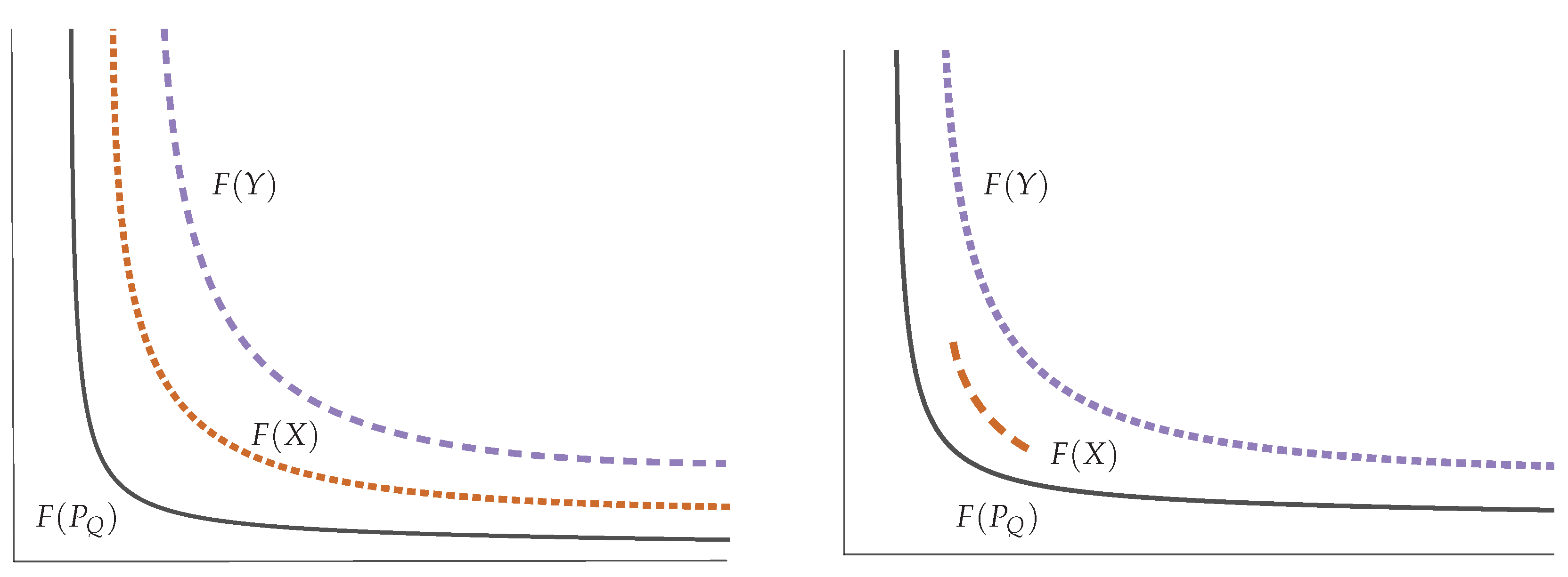
2.2. Multi-objective Optimization

As an application of the $(p,q)$-distances, we will consider in this work continuous multi-objective optimization problems (MOPs). Problems of this kind can be expressed mathematically as

$$\min \{F\left(x\right):x\in Q\subset {\mathbb{R}}^n\},$$

(2)

where the function F is defined as a vector of objective functions

$$F:Q\subset {\mathbb{R}}^n\to {\mathbb{R}}^k,F\left(x\right):=(f_1\left(x\right),\dots ,f_k\left(x\right)).$$

We will assume here that all objectives $f_i:X\to \mathbb{R}$, for $i\in \{1,\dots k\}$, are continuous. The optimality of MOPs is typically defined via the concept of dominance (see [31]).

Definition 1.

In the context of MOPs the following are standard notions:

(i)

Let $v=(v_1,\dots ,v_k)$ and $w=(w_1,\dots ,w_k)\in {\mathbb{R}}^k$. Then the vector v is less than w (denoted $v{<}_{\mathrm{p}}w$), if $v_i<w_i$ for all $i\in \{1,\dots ,k\}$. The relation ${⩽}_{\mathrm{p}}$ is defined analogously.

(ii)

A vector $y\in Q$ is dominated by a vector $x\in Q$ (in short: $x\prec y$) with respect to (2) if $F\left(x\right){⩽}_{\mathrm{p}}F\left(y\right)$ and $F\left(x\right)\ne F\left(y\right)$, i.e., there exists a $j\in \{1,\dots ,k\}$ such that $f_j\left(x\right)<f_j\left(y\right)$.

(iii)

A point $x\in Q$ is called Pareto optimal or a Pareto point if there is no $y\in Q$ which dominates x.

(iv)

The set of all Pareto optimal solutions is called the Pareto set, denoted by $P_Q$.

(v)

The image of the Pareto set, $F\left(P_Q\right)$, is called the Pareto front.

It is known that under certain mild smoothness assumptions the Pareto set and the Pareto front define $(k-1)$-dimensional objects [32]. Hence, for set oriented solvers such as cell mapping, subdivision techniques, and evolutionary algorithms, the question naturally arises as to how to measure the approximation quality of the obtained solution set with respect to the Pareto set/front. To accomplish this task, several performance indicators have been proposed in the specialized literature. There exist, for instance, the hypervolume indicator [21,33], the R2 indicator [34], the IGD${}^{+}$ [35], and the DOA [36]. Moreover, in the context of multi-criteria decision-making processes, the properties of some distance measures, as the Hamming, Euclidean, and Hausdorff metrics, is investigated in [37,38]. In this work, we will focus on a new variant of the Hausdorff distance [6]. For convenience of the reader, we recall in the following the most important definitions.

Definition 2.

Let $u,v\in {\mathbb{R}}^n$, arbitrary $A,B\subset {\mathbb{R}}^n$, and $\parallel ·\parallel$ be a vector norm. The Hausdorff distance $d_H(·,·)$ is defined as follows:

(i)

$\mathrm{dist}(u,A):=\inf \{\parallel u-v\parallel :v\in A\}$,

(ii)

$\mathrm{dist}(B,A):=\sup \left\{\mathrm{dist}\right(u,A):u\in B\}$,

(iii)

$d_H(A,B):=\max \left\{\mathrm{dist}\right(A,B),\mathrm{dist}(B,A\left)\right\}$.

The Hausdorff distance $d_H$ is widely used in many fields. It is, however, of limited practical use when measuring the distance of the outcome of a stochastic search method such as an evolutionary algorithm to the Pareto set/front. The main reason for this is that evolutionary algorithms may generate outliers that are punished too strongly by $d_H$. As a remedy, the averaged Hausdorff distance has been proposed in [14]. In this study the vector norm is the 2-norm, i.e., the Euclidean norm.

Definition 3

(Schütze et al. [14]). For $p\in \mathbb{N}$, and finite sets $A,B\subset {\mathbb{R}}^n$ the value

$${\Delta }_p(A,B):=\max \{{\mathrm{GD}}_p(A,B),{\mathrm{IGD}}_p(A,B)\},$$

where

$${\mathrm{GD}}_p(A,B):={\left(\frac{1}{\left|A\right|}\sum _{a\in A}d{(a,B)}^p\right)}^{\frac{1}{p}}and{\mathrm{IGD}}_p(A,B):={\left(\frac{1}{\left|B\right|}\sum _{b\in B}d{(b,A)}^p\right)}^{\frac{1}{p}},$$

is called the averaged Hausdorff distance between A and B.

The indicator ${\Delta }_p$ can be viewed as a composition of slight variations of the Generational Distance (GD, see [39]) and the Inverted Generational Distance (IGD, see [40]). It is ${\Delta }_{\infty }=d_H$, but for finite values of p the indicator ${\Delta }_p$ averages the distances considered in $d_H$. More precisely, the larger the value of p, the harder single outliers will be punished by ${\Delta }_p$. Hence, as opposed to $d_H$, the distance ${\Delta }_p$ does not punish single (or few) outliers in a candidate set. For more discussion about ${\Delta }_p$ and its relation to other indicators we refer to [14,41].

Definition 4

(Vargas–Bogoya [26]). For $p,q\in {\mathbb{R}}^{\times }$, and finite sets $A,B\subset {\mathbb{R}}^n$ the value

$${\Delta }_{p,q}(A,B):=\max \{{\mathrm{GD}}_{p,q}(A,B\backslash A),{\mathrm{GD}}_{p,q}(B,A\backslash B)\},$$

where ${\displaystyle {\mathrm{GD}}_{p,q}(A,B):={\left(\frac{1}{\left|A\right|}\sum _{a\in A}{\left(\frac{1}{\left|B\right|}\sum _{b\in B}d{(a,b)}^q\right)}^{\frac{p}{q}}\right)}^{\frac{1}{p}}}$ is called the $(p,q)$-averaged Hausdorff distance between A and B.

For finite sets, the indicator ${\Delta }_{p,q}$, introduced in [26] was also defined for p or $q=0$, and even for p or $q=\pm \infty$. It is a generalization of ${\Delta }_p$ in the sense that between disjoint subsets we have

$$\underset{q\to -\infty }{\lim }{\Delta }_{p,q}={\Delta }_p.$$

The parameters p and q can be independently modified in order to produce customary spread archives (depending on q) located with customary closeness (depending on p) to the Pareto front.

Finally, let us recall that one characteristic of a performance indicator is Pareto compliance: for two subsets A and B we say that $A⪯B$ if for every $b\in B$ there exists an element $a\in A$ such that $a⪯b$. If this does not hold, we write $A⋠B$. We say that a performance indicator $\mathcal{I}$ is Pareto compliant if for any two sets A and B with $A⪯B$ and $B⋠A$ it follows $\mathcal{I}\left(A\right)⩽\mathcal{I}\left(B\right)$. We refer to [42] for details.

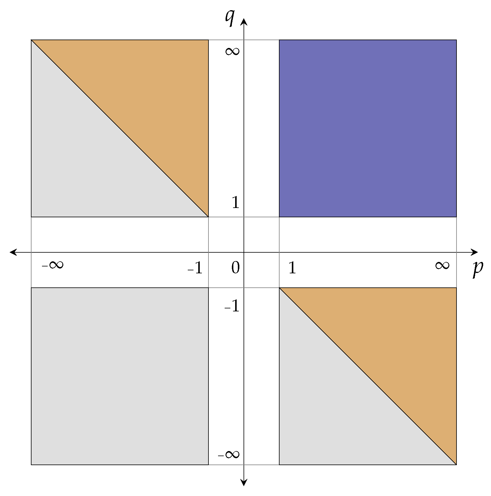
3. The $(\mathit{p},\mathit{q})$-Averaged Hausdorff Distance for Measurable Sets

3.1. Properties of Integral Power Means

We start summarizing some fundamental properties of integral power means that we will need for our subsequent calculations.

Theorem 1.

Let X and Y denote finite-measure spaces, $f,g:X\to [0,\infty )$ non-negative measurable functions, and $d:X\times Y\to [0,\infty )$ a measurable function with respect to the product measure on $X\times Y$. The integral power mean $\mathcal{M}$ satisfies the following properties:

(i)

If $p\in \overline{\mathbb{R}}$ and $k\in [0,\infty )$, then $\underset{x\in X}{{\mathcal{M}}^p}\left(k\right)=k$ and $\underset{x\in X}{{\mathcal{M}}^p}\left(kf\left(x\right)\right)=k\underset{x\in X}{{\mathcal{M}}^p}\left(f\left(x\right)\right)$.

(ii)

For any $p\in \overline{\mathbb{R}}$, we have $\underset{x\in X}{{\mathcal{M}}^p}\left(\underset{y\in Y}{{\mathcal{M}}^p}\left(d(x,y)\right)\right)=\underset{y\in Y}{{\mathcal{M}}^p}\left(\underset{x\in X}{{\mathcal{M}}^p}\left(d(x,y)\right)\right)$.

(iii)

If $1⩽p⩽\infty$, then $\underset{x\in X}{{\mathcal{M}}^p}(f\left(x\right)+g\left(x\right))⩽\underset{x\in X}{{\mathcal{M}}^p}\left(f\left(x\right)\right)+\underset{x\in X}{{\mathcal{M}}^p}\left(g\left(x\right)\right)$.

(iv)

If $p\in \overline{\mathbb{R}}$ and $f\left(x\right)⩽g\left(x\right)$ for all $x\in X$, then $\underset{x\in X}{{\mathcal{M}}^p}\left(f\left(x\right)\right)⩽\underset{x\in X}{{\mathcal{M}}^p}\left(g\left(x\right)\right)$.

(v)

For $p,q\in \overline{\mathbb{R}}$ with $0<p⩽q$, we have that $\underset{x\in X}{{\mathcal{M}}^p}\left(f\left(x\right)\right)⩽\underset{x\in X}{{\mathcal{M}}^q}\left(f\left(x\right)\right)$.

Proof. 

The proofs of (i) and (ii) are straightforward. To prove (iii) we only need the Minkowski inequality,

$$\begin{array}{cc}\hfill \underset{x\in X}{{\mathcal{M}}^p}(f\left(x\right)+g\left(x\right))& =\mu {\left(X\right)}^{-\frac{1}{p}}{\parallel f+g\parallel }_p\hfill \\ \hfill & ⩽\mu {\left(X\right)}^{-\frac{1}{p}}\left({\parallel f\parallel }_p+{\parallel g\parallel }_p\right)=\underset{x\in X}{{\mathcal{M}}^p}\left(f\left(x\right)\right)+\underset{x\in X}{{\mathcal{M}}^p}\left(g\left(x\right)\right).\hfill \end{array}$$

The proof of (iv) is also straightforward from the definitions and a simple proof of (v) can be given as a particular case of [43] (Theorem 3) which we recall here for completeness. For a positive real v, consider the function

$${\omega }_r\left(v\right):={\int }_1^v{t}^{r-1}dt=\left\{\begin{array}{cc}{\displaystyle \frac{v^r-1}{r},}\hfill & r\ne 0;\hfill \\ \log v,\hfill & r=0.\hfill \end{array}\right.$$

Since the function $t^u$, with t a positive constant and $u⩾0$ is increasing with respect to u, we easily get ${\omega }_r\left(v\right)⩽{\omega }_s\left(v\right)$ for $0⩽r⩽s$ and every $v⩾0$. Consider the following linear integral operator

$$\mathcal{J}[f]:=\frac{1}{\mu \left(X\right)}{\int }_{X}f\mathrm{d}\mu ={-\int }_{X}f\mathrm{d}\mu .$$

Assume first, that $p\ne 0$, then for any $x\in X$,

$$\begin{array}{cc}\hfill \mathcal{J}[{\omega }_p\left(\frac{f\left(x\right)}{\underset{}{{\mathcal{M}}^p}\left(f\left(X\right)\right)}\right)]& =\frac{1}{p}\left(\mathcal{J}[\frac{f\left(x\right)}{\underset{}{{\mathcal{M}}^p}\left(f\left(X\right)\right)}\right]{}^p-\mathcal{J}\left[1\right])\hfill \\ \hfill & =\frac{1}{p}\left(\frac{1}{{\left(\underset{}{{\mathcal{M}}^p}\left(f\left(X\right)\right)\right)}^p}{-\int }_X{f}^p\mathrm{d}\mu -{-\int }_X\mathrm{d}\mu \right)=0.\hfill \end{array}$$

Similarly, if $p=0$ we have

$$\begin{array}{cc}\hfill \mathcal{J}[{\omega }_0\left(\frac{f\left(x\right)}{\underset{}{{\mathcal{M}}^0}\left(f\left(X\right)\right)}\right)]& =\mathcal{J}[\log \left(f\left(x\right)\right)-\log \left(\underset{}{{\mathcal{M}}^0}\left(f\left(X\right)\right)\right]\hfill \\ \hfill & ={-\int }_X\log f\mathrm{d}\mu -\log ({\mathcal{M}}^0\left(f\left(X\right)\right)\mathcal{J}\left[1\right]=0.\hfill \end{array}$$

Suppose that $0⩽p<q$. Since ${\omega }_p(·)⩽{\omega }_q(·)$ implies $\mathcal{J}({\omega }_p(·))⩽\mathcal{J}({\omega }_q(·))$, we obtain

$$0⩽\mathcal{J}[{\omega }_q\left(\frac{f\left(x\right)}{\underset{}{{\mathcal{M}}^p}\left(f\left(X\right)\right)}\right)]=\frac{1}{q}\left[{\left(\frac{\underset{}{{\mathcal{M}}^q}\left(f\left(X\right)\right)}{\underset{}{{\mathcal{M}}^p}\left(f\left(X\right)\right)}\right)}^q-1\right],$$

from which it follows that $\underset{x\in X}{{\mathcal{M}}^p}\left(f\left(x\right)\right)⩽\underset{x\in X}{{\mathcal{M}}^q}\left(f\left(x\right)\right)$. □

3.2. Definition of ${\Delta }_{p,q}$ for Measurable Sets

With the aid of Theorem 1 we generalize the results of [26] (Section 3). For easy reference, we provide here slightly abbreviated but complete proofs. Given a metric measure space $(\mathsf{\Sigma },d,\mu )$, let $\mathfrak{M}\left(\mathsf{\Sigma }\right)$ denote the $\sigma$-algebra of all measurable subsets of $\mathsf{\Sigma }$ and let ${\mathfrak{M}}_{<\infty }\left(\mathsf{\Sigma }\right)$ refer to those elements of $\mathfrak{M}\left(\mathsf{\Sigma }\right)$ having finite measure. As it should be expected from the context, any set relation obtained from calculations involving an underlying measure $\mu$ should be understood to hold in a measure-theoretic sense, i.e., almost everywhere (a.e.). For example, for $X,Y\in {\mathfrak{M}}_{<\infty }\left(\mathsf{\Sigma }\right)$, a result saying $X=Y$, or $X\subset Y$ actually holds almost everywhere, which means that $\mu \{X\ne Y\}=0$, or $\mu \{X⊈Y\}=0$, respectively. Thus, it is convenient in this setting to identify a set $X\in {\mathfrak{M}}_{<\infty }\left(\mathsf{\Sigma }\right)$ with the whole equivalence class $\left[X\right]:=\{Y\mid X=Y,a.e.\}$, and think of these classes as the elements of ${\mathfrak{M}}_{<\infty }\left(\mathsf{\Sigma }\right)$ to remove the need for the a.e. abbreviation. Also, to avoid an overload of parentheses in the forthcoming expressions, the distance $d(x,y)$ between $x,y\in \mathsf{\Sigma }$ will be abbreviated by $d_{x,y}$.

Definition 5.

For $p,q\in {\mathbb{R}}^{\times }$, the generational $(p,q)$-distance ${\mathrm{GD}}_{p,q}(X,Y)$ between two sets $X,Y\in {\mathfrak{M}}_{<\infty }\left(\mathsf{\Sigma }\right)$ is given by

$${\mathrm{GD}}_{p,q}(X,Y):=\underset{x\in X}{{\mathcal{M}}^p}\left(\underset{y\in Y}{{\mathcal{M}}^q}\left(d_{x,y}\right)\right)={\left({-\int }_X{\left({-\int }_Y{d}_{x,y}^q\mathrm{d}y\right)}^{\frac{p}{q}}\mathrm{d}x\right)}^{\frac{1}{p}},$$

where the sets X and Y are implicitly assumed to be disjoint when $p<0$ or $q<0$.

As in the finite case, the definition of ${\mathrm{GD}}_{p,q}$ can be easily extended for $p,q\in \overline{\mathbb{R}}$, but still has two undesirable drawbacks, first ${\mathrm{GD}}_{p,q}(X,X)$ can be different from zero, and second, in general the values of ${\mathrm{GD}}_{p,q}(X,Y)$ and ${\mathrm{GD}}_{p,q}(Y,X)$ can be different, thus this indicator does not define a metric. To obtain a proper metric we introduce the following modification.

Definition 6.

The $(p,q)$-averaged Hausdorff distance is the map ${\Delta }_{p,q}:{\mathfrak{M}}_{<\infty }\left(\mathsf{\Sigma }\right)\times {\mathfrak{M}}_{<\infty }\left(\mathsf{\Sigma }\right)\to [0,\infty )$ given by

$${\Delta }_{p,q}(X,Y):=\max \{{\mathrm{GD}}_{p,q}(X,Y\backslash X),{\mathrm{GD}}_{p,q}(Y,X\backslash Y)\}.$$

Remark 1.

For finite subsets $X,Y\subset {\mathbb{R}}^n$ endowed with the standard counting measure μ, the previous notions of ${\mathrm{GD}}_{p,q}$ and ${\Delta }_{p,q}$ coincide with the ones in Definition 4.

Figure 1 illustrates how the shape of ${\Delta }_{p,q}$-metric balls $B_{\epsilon }:=\{x\in {\mathbb{R}}^2:{\Delta }_{p,q}(A,x)⩽\epsilon \}$ around a discrete set A of ten points (that approximates a segment of negative slope in the plane) varies as p and q take several different values. Notice that for negative values of p and q the balls’ shape resemble the shape of A and enclose all of its points.

3.3. Metric Properties

The extension of ${\Delta }_{p,q}$ to measurable sets given in Definition 6 preserves the nice metric properties of the finite version considered in [26] (Section 3). In particular, Theorem 1 enables us to show a result analogous to [26] (Theorem 3.3).

Theorem 2.

Suppose that $1⩽p,q<\infty$. Then the generational $(p,q)$-distance ${\mathrm{GD}}_{p,q}$ satisfies the triangle inequality, namely

$${\mathrm{GD}}_{p,q}(X,Z)⩽{\mathrm{GD}}_{p,q}(X,Y)+{\mathrm{GD}}_{p,q}(Y,Z)$$

for any sets $X,Y,Z\in {\mathfrak{M}}_{<\infty }\left(\mathsf{\Sigma }\right)$.

Proof. 

From the triangle inequality for the metric $d(·,·)$ we have

$$d_{x,z}⩽d_{x,y}+d_{y,z}(x\in X,y\in Y,z\in Z).$$

Taking the q-average over Z at both sides and using Theorem 1 (i)–(iii), yields

$$\underset{z\in Z}{{\mathcal{M}}^q}\left(d_{x,z}\right)⩽\underset{z\in Z}{{\mathcal{M}}^q}(d_{x,y}+d_{y,z})⩽\underset{z\in Z}{{\mathcal{M}}^q}\left(d_{x,y}\right)+\underset{z\in Z}{{\mathcal{M}}^q}\left(d_{y,z}\right)=d_{x,y}+\underset{z\in Z}{{\mathcal{M}}^q}\left(d_{y,z}\right).$$

(3)

Now, we consider two cases for the parameters $1⩽p,q<\infty$, independently.

Case $p⩽q$: Taking at both sides of (3) the p-average over X and using Theorem 1 (i), (iii), and (iv), we get

$$\underset{x\in X}{{\mathcal{M}}^p}\left(\underset{z\in Z}{{\mathcal{M}}^q}\left(d_{x,z}\right)\right)⩽\underset{x\in X}{{\mathcal{M}}^p}\left(d_{x,y}+\underset{z\in Z}{{\mathcal{M}}^q}\left(d_{y,z}\right)\right)=\underset{x\in X}{{\mathcal{M}}^p}\left(d_{x,y}\right)+\underset{z\in Z}{{\mathcal{M}}^q}\left(d_{y,z}\right).$$

(4)

In this expression, the LHS is precisely ${\mathrm{GD}}_{p,q}(X,Z)$ which does not depend on Y. We now take the p-average over Y at both sides of (4) and use Theorem 1 (i), (iii), and (iv), to obtain

$${\mathrm{GD}}_{p,q}(X,Z)⩽\underset{y\in Y}{{\mathcal{M}}^p}\left(\underset{x\in X}{{\mathcal{M}}^p}\left(d_{x,y}\right)+\underset{z\in Z}{{\mathcal{M}}^q}\left(d_{y,z}\right)\right)=\underset{y\in Y}{{\mathcal{M}}^p}\left(\underset{x\in X}{{\mathcal{M}}^p}\left(d_{x,y}\right)\right)+{\mathrm{GD}}_{p,q}(Y,Z).$$

To finish this case note that from Theorem 1 (ii), (iv), and (v), we have that

$$\underset{y\in Y}{{\mathcal{M}}^p}\left(\underset{x\in X}{{\mathcal{M}}^p}\left(d_{x,y}\right)\right)=\underset{x\in X}{{\mathcal{M}}^p}\left(\underset{y\in Y}{{\mathcal{M}}^p}\left(d_{x,y}\right)\right)⩽\underset{x\in X}{{\mathcal{M}}^p}\left(\underset{y\in Y}{{\mathcal{M}}^q}\left(d_{x,y}\right)\right)={\mathrm{GD}}_{p,q}(X,Y)$$

which proves the claim.

Case $q⩽p$: Here, we note that the LHS of (3) does not depend on Y, and take at both sides of (3) the q-average over Y. Hence, Theorem 1 (i), (iii)–(v) yield

$$\begin{array}{c}\hfill \underset{z\in Z}{{\mathcal{M}}^q}\left(d_{x,z}\right)⩽\underset{y\in Y}{{\mathcal{M}}^q}\left(d_{x,y}+\underset{z\in Z}{{\mathcal{M}}^q}\left(d_{y,z}\right)\right)⩽\underset{y\in Y}{{\mathcal{M}}^q}\left(d_{x,y}\right)+{\mathrm{GD}}_{p,q}(Y,Z).\end{array}$$

Lastly, we take the p-average over X and use Theorem 1 (ii)–(iv), to obtain

$${\mathrm{GD}}_{p,q}(X,Z)⩽\underset{x\in X}{{\mathcal{M}}^p}\left(\underset{y\in Y}{{\mathcal{M}}^q}\left(d_{x,y}\right)+{\mathrm{GD}}_{p,q}(Y,Z)\right)={\mathrm{GD}}_{p,q}(X,Z)+{\mathrm{GD}}_{p,q}(Y,Z),$$

which is the required result. □

Corollary 1.

For $p,q\in {\mathbb{R}}^{\times }$ the $(p,q)$-averaged Hausdorff distance ${\Delta }_{p,q}$ is a semimetric on the collection ${\mathfrak{M}}_{<\infty }\left(\mathsf{\Sigma }\right)$ of all measurable subsets of Σ with finite measure. Moreover, between disjoint sets, ${\Delta }_{p,q}$ is a proper metric on ${\mathfrak{M}}_{<\infty }\left(\mathsf{\Sigma }\right)$ for $1⩽p,q<\infty$.

Proof. 

Definition 6 easily implies that ${\Delta }_{p,q}(·,·)⩾0$ as well as ${\Delta }_{p,q}(X,Y)={\Delta }_{p,q}(Y,X)$, for every pair $X,Y\in {\mathfrak{M}}_{<\infty }\left(\mathsf{\Sigma }\right)$ and all $p,q\in {\mathbb{R}}^{\times }$. From Definition 5 we can see that ${\mathrm{GD}}_{p,q}(X,Y\backslash X)=0$ if and only if $X=⌀$ or $Y\subseteq X$ (and hence $Y\backslash X=⌀$). We thus find, for $X,Y\ne ⌀$, that

$${\Delta }_{p,q}(X,Y)=0\mathrm{if}\mathrm{and}\mathrm{only}\mathrm{if}X=Y.$$

We have shown that ${\Delta }_{p,q}$ is a semimetric on ${\mathfrak{M}}_{<\infty }\left(\mathsf{\Sigma }\right)$, and since the maximum of two functions satisfying the triangle inequality also satisfies it, Theorem 2 shows that ${\Delta }_{p,q}$ satisfies the triangle inequality when $1⩽p,q<\infty$. □

Theorem 3.

Suppose that for any sets $X,Y,Z\in {\mathfrak{M}}_{<\infty }\left(\mathsf{\Sigma }\right)$ there exist some constants $0<r<R$ such that $r⩽d_{u,v}⩽R$ holds for all pairs $(u,v)$ in $X\times Y$, $X\times Z$, or $Y\times Z$. Then, for all non-simultaneously positive $p,q\in {\mathbb{R}}^{\times }$ with $\left|p\right|,\left|q\right|⩾1$ the generational $(p,q)$-distance ${\mathrm{GD}}_{p,q}$ satisfies the following relaxed triangle inequality

$${\mathrm{GD}}_{p,q}(X,Z)⩽\frac{R^2}{r^2}\left({\mathrm{GD}}_{p,q}(X,Y)+{\mathrm{GD}}_{p,q}(Y,Z)\right).$$

Proof. 

We prove the theorem in three steps.

Step 1: Take $p\in {\mathbb{R}}^{\times }$ and assume that $q<0$, we will show that

$${\mathrm{GD}}_{p,\left|q\right|}(X,Y)⩽\frac{R}{r}{\mathrm{GD}}_{p,q}(X,Y).$$

(5)

For any $x\in X$ and all $y_1,y_2\in Y$ we have $\frac{r}{R}⩽\frac{d_{x,y_1}}{d_{x,y_2}}⩽\frac{R}{r}$, thus

$$\frac{R}{r}⩾{\left({-\int }_Y{-\int }_Y{\left[\frac{d_{x,y_1}}{d_{x,y_2}}\right]}^{\left|q\right|}\mathrm{d}{y}_1\mathrm{d}{y}_2\right)}^{\frac{1}{\left|q\right|}}={\left({-\int }_Y{d}_{x,y_1}^{\left|q\right|}\mathrm{d}{y}_1\right)}^{\frac{1}{\left|q\right|}}{\left({-\int }_Y{d}_{x,y_2}^{-\left|q\right|}\mathrm{d}{y}_2\right)}^{\frac{1}{\left|q\right|}}.$$

Using the fact that $q=-\left|q\right|$, we get

$${\left({-\int }_Y{d}_{x,y_1}^{\left|q\right|}\mathrm{d}{y}_1\right)}^{\frac{1}{\left|q\right|}}⩽\frac{R}{r}{\left({-\int }_Y{d}_{x,y_2}^q\mathrm{d}{y}_2\right)}^{\frac{1}{q}},$$

which by (1), proves that $\underset{y\in Y}{{\mathcal{M}}^{\left|q\right|}}\left(d_{x,y}\right)⩽\frac{R}{r}\underset{y\in Y}{{\mathcal{M}}^q}\left(d_{x,y}\right)$. Calculating the p-average $\underset{x\in X}{{\mathcal{M}}^p}$ of both sides, and from Theorem 1 (i) and (iv), we finally get $\underset{x\in X}{{\mathcal{M}}^p}\left(\underset{y\in Y}{{\mathcal{M}}^{\left|q\right|}}\left(d_{x,y}\right)\right)⩽\frac{R}{r}\underset{x\in X}{{\mathcal{M}}^p}\left(\underset{y\in Y}{{\mathcal{M}}^q}\left(d_{x,y}\right)\right),$ which, by Definition 5, is precisely (5).

Step 2: Now, take $q\in {\mathbb{R}}^{\times }$ and assume that $p<0$, we will show that

$${\mathrm{GD}}_{\left|p\right|,q}(X,Y)⩽\frac{R}{r}{\mathrm{GD}}_{p,q}(X,Y).$$

(6)

By hypothesis, for any $y\in Y$ and all $x_1,x_2\in X$ we have $\frac{r}{R}⩽\frac{d_{x_1,y}}{d_{x_2,y}}⩽\frac{R}{r}$. Therefore, proceeding as before and applying again Theorem 1 (i) and (iv) we conclude that $\underset{y\in Y}{{\mathcal{M}}^q}\left(d_{x_1,y}\right)⩽\frac{R}{r}\underset{y\in Y}{{\mathcal{M}}^q}\left(d_{x_2,y}\right)$. Hence,

$${\left({-\int }_X{\left(\underset{y\in Y}{{\mathcal{M}}^q}\left(d_{x_1,y}\right)\right)}^{\left|p\right|}\mathrm{d}{x}_1\right)}^{\frac{1}{\left|p\right|}}{\left({-\int }_X{\left(\underset{y\in Y}{{\mathcal{M}}^q}\left(d_{x_2,y}\right)\right)}^p\mathrm{d}{x}_2\right)}^{\frac{1}{\left|p\right|}}={\left({-\int }_X{-\int }_X{\left[\frac{\underset{y\in Y}{{\mathcal{M}}^q}\left(d_{x_1,y}\right)}{\underset{y\in Y}{{\mathcal{M}}^q}\left(d_{x_2,y}\right)}\right]}^{\left|p\right|}\mathrm{d}{x}_1\mathrm{d}{x}_2\right)}^{\frac{1}{\left|p\right|}}⩽\frac{R}{r},$$

from which we deduce

$${\left({-\int }_X{\left(\underset{y\in Y}{{\mathcal{M}}^q}\left(d_{x_1,y}\right)\right)}^{\left|p\right|}\mathrm{d}{x}_1\right)}^{\frac{1}{\left|p\right|}}⩽\frac{R}{r}{\left({-\int }_X{\left(\underset{y\in Y}{{\mathcal{M}}^q}\left(d_{x_2,y}\right)\right)}^p\mathrm{d}{x}_2\right)}^{\frac{1}{p}}.$$

Using (1), the previous inequality can be written as

$$\underset{x\in X}{{\mathcal{M}}^{\left|p\right|}}\left(\underset{y\in Y}{{\mathcal{M}}^q}\left(d_{x,y}\right)\right)⩽\frac{R}{r}\underset{x\in X}{{\mathcal{M}}^p}\left(\underset{y\in Y}{{\mathcal{M}}^q}\left(d_{x,y}\right)\right),$$

which, by Definition 5, is precisely (6).

Step 3: From the previous two steps we easily obtain

$${\mathrm{GD}}_{\left|p\right|,\left|q\right|}(X,Y)⩽\frac{R}{r}{\mathrm{GD}}_{\left|p\right|,q}(X,Y)⩽\frac{R^2}{r^2}{\mathrm{GD}}_{p,q}(X,Y).$$

(7)

Theorem 1 (iv) and Definition 5 imply that ${\mathrm{GD}}_{p,q}(X,Z)⩽{\mathrm{GD}}_{\left|p\right|,\left|q\right|}(X,Z)$. Finally, the triangle inequality for ${\mathrm{GD}}_{\left|p\right|,\left|q\right|}$ (Theorem 2) and (7), produces the desired relation

$${\mathrm{GD}}_{p,q}(X,Z)⩽{\mathrm{GD}}_{\left|p\right|,\left|q\right|}(X,Y)+{\mathrm{GD}}_{\left|p\right|,\left|q\right|}(Y,Z)⩽\frac{R^2}{r^2}\left({\mathrm{GD}}_{p,q}(X,Y)+{\mathrm{GD}}_{p,q}(Y,Z)\right).$$

 □

Remark 2.

When the pair $(p,q)$ lies in the light-gray or violet regions of Figure 2, the distance ${\mathrm{GD}}_{p,q}$ satisfies a relaxed triangle inequality, with the drawback that the constant $R^2/r^2$ depends on the condition that $r⩽d_{u,v}⩽R$, for all pairs $(u,v)\in X\times Y$, $X\times Z$, or $Y\times Z$. For bounded and separated sets this condition always holds, and on those sets the associated $(p,q)$-averaged Hausdorff distance ${\Delta }_{p,q}$ becomes an inframetric as the following corollary implies.

Corollary 2.

Under the same hypothesis of Theorem 3 we have

$${\Delta }_{p,q}(X,Z)⩽\frac{R^2}{r^2}\left({\Delta }_{p,q}(X,Y)+{\Delta }_{p,q}(Y,Z)\right).$$

Proof. 

It follows immediately from Theorem 3 and Definition 6. □

Theorem 4.

Let $X,Y\in {\mathfrak{M}}_{<\infty }\left(\mathsf{\Sigma }\right)$ and suppose that $p,p^{\prime },q,q^{\prime }\in \overline{\mathbb{R}}$ satisfy $p⩽p^{\prime }$ and $q⩽q^{\prime }$. Then

$${\Delta }_{p,q}(X,Y)⩽{\Delta }_{p^{\prime },q}(X,Y)and{\Delta }_{p,q}(X,Y)⩽{\Delta }_{p,q^{\prime }}(X,Y).$$

Proof. 

It follows easily from Theorem 1 (v) and Definition 6. □

3.4. Pareto-Compliance

We return now to the setting of MOPs to consider the behavior of the generalized ${\mathrm{GD}}_{p,q}$ and ${\Delta }_{p,q}$ distances as performance indicators by studying their Pareto-compliance. A discussion of the Pareto-compliance for the indicators ${\mathrm{GD}}_p$ and ${\Delta }_p$ appeared in [14] (Section 3). Similar observations are valid for these new $(p,q)$-indicators, but a detailed and complete account of the details is part of ongoing research and will appear elsewhere. Here, as a first approach to the compliance question we present a basic result that describes the behavior of the indicator ${\mathrm{GD}}_{p,q}$ under stronger assumptions than the compliance notion mentioned at the end of Section 2.2.

Let us assume that given a decision space $Q\subset {\mathbb{R}}^n$, a MOP has an associated objective function $F:Q\to {\mathbb{R}}^k$, with objective space $F\left(Q\right)\subset {\mathbb{R}}^k$ endowed with the Euclidean distance $d(·,·)$ and the inherited Lebesgue measure $\mu$. Furthermore, let $P_Q$ denote the Pareto set and $F\left(P_Q\right)\subset {\mathbb{R}}^k$ the corresponding Pareto front. If $X\subset Q$ denotes an approximating subset (or archive), the explicit ${\mathrm{GD}}_{p,q}$-performance indicators assigned to X is given by

$${\mathcal{I}}_{p,q}^{\mathrm{GD}}\left(X\right):={\mathrm{GD}}_{p,q}(F\left(X\right),F\left(P_Q\right)).$$

For the following statement, let us recall here that a partition of a set X is a collection of disjoint and non-empty subsets of X whose union is the whole of X. Furthermore, for any $q\in \overline{\mathbb{R}}$ we abbreviate the q-averaged distance of $F\left(u\right)\in F\left(Q\right)$ to the Pareto front $F\left(P_Q\right)$ by ${\delta }_q\left(u\right):=\underset{v\in P_Q}{{\mathcal{M}}^q}\left(d(F\left(u\right),F\left(v\right))\right)$.

Theorem 5.

Suppose that for fixed $p,q\in \overline{\mathbb{R}}$ a pair of measurable archives $X,Y\subset Q$, satisfy that:

(i)

X and Y admit finite partitions $X={⨆}_{i=1}^m{X}_i$ and $Y={⨆}_{i=1}^m{Y}_i$ such that for each $i\in \{1,\dots ,m\}$:

(a)

$X_i\subset X$ and $Y_i\subset Y$ are subsets of non-null finite measure.

(b)

$\forall x\in X_i$, $\forall y\in Y_i$: $x⪯y$,

(ii)

$\forall x\in X$, $\forall y\in Y$: if $x⪯y\Rightarrow {\delta }_q\left(x\right)⩽{\delta }_q\left(y\right)$.

Then ${\mathcal{I}}_{p,q}^{\mathrm{GD}}\left(X\right)⩽{\mathcal{I}}_{p,q}^{\mathrm{GD}}\left(Y\right)$.

Proof. 

From condition (i) the archives X and Y admit partitions into the same number m of subsets and from (ii) it is clear that for any $i\in \{1,\dots ,m\}$ if $x\in X_i$ and $y\in Y_i$ then ${\delta }_q\left(x\right)⩽{\delta }_q\left(y\right)$. Hence, taking integral p-averages over $X_i$, and then over $Y_i$ of the quantities at both sides of this inequality we obtain for each i that

$$a_i^p:=\frac{1}{|X_i|}{\int }_{X_i}{\delta }_q{\left(x\right)}^p\mathrm{d}x⩽\frac{1}{|Y_i|}{\int }_{Y_i}{\delta }_q{\left(y\right)}^p\mathrm{d}y=:b_i^p.$$

(8)

Now, for each $i\in \{1,\dots ,m\}$ for which the inequality $\frac{|X_i|}{\left|X\right|}⩽\frac{|Y_i|}{\left|Y\right|}$ does not hold, we can further subdivide $X_i$ into a sufficiently large partition of $m_i$ non-null finite measure subsets $X_{i,1},X_{i,2},\dots ,X_{i,m_i}$, so that for all $j\in \{1,\dots ,m_i\}$ we can guarantee that

$$w_{i,j}:=\frac{|X_{i,j}|}{\left|X\right|}⩽\frac{|Y_i|}{\left|Y\right|}{\tilde{w}}_i.$$

(9)

Please note that this should be possible due to the assumption that $X_i$ has non-null finite measure. Since part (b) of condition (i) still holds for these subsets, (i.e., $\forall x\in X_{i,j}$, $\forall y\in Y_i$: $x⪯y$), an analogous relation to Inequality (8) is valid for them. Explicitly, for each $i\in \{1,\dots ,n\}$ and all $j\in \{1,\dots ,m_i\}$ we have

$$a_{i,j}^p:=\frac{1}{|X_{i,j}|}{\int }_{X_{i,j}}{\delta }_q{\left(x\right)}^p\mathrm{d}x⩽\frac{1}{|Y_i|}{\int }_{Y_i}{\delta }_q{\left(y\right)}^p\mathrm{d}y=:b_i^p.$$

Due to the chosen partitions of X and Y, it is clear that $\left|X\right|={\sum }_{i=1}^m\left|X_i\right|$, where $|X_i|={\sum }_{j=1}^{m_i}\left|X_{i,j}\right|$, and $\left|Y\right|={\sum }_{i=1}^m\left|Y_i\right|$. Therefore, with the notation of (9) it follows ${\sum }_{i=1}^m{\sum }_{j=1}^{m_i}{w}_{i,j}={\sum }_{i=1}^m{\tilde{w}}_i=1,$ which implies that the quantities $w_{i,j}$ and ${\tilde{w}}_i$ can be regarded as normalized weights appropriate for taking weighted averages. Using that $0⩽a_{i,j}⩽b_i$ and $0⩽w_{i,j}⩽{\tilde{w}}_i⩽1$, simple properties of (discrete) weighted power means ensure that ${\sum }_{i=1}^m{\sum }_{j=1}^{m_i}{w}_{i,j}{a}_{i,j}^p⩽{\sum }_{i=1}^m{\tilde{w}}_i{b}_i^p$. Thus, we can finally write

$$\begin{array}{cc}\hfill {\mathcal{I}}_{p,q}^{\mathrm{GD}}{\left(Y\right)}^p& =\frac{1}{\left|X\right|}\sum _{i=1}^m\sum _{j=1}^{m_i}{\int }_{X_{i,j}}{\delta }_q{\left(x\right)}^p\mathrm{d}x=\sum _{i=1}^m\sum _{j=1}^{m_j}\frac{|X_{i,j}|}{\left|X\right|}{a}_{i,j}^p=\sum _{i=1}^m\sum _{j=1}^{m_i}{w}_{i,j}{a}_{i,j}^p\hfill \\ \hfill & ⩽\sum _{i=1}^m{\tilde{w}}_i{b}_i^p=\sum _{i=1}^m\frac{|Y_i|}{\left|Y\right|}{b}_i^p=\frac{1}{\left|Y\right|}\sum _{i=1}^m{\int }_{Y_i}{\delta }_q{\left(y\right)}^p\mathrm{d}y={\mathcal{I}}_{p,q}^{\mathrm{GD}}{\left(Y\right)}^p,\hfill \end{array}$$

proving the statement. □

Remark 3.

Condition (i) of Theorem 5 implies the simpler (and weaker) dominance conditions:

(a’)

$X⪯Y$ (i.e., $\forall y\in Y$, $\exists x\in X$ such that $x⪯y$), and

(b’)

$\forall x\in X$, $\exists y\in Y$ such that $x⪯y$.

In many simple examples for which (a’) and (b’) hold, it is not difficult to find the partitions needed for Theorem 5 (i), however this is not always possible, and the question of when such partitions exist will not be considered here. Figure 3, show examples where (a’) and (b’) hold and the inequality ${\mathcal{I}}_{p,q}^{\mathrm{GD}}\left(X\right)⩽{\mathcal{I}}_{p,q}^{\mathrm{GD}}\left(Y\right)$ is both, true (left) and false (right). In these cases it can be shown that X and Y satisfy (left), and do not satisfy (right) the requirements of Theorem 5 (i), respectively.

Remark 4.

Another important observation is that condition (ii) of Theorem 5 allows for some freedom in the choice of an appropriate $q\in \overline{\mathbb{R}}$ such that the inequality ${\delta }_q\left(x\right)⩽{\delta }_q\left(y\right)$ holds for $x⪯y$, ensuring the compliance to Pareto optimality. This freedom is not available for the indicator ${\mathrm{GD}}_p$ because in that case ${\delta }_q\left(x\right)$ should be replaced by the corresponding quantity when $q\to \infty$ which is the standard distance from a set to a point $d(F\left(x\right),F\left(P_Q\right))$. The possibility to choose a value of q according to the problem is clearly an advantage, and provides an argument in favor of the generalized version ${\mathrm{GD}}_{p,q}$.

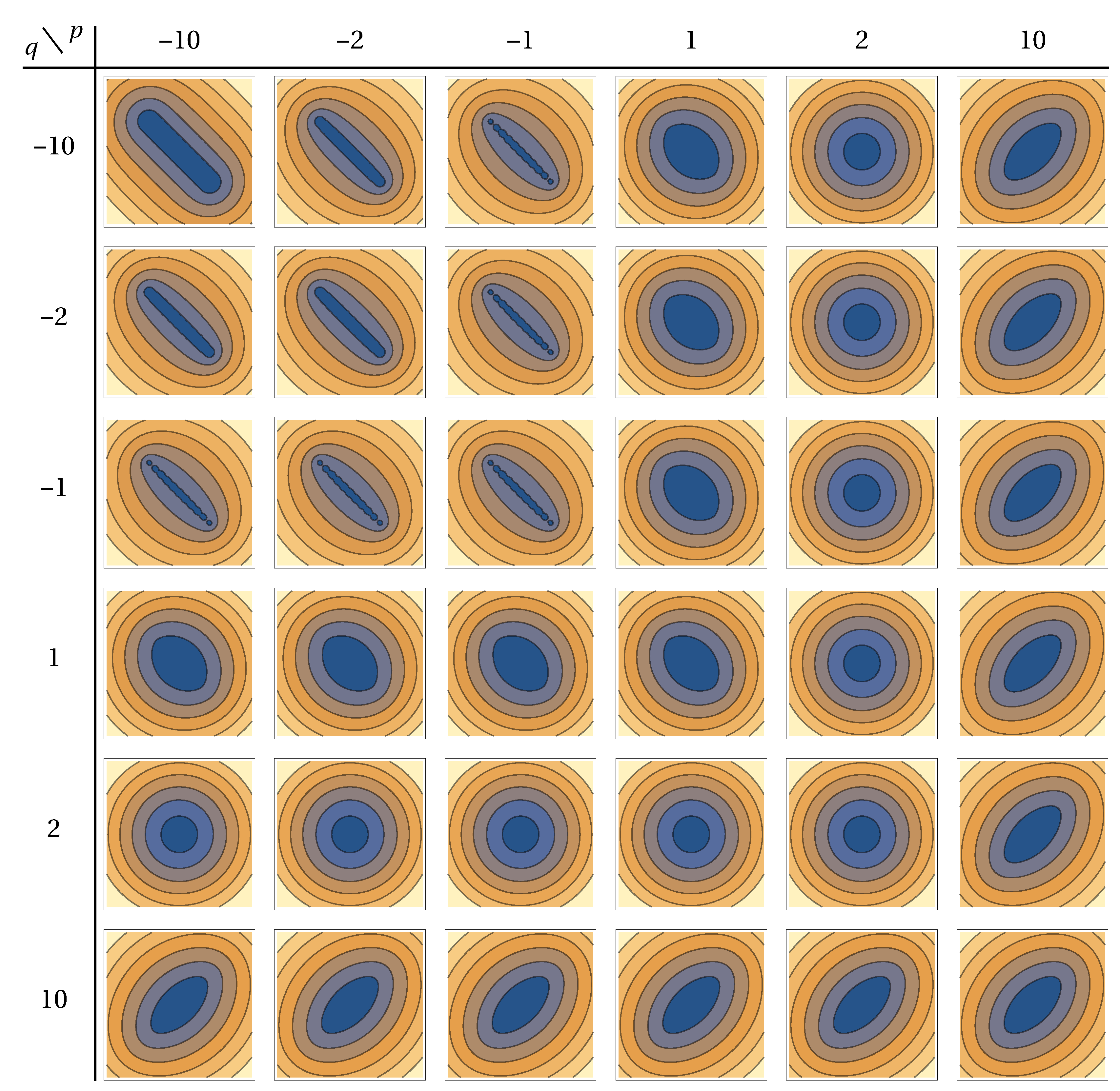
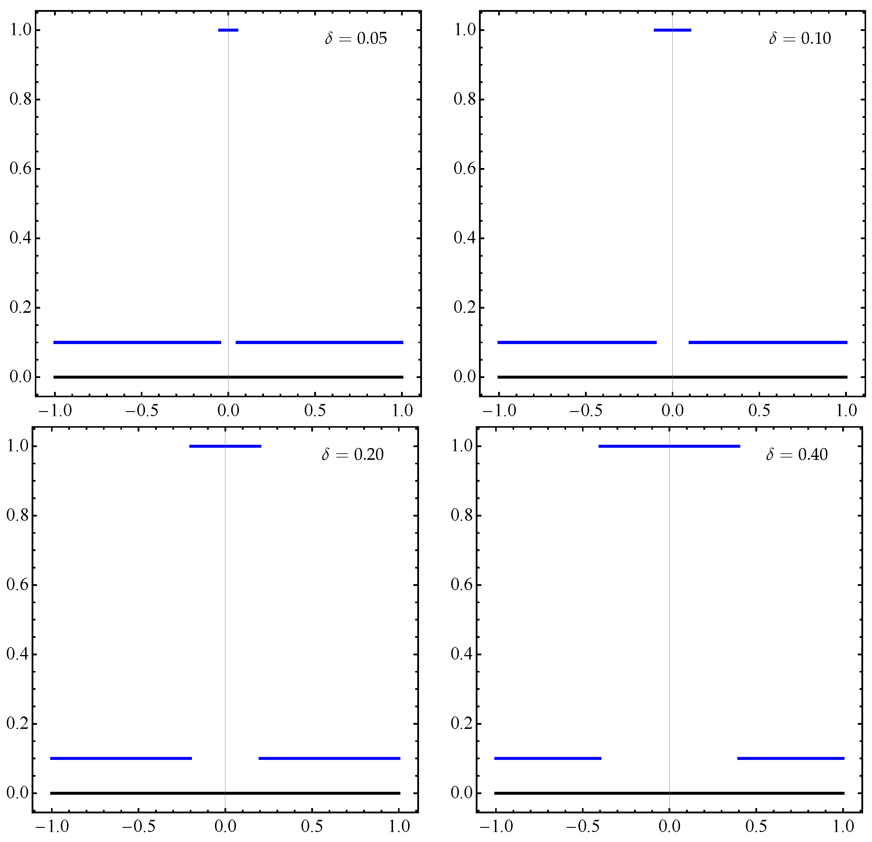
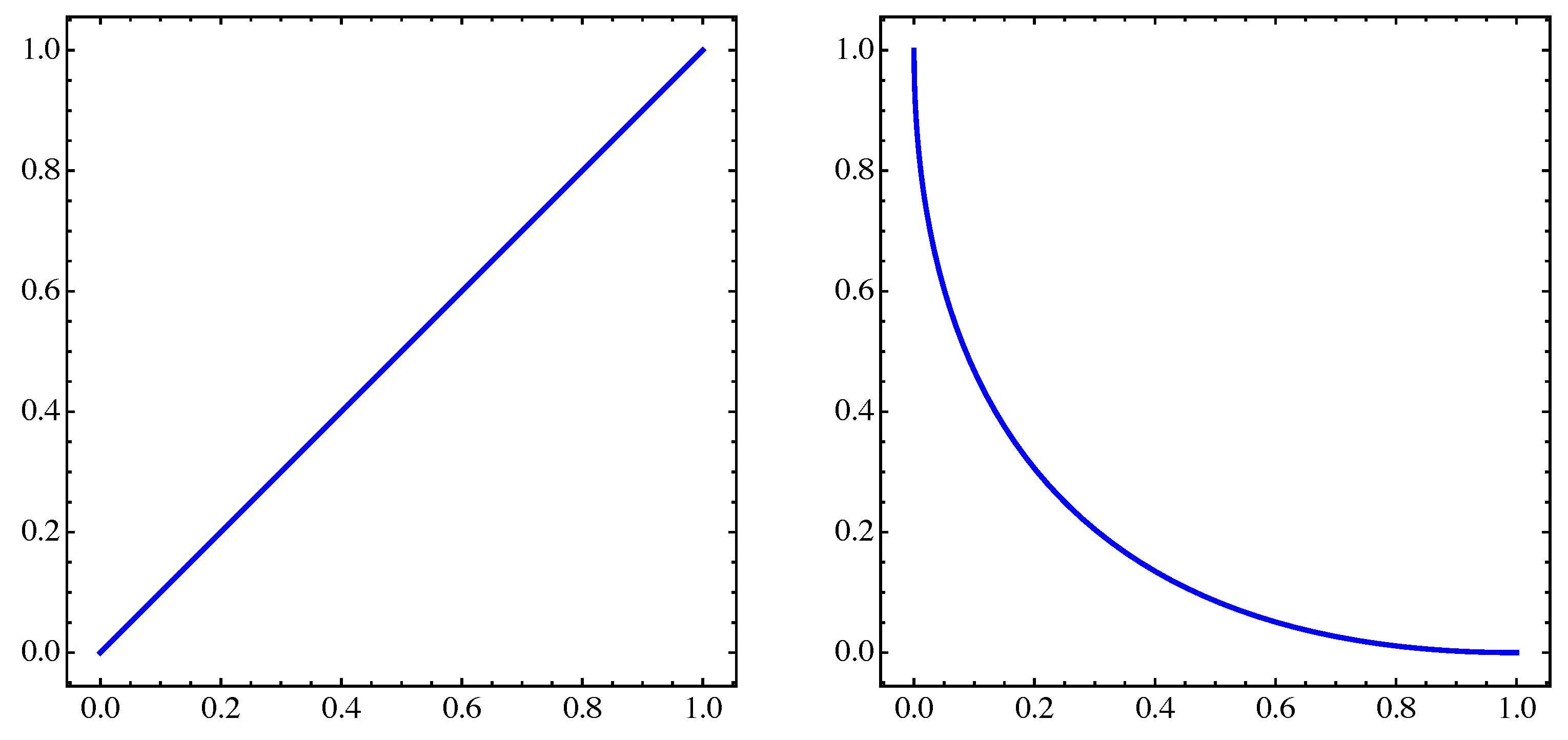
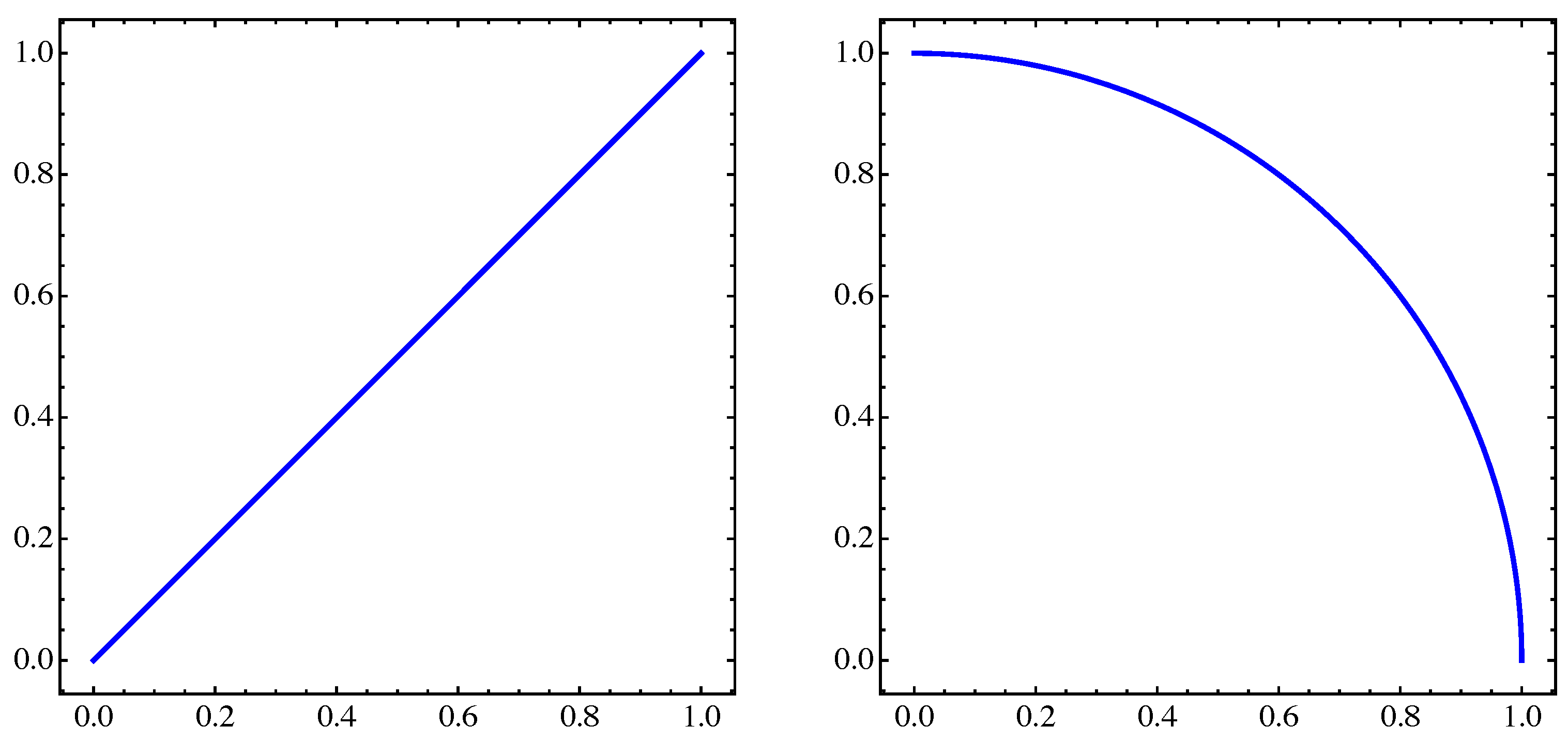
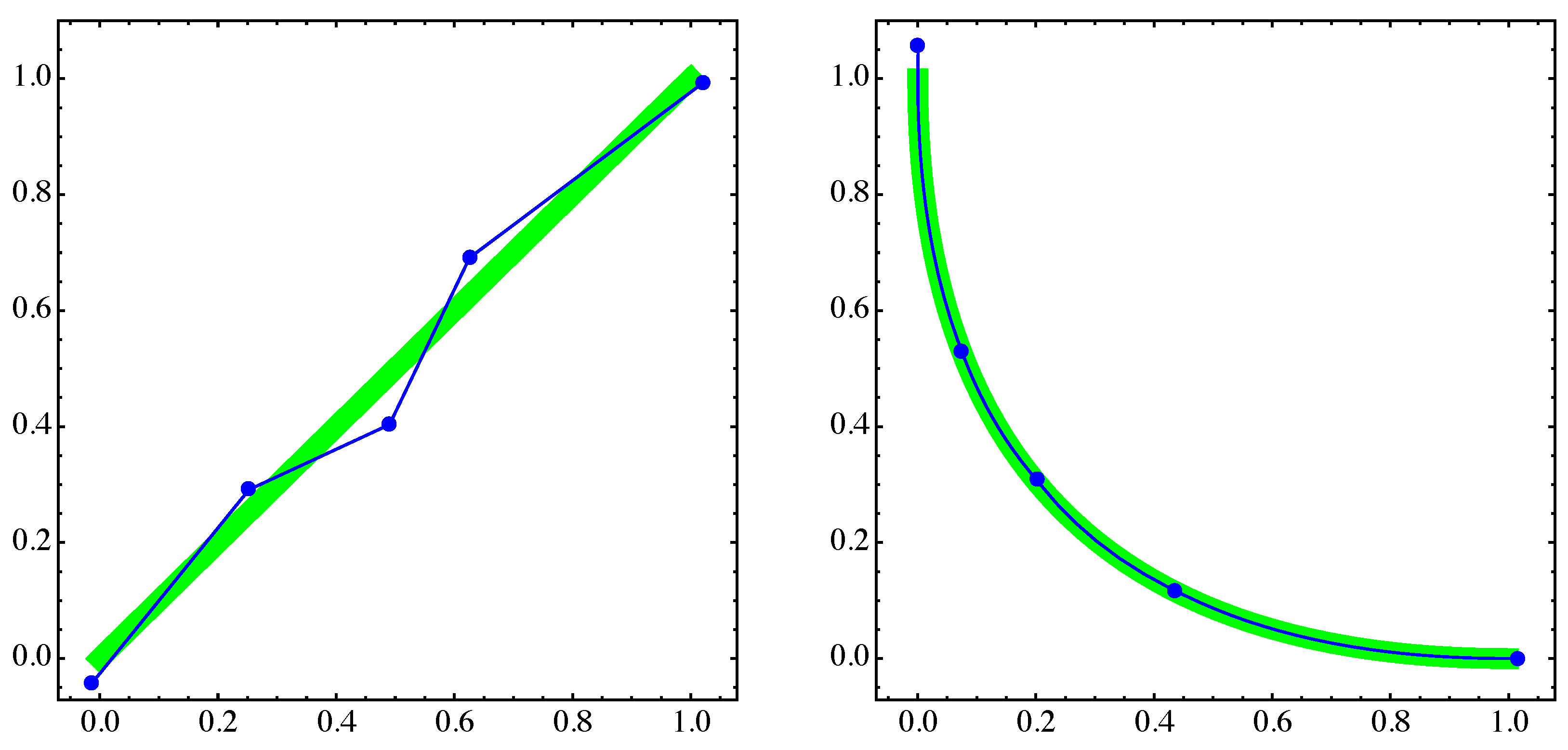
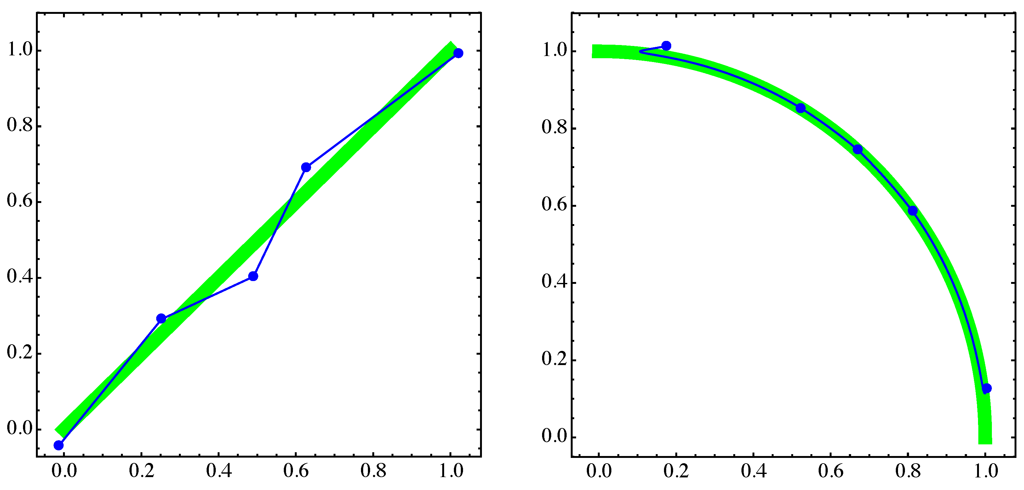
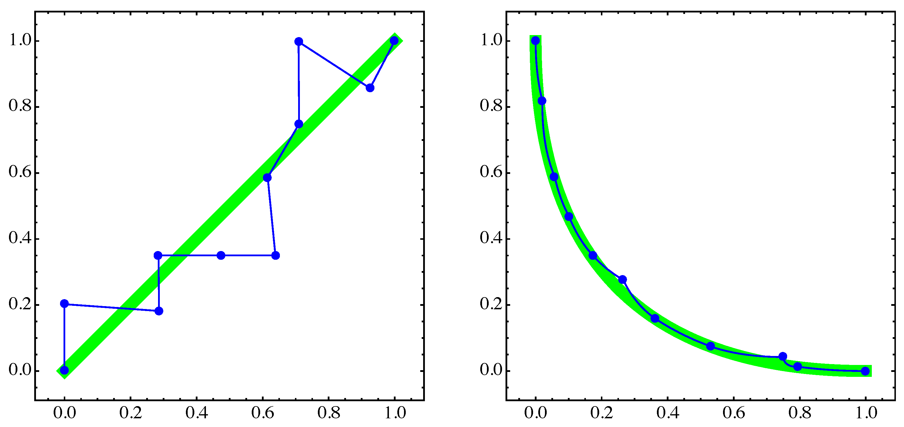
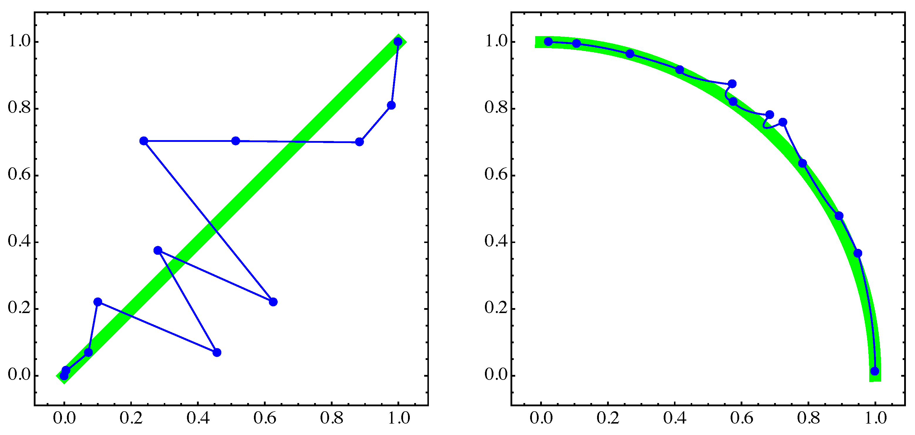
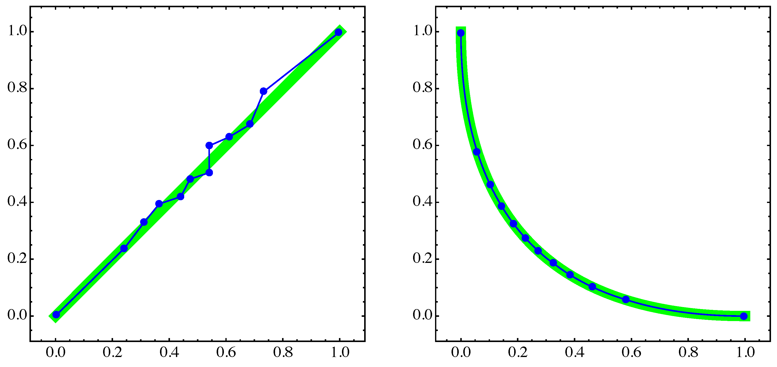
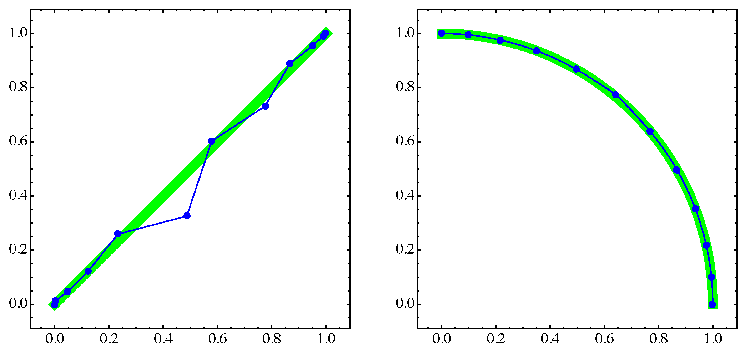
4. Numerical Examples

In this section, we demonstrate the applicability and usefulness of the new distance measure on two examples.

4.1. General Example

As a first example we consider the following sets within the Euclidean plane ${\mathbb{R}}^2$: the first set, A, is a line segment connecting two points $a=(-1,0)$ and $b=(1,0)$, i.e.,

$$A=\overline{ab}.$$

(10)

Next, for some given $\delta >0$ and any fixed value of $\epsilon >0$ we consider sets $B_{\delta }$ defined as the union of line segments

$$B_{\delta }=\overline{c{d}_{\delta }}\cup \overline{e_{\delta }{f}_{\delta }}\cup \overline{g_{\delta }h},$$

(11)

where $c=(-1,\epsilon )$, $d_{\delta }=(-\delta ,\epsilon )$, $e_{\delta }=(-\delta ,1)$, $f_{\delta }=(\delta ,1)$, $g_{\delta }=(\delta ,\epsilon )$, and $h=(1,\epsilon )$ are the segment end-points in ${\mathbb{R}}^2$. Hereby, a set $B_{\delta }$ can be seen as a certain approximation of A, where the segment $\overline{e_{\delta }{f}_{\delta }}$ can be considered to be the outlier in the approximation.

Figure 4 shows the sets A and $B_{\delta }$ for the values $\delta \in \{0.05,0.10,0.20,0.40\}$ and $\epsilon =0.10$. Apparently, for smaller $\delta$, the outlier region gets smaller, and hence, the approximation $B_{\delta }$ of A gets “better”. This is reflected by the values of the $(p,q)$-distance in

Table 1. ${\Delta }_{p,q}$ values for A and $B_{\delta }$ in (10) and (11), for different values of p, q, and $\delta$, with fixed $\epsilon =0.10$.

p	q	${\mathbf{\Delta }}_{\mathit{pq}}(\mathit{A},{\mathit{B}}_{0.05})$	${\mathbf{\Delta }}_{\mathit{pq}}(\mathit{A},{\mathit{B}}_{0.10})$	${\mathbf{\Delta }}_{\mathit{pq}}(\mathit{A},{\mathit{B}}_{0.20})$	${\mathbf{\Delta }}_{\mathit{pq}}(\mathit{A},{\mathit{B}}_{0.40})$
1	1	$0.7149$	$0.7464$	$0.8091$	$0.9324$
1	$-1$	$0.4105$	$0.4506$	$0.5311$	$0.6945$
1	$-100$	$0.1503$	$0.1961$	$0.2878$	$0.4711$
1	$-200$	$0.1479$	$0.1934$	$0.2844$	$0.4663$
1	$-10,000$	$0.1451$	$0.1901$	$0.2802$	$0.4602$

.

On the other hand, if choosing the classical Hausdorff distance, all values of $d_H(A,B_{\delta })$ are equal to 1, regardless of the choice of $\delta >0$. Hence, the $(p,q)$-distance is more appropriate in this example to identify “better” approximations.

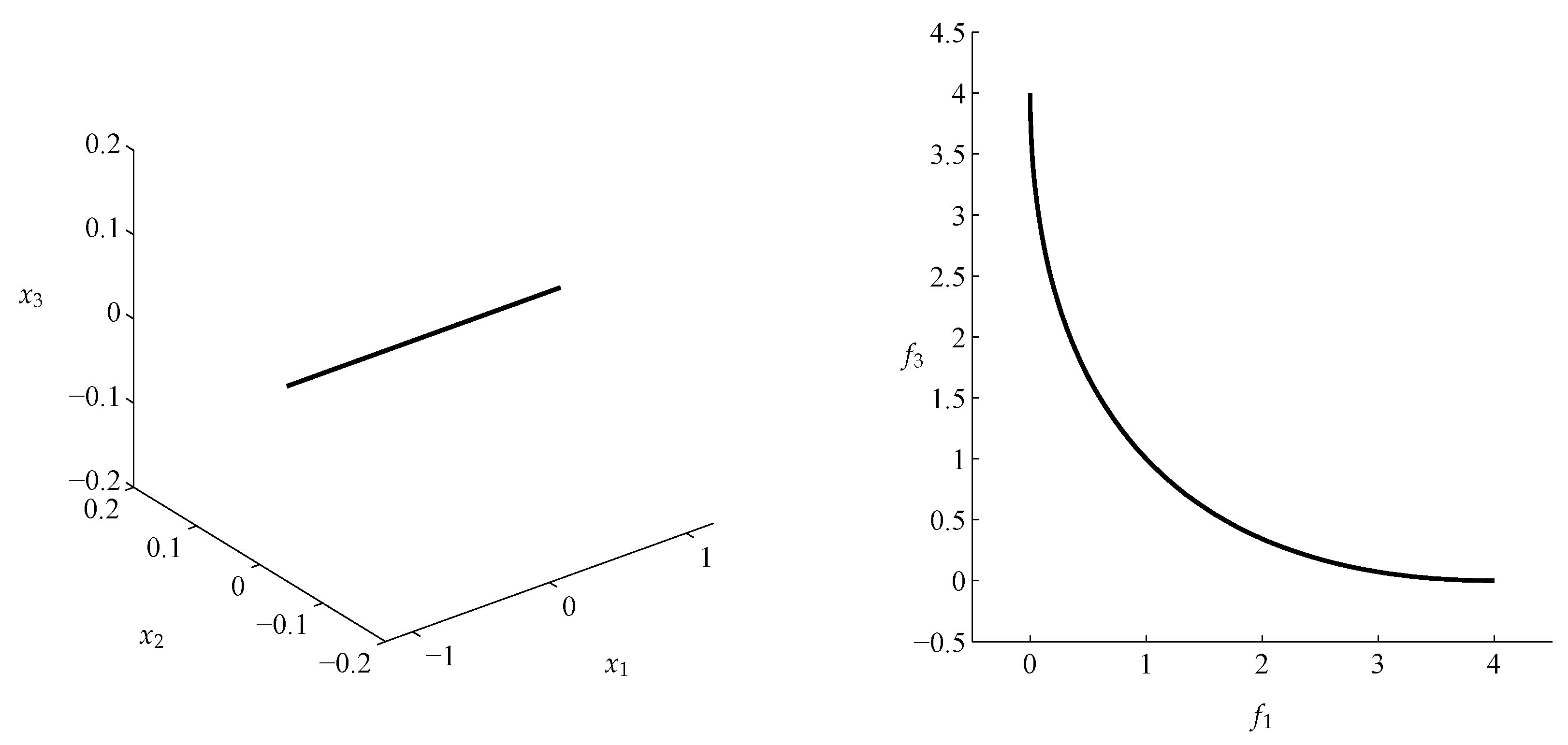
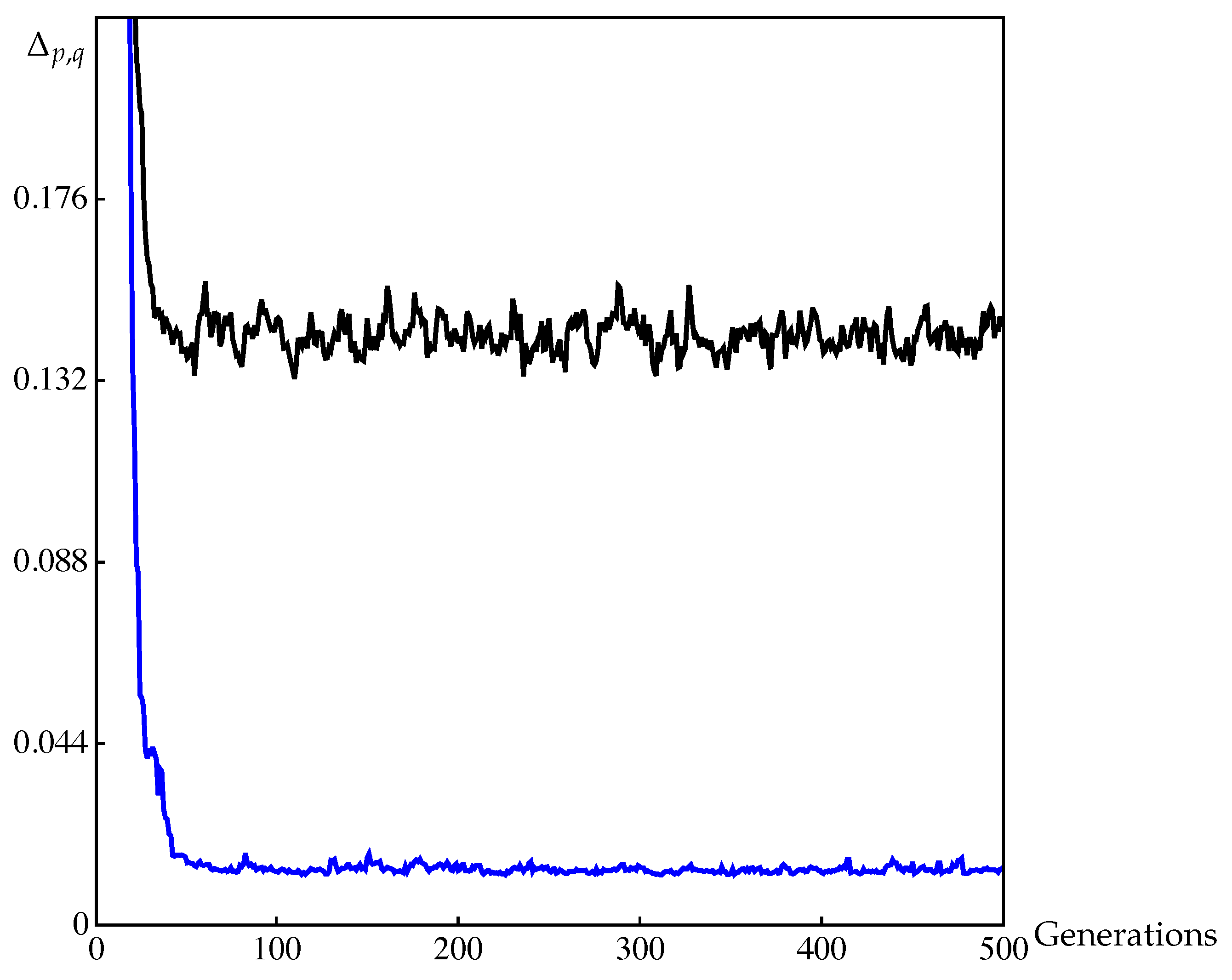
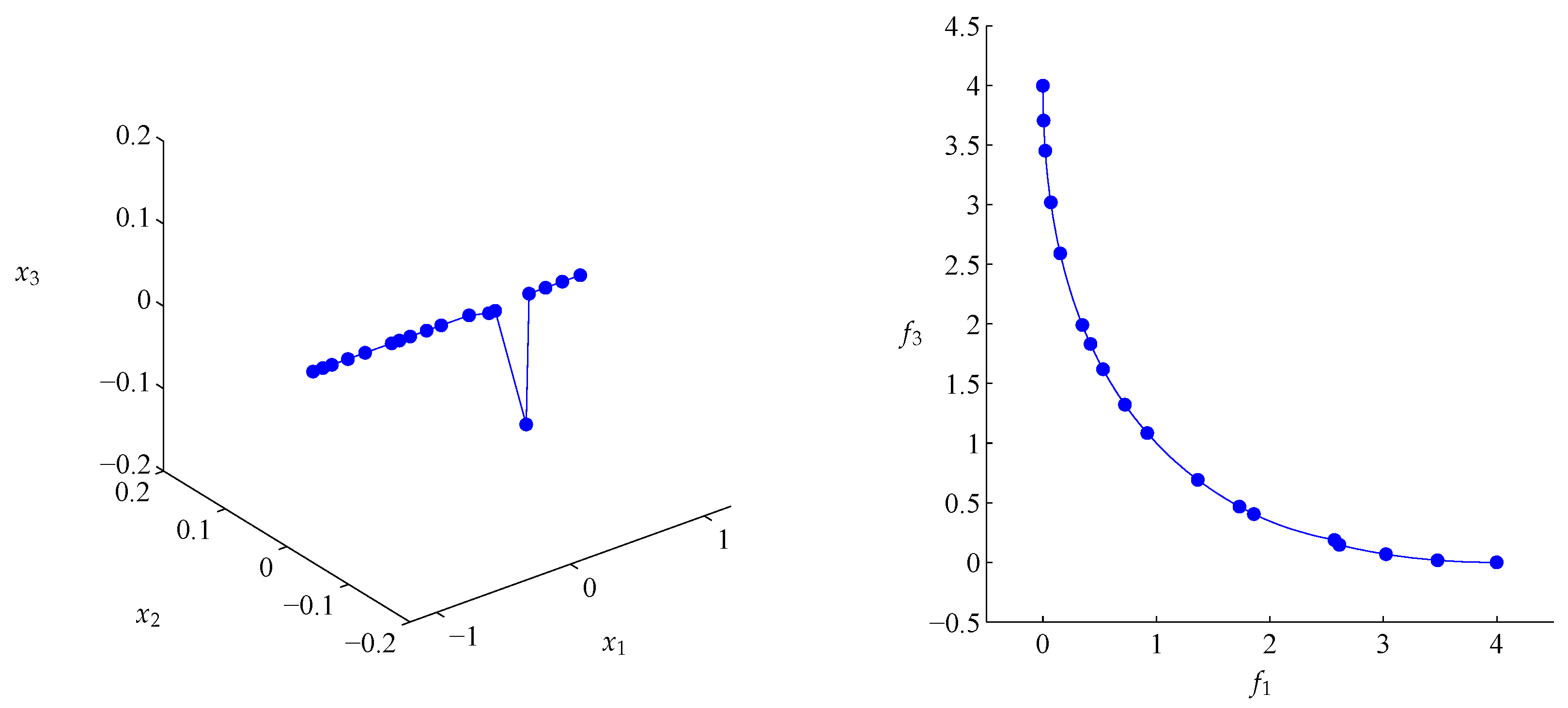
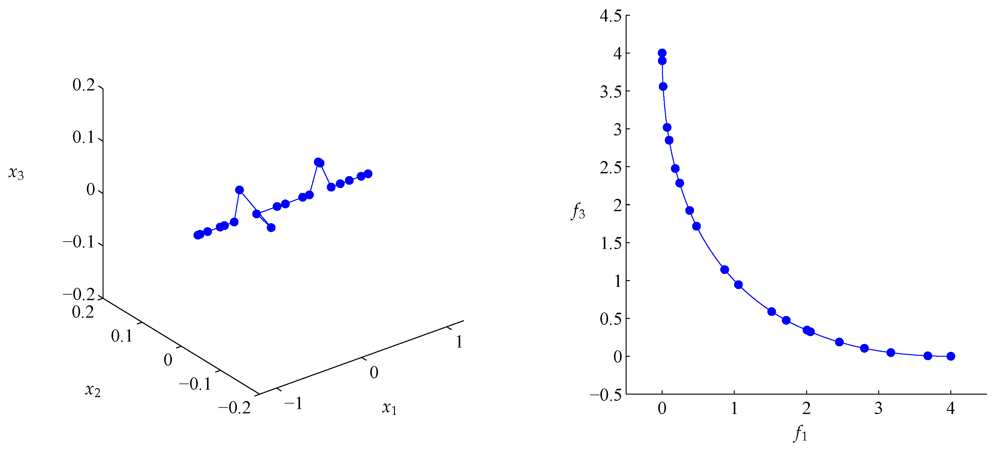
4.2. Approximation of Pareto Sets/Fronts

As a second example we consider the approximation of the Pareto set and front of a given MOP. For this, we define the following bi-objective problem that is known as the Lamé super-sphere function [32]:

$$\underset{x}{\min }F:{\mathbb{R}}^n\to {\mathbb{R}}^2,$$

(12)

where $F\left(x\right)=(f_1\left(x\right),f_2\left(x\right))$ is given by

$$f_1\left(x\right)={\left(\frac{1}{n}\sum _{i=1}^n{x}_i^2\right)}^{\frac{\gamma }{2}}\mathrm{and}{f}_2\left(x\right)={\left(\frac{1}{n}\sum _{i=1}^n{(x_i-1)}^2\right)}^{\frac{\gamma }{2}}$$

for $x\in {\mathbb{R}}^n$ and $\gamma \in \mathbb{R}$. Figure 5 and Figure 6 show the Pareto sets and fronts for the special cases $n=2$ with $\gamma =2$ and $\gamma =1/2$, respectively.

For the first step, we consider a simple hypothetical example to illustrate the concept of continuous archives in the context of evolutionary multi-objective optimization. For these, assume we are given the discrete archive $A=\{x_1,\dots ,x_5\}\subset {\mathbb{R}}^2$, where

$$\begin{array}{c}{x}_1=(-0.0129,-0.0421),x_2=(0.2525,0.2912),x_3=(0.4903,0.4035),\\ x_4=(0.6258,0.6912),x_5=(1.0212,0.9930).\end{array}$$

The set A is hence consisting of only five candidate solutions. Analogously, the image $F\left(A\right)$ of A can be considered as an approximation of the Pareto front that consists as well of five candidate solutions. Now, in order to improve the quality of the approximation, instead of A one can consider the polygon that is defined by the elements of A, namely

$$B:=\overline{x_1{x}_2}\cup \cdots \cup \overline{x_4{x}_5}.$$

(13)

In what follows, we will call this polygon the continuous archive. The approximations A, B, $F\left(A\right)$, and $F\left(B\right)$ can be seen in the Figure 7 and Figure 8. By visual inspection, the approximation qualities increase significantly when using the linear interpolation, in particular in objective space. This is reflected by the $(p,q)$-distances which are shown in

Table 2. ${\Delta }_{p,q}$ values for the Pareto set/front approximations for MOP (12).

	p	q	Decision Space		Objective Space
			Finite Archive	Continuous Archive	Finite Archive	Continuous Archive
$\gamma =2$	1	1	$0.5314$	$0.4841$	$0.4369$	$0.3943$
	1	$-1$	$0.2732$	$0.1750$	$0.2095$	$0.0945$
	1	$-100$	$0.1140$	$0.0213$	$0.0893$	$0.0018$
	1	$-200$	$0.1131$	$0.0208$	$0.0886$	$0.0017$
	1	$-10,000$	$0.1122$	$0.0202$	$0.0879$	$0.0017$
$\gamma =12$	1	1	$0.5314$	$0.4841$	$0.5629$	$0.5024$
	1	$-1$	$0.2732$	$0.1750$	$0.2807$	$0.1072$
	1	$-100$	$0.1140$	$0.0213$	$0.1202$	$0.0015$
	1	$-200$	$0.1131$	$0.0208$	$0.1192$	$0.0015$
	1	$-10,000$	$0.1122$	$0.0202$	$0.1183$	$0.0014$

where we can find the following general behavior: first, the distances within decision and objective spaces, decreases from finite to continuous archives, and this phenomena is stronger in the objective space; and second, following the result of Theorem 4, the distances decreases as q decreases.

In a next step, we consider discrete and continuous archives resulting from two of the most famous EMO algorithms: NSGA-II [44] and MOEA/D [45], see

Table 3. Parameter setting for NSGA-II and MOEA/D.

Algorithm	Parameter	Value
NSGA-II	Population size	12
	Number of generations	500
	Crossover probability	0.8
	Mutation probability	$1/n$
	Distribution index for crossover	20
	Distribution index for mutation	20
MOEA/D	Population size	12
	# weight vectors	12
	Number of generations	500
	Crossover probability	1
	Mutation probability	$1/n$
	Distribution index for crossover	30
	Distribution index for mutation	20
	Aggregation function	Tchebycheff
	Neighborhood size	3

for the parameter setting of these algorithms. To this end, we first consider the result of NSGA-II with a population size of 12 after 500 generations, see Figure 9 and Figure 10 and

Table 4. ${\Delta }_{p,q}$ values for the Pareto front approximations for MOP (12) using the NSGA-II archives and with $p=1$, $q=-10$.

Generation	$\mathit{\gamma }=1/2$		$\mathit{\gamma }=2$
	Finite Archive	Continuous Archive	Finite Archive	Continuous Archive
50	$0.0439$	$0.0147$	$0.0696$	$0.0160$
100	$0.0498$	$0.0109$	$0.0540$	$0.0102$
200	$0.0613$	$0.0118$	$0.0716$	$0.0207$
250	$0.0651$	$0.0265$	$0.0572$	$0.0061$
400	$0.0602$	$0.0102$	$0.0723$	$0.0276$
450	$0.0630$	$0.0154$	$0.0584$	$0.0088$
460	$0.0612$	$0.0154$	$0.0658$	$0.0098$
470	$0.0523$	$0.0102$	$0.0566$	$0.0083$
480	$0.0754$	$0.0269$	$0.0684$	$0.0241$
490	$0.0510$	$0.0091$	$0.0584$	$0.0118$
500	$0.0722$	$0.0097$	$0.0560$	$0.0103$

for the numerical results. Finally, we consider the MOEA/D generational algorithm to get 500 finite archives of 12 elements each, see Figure 11 and Figure 12 and

Table 5. ${\Delta }_{p,q}$ values for the Pareto front approximations for MOP (12) using the MOEA/D archives and with $p=1$, $q=-10$.

Generation	$\mathit{\gamma }=1/2$		$\mathit{\gamma }=2$
	Finite Archive	Continuous Archive	Finite Archive	Continuous Archive
50	$0.0610$	$0.0171$	$0.0648$	$0.0119$
100	$0.0519$	$0.0051$	$0.1093$	$0.0016$
200	$0.0536$	$0.0037$	$0.0781$	$0.0009$
250	$0.0522$	$0.0037$	$0.0790$	$0.0008$
400	$0.0511$	$0.0017$	$0.0784$	$0.0009$
450	$0.0511$	$0.0017$	$0.0784$	$0.0009$
460	$0.0509$	$0.0012$	$0.0784$	$0.0009$
470	$0.0509$	$0.0012$	$0.0784$	$0.0009$
480	$0.0509$	$0.0010$	$0.0783$	$0.0009$
490	$0.0509$	$0.0010$	$0.0783$	$0.0009$
500	$0.0509$	$0.0010$	$0.0783$	$0.0009$

for the numerical results.

For both EMO algorithms, it can be observed that the indicator values for the continuous archives are significantly better than for the respective discrete archives. Next, note that the ${\Delta }_{p,q}$ values oscillate for NSGA-II which is a typical behavior for this dominance-based algorithm. These oscillations, however, are less distinct for the continuous archives.

To further investigate the last statement, we consider finally the convex bi-objective problem $f_1,f_2:{\mathbb{R}}^3\to \mathbb{R}$, where $x=(x_1,x_2,x_3)$ and

$$\begin{array}{cc}\hfill f_1\left(x\right)& ={(x_1+1)}^2+x_2^2+x_3^2\hfill \\ \hfill f_2\left(x\right)& ={(x_1-1)}^2+x_2^2+x_3^2.\hfill \end{array}$$

(14)

The Pareto set of MOP (14) is the line segment connecting the points $(0,0,0)$ and $(1,0,0)$, and the Pareto front is as shown in Figure 13.

Figure 14 and

Table 6. ${\Delta }_{p,q}$ values for the discrete and continuous archives of NSGA-II for MOP (14). The results are averaged over 20 independent runs.

Generation	Continuous Archive	Finite Archive
20	$0.1333$	$0.2401$
40	$0.0176$	$0.1451$
60	$0.0090$	$0.1561$
80	$0.0088$	$0.1355$
100	$0.0065$	$0.1472$
120	$0.0074$	$0.1412$
140	$0.0081$	$0.1395$
160	$0.0075$	$0.1549$
180	$0.0092$	$0.1468$
200	$0.0074$	$0.1429$
220	$0.0066$	$0.1408$
240	$0.0075$	$0.1397$
260	$0.0066$	$0.1460$
280	$0.0074$	$0.1439$
300	$0.0084$	$0.1421$
320	$0.0070$	$0.1352$
340	$0.0070$	$0.1373$
360	$0.0081$	$0.1454$
380	$0.0079$	$0.1413$
400	$0.0066$	$0.1388$
420	$0.0063$	$0.1400$
440	$0.0097$	$0.1384$
460	$0.0067$	$0.1418$
480	$0.0067$	$0.1421$
500	$0.0076$	$0.1426$

show the ${\Delta }_{p,q}$ values for both the discrete and continuous archives obtained by NSGA-II using a population size of 20. As it can be seen, again the continuous archives achieve much better indicator values, and the amplitudes of the oscillations are significantly smaller compared to the discrete archives. This is confirmed by Figure 15, Figure 16 and Figure 17 that show the results of the discrete and continuous archives after 300, 400, and 500 generations, respectively. As it can be seen, NSGA-II is able to compute solutions along the Pareto front, however, with varying distribution along this set (In fact, it is known that there is no “limit archive” for NSGA-II since this algorithm is not indicator-based). In turn, for each of the results of NSGA-II, all of the continuous archives represent—at least by visual inspection—perfect approximations of the Pareto front, which is reflected by the good ${\Delta }_{p,q}$ values.

Concluding, the results presented in this section strongly indicate the convenience of the new indicator that is able to assess the performance of continuous archives. Though in principle also other indicators can be extended to continuous sets, this has not been done so far, and this is not a straightforward task. Hence, no comparisons to other indicators can be considered here. The presented results further indicate the benefit of the use of continuous archives instead of discrete ones that are being used classically. This would, among others, allow for the usage of smaller population sizes which would in turn allow to reduce the computational burden of the evolutionary algorithms (note that the time complexity for all MOEAs in each generation is quadratic in the population size). The verification of this statement, however, is left for future work as this goes beyond the scope of this study.

5. Conclusions and Future Work

In this work, we have proposed extensions of the existing ${\mathrm{GD}}_{p,q}$ and ${\Delta }_{p,q}$ performance indicators that allow to compute the distance between two general measurable sets. In particular, this is a natural setting in multi-objective optimization because the solution of such a problem typically forms a set of certain dimension (and is thus not given by finitely many points). We have shown that the extended indicators keep the nice metric properties from its finite-version predecessors (see [14,26]). Moreover, for ${\mathrm{GD}}_{p,q}$, sufficient conditions have been provided ensuring that certain compliance to Pareto optimality of this indicator can be guaranteed. Further study is needed to determine the precise relation between these conditions and other ones appearing in the literature.

We have demonstrated the applicability and usefulness of the novel indicator on examples related to evolutionary multi-objective optimization.

As part of future work, we intend to further investigate the use of ${\Delta }_{p,q}$ within evolutionary multi-objective optimization. For instance, it might be interesting to integrate this performance indicator within an evolutionary multi-objective optimization algorithm as it was done, e.g., in [46] for its predecessor ${\Delta }_p$. Although it is clear that the individual roles of p and q are related with the convexity of the metric neighborhoods of point and sets, further research is needed to elucidate more precisely useful ways to take advantage of their joint behavior in concrete situations. Additionally, to understand the behavior of ${\Delta }_{p,q}$ in relation to Pareto compliance and to complete the partial results that have been established in Section 3.4 for ${\mathrm{GD}}_{p,q}$, consideration should be given to the inverted generational indicator ${\mathrm{IGD}}_{p,q}$. Finally, one interesting aspect is to see if the indicator can be used as a proximity measure in other research fields.

References

- Heinonen, J. Lectures on Analysis on Metric Spaces; Springer: New York, NY, USA, 2001. [Google Scholar]
- Huttenlocher, D.P.; Klanderman, G.A.; Rucklidge, W.A. Comparing Images Using the Hausdorff Distance. IEEE Trans. Pattern Anal. Mach. Intell. 1993, 15, 850–863. [Google Scholar] [CrossRef]
- Yi, X.; Camps, O.I. Line-Based Recognition Using A Multidimensional Hausdorff Distance. IEEE Trans. Pattern Anal. Mach. Intell. 1999, 21, 901–916. [Google Scholar]
- De Carvalho, F.; de Souza, R.; Chavent, M.; Lechevallier, Y. Adaptive Hausdorff distances and dynamic clustering of symbolic interval data. Pattern Recognit. Lett. 2006, 27, 167–179. [Google Scholar] [CrossRef]
- Dellnitz, M.; Hohmann, A. A subdivision algorithm for the computation of unstable manifolds and global attractors. Numerische Mathematik 1997, 75, 293–317. [Google Scholar] [CrossRef]
- Aulbach, B.; Rasmussen, M.; Siegmund, S. Approximation of attractors of nonautonomous dynamical systems. Discret. Contin. Dyn. Syst. Ser. B 2005, 5, 215–238. [Google Scholar]
- Emmerich, M.; Deutz, A.H. Test Problems Based on Lamé Superspheres. In Proceedings of the 4th International Conference on Evolutionary Multi-criterion Optimization, Matsushima, Japan, 5–8 March 2007; Springer: Berlin/Heidelberg, Germany, 2007; pp. 922–936. [Google Scholar]
- Falconer, K. Fractal Geometry: Mathematical Foundations and Applications, 2nd ed.; John Wiley & Sons, Inc.: Hoboken, NJ, USA, 2003. [Google Scholar]
- Schütze, O. Set Oriented Methods for Global Optimization. Ph.D. Thesis, University of Paderborn, Paderborn, Germany, 2004. [Google Scholar]
- Dellnitz, M.; Schütze, O.; Hestermeyer, T. Covering Pareto Sets by Multilevel Subdivision Techniques. J. Optim. Theory Appl. 2005, 124, 113–155. [Google Scholar] [CrossRef]
- Padberg, K. Numerical Analysis of Transport in Dynamical Systems. Ph.D. Thesis, University of Paderborn, Paderborn, Germany, 2005. [Google Scholar]
- Schütze, O.; Coello Coello, C.A.; Mostaghim, S.; Talbi, E.G.; Dellnitz, M. Hybridizing Evolutionary Strategies with Continuation Methods for Solving Multi-Objective Problems. Eng. Optim. 2008, 40, 383–402. [Google Scholar] [CrossRef]
- Schütze, O.; Laumanns, M.; Coello Coello, C.A.; Dellnitz, M.; Talbi, E.G. Convergence of Stochastic Search Algorithms to Finite Size Pareto Set Approximations. J. Glob. Optim. 2008, 41, 559–577. [Google Scholar] [CrossRef]
- Schütze, O.; Esquivel, X.; Lara, A.; Coello Coello, C.A. Using the averaged Hausdorff distance as a performance measure in evolutionary multiobjective optimization. IEEE Trans. Evol. Comput. 2012, 16, 504–522. [Google Scholar] [CrossRef]
- Hernández, C.; Naranjani, Y.; Sardahi, Y.; Liang, W.; Schütze, O.; Sun, J.Q. Simple Cell Mapping Method for Multi-objective Optimal Feedback Control Design. Int. J. Dyn. Control 2013, 1, 231–238. [Google Scholar] [CrossRef]
- Siwel, J.; Yew-Soon, O.; Jie, Z.; Liang, F. Consistencies and contradictions of performance metrics in multiobjective optimization. IEEE Trans. Evol. Comput. 2014, 44, 2329–2404. [Google Scholar]
- Sun, J.Q.; Xiong, F.R.; Schütze, O.; Hernández, C. Cell Mapping Methods—Algorithmic Approaches and Applications; Springer: Singapore, 2019. [Google Scholar]
- Jahn, J. Multiobjective search algorithm with subdivision technique. Comput. Optim. Appl. 2006, 35, 161–175. [Google Scholar] [CrossRef]
- Schütze, O.; Vasile, M.; Junge, O.; Dellnitz, M.; Izzo, D. Designing optimal low thrust gravity assist trajectories using space pruning and a multi-objective approach. Eng. Optim. 2009, 41, 155–181. [Google Scholar] [CrossRef]
- Deb, K. Multi-Objective Optimization Using Evolutionary Algorithms; John Wiley & Sons: Chichester, UK, 2001. [Google Scholar]
- Beume, N.; Naujoks, B.; Emmerich, M. SMS-EMOA: Multiobjective selection based on dominated hypervolume. Eur. J. Oper. Res. 2007, 181, 1653–1669. [Google Scholar] [CrossRef]
- Garg, H. Solving structural engineering design optimization problems using an artificial bee colony algorithm. J. Ind. Manag. Optim. 2014, 10, 777–794. [Google Scholar] [CrossRef]
- Garg, H. A hybrid PSO-GA algorithm for constrained optimization problems. Appl. Math. Comput. 2016, 274, 292–305. [Google Scholar] [CrossRef]
- Zapotecas-Martínez, S.; López-Jaimes, A.; García-Nájera, A. LIBEA: A Lebesgue Indicator-Based Evolutionary Algorithm for Multi-objective Optimization. Swarm Evolut. Comput. 2018. [Google Scholar] [CrossRef]
- Hartikainen, M.; Miettinen, K.; Wiecek, M. PAINT: Pareto front interpolation for nonlinear multiobjective optimization. Comput. Optim. Appl. 2012, 52, 845–867. [Google Scholar] [CrossRef]
- Vargas, A.; Bogoya, J.M. A generalization of the averaged Hausdorff distance. Computación y Sistemas 2018, 22, 331–345. [Google Scholar] [CrossRef]
- Tao, T. An Introduction to Measure Theory (Graduate Studies in Mathematics); American Mathematical Society: Providence, RI, USA, 2011. [Google Scholar]
- Jones, F. Lebesgue Integration on Euclidean Space; Jones and Bartlett Publishers: Boston, MA, USA, 2001. [Google Scholar]
- Hardy, G.H.; Littlewood, J.E.; Pólya, G. Inequalities, 2nd ed.; Cambridge University Press: Cambridge, UK, 1952. [Google Scholar]
- Bullen, P.S. Handbook of Means and Their Inequalities; Kluwer Academic Publishers Group: Dordrecht, The Netherlands, 2003. [Google Scholar]
- Pareto, V. Manual of Political Economy; The Macmillan Press: London, UK, 1971. [Google Scholar]
- Hillermeier, C. Nonlinear Multiobjective Optimization: A Generalized Homotopy Approach; Springer Science & Business Media: Berlin, Germany, 2001. [Google Scholar]
- Zitzler, E.; Thiele, L. Multiobjective evolutionary algorithms: A comparative case study and the strength Pareto approach. IEEE Trans. Evol. Comput. 1999, 3, 257–271. [Google Scholar] [CrossRef]
- Brockhoff, D.; Wagner, T.; Trautmann, H. On the Properties of the R2 Indicator. In Proceedings of the 14th Annual Conference on Genetic and Evolutionary Computation, Philadelphia, PA, USA, 7–11 July 2012; ACM: New York, NY, USA, 2012; pp. 465–472. [Google Scholar]
- Ishibuchi, H.; Masuda, H.; Nojima, Y. A Study on Performance Evaluation Ability of a Modified Inverted Generational Distance Indicator. In Proceedings of the 2015 Annual Conference on Genetic and Evolutionary Computation, Madrid, Spain, 11–15 July 2015; ACM: New York, NY, USA, 2015; pp. 695–702. [Google Scholar]
- Dilettoso, E.; Rizzo, S.A.; Salerno, N. A Weakly Pareto Compliant Quality Indicator. Math. Comput. Appl. 2017, 22, 25. [Google Scholar]
- Garg, H.; Kumar, K. Distance measures for connection number sets based on set pair analysis and its applications to decision-making process. Appl. Intell. 2018, 48, 1–14. [Google Scholar] [CrossRef]
- Singh, S.; Garg, H. Distance measures between type-2 intuitionistic fuzzy sets and their application to multicriteria decision-making process. Appl. Intell. 2017, 46, 788–799. [Google Scholar] [CrossRef]
- Van Veldhuizen, D.A.; Lamont, G.B. Multiobjective evolutionary algorithm test suites. In Proceedings of the 1999 ACM Symposium on Applied Computing, San Antonio, TX, USA, 28 February–2 March 1999; ACM: New York, NY, USA, 1999; pp. 351–357. [Google Scholar]
- Coello Coello, C.A.; Cruz Cortés, N. Solving Multiobjective Optimization Problems using an Artificial Immune System. Genet. Program. Evolvable Mach. 2005, 6, 163–190. [Google Scholar] [CrossRef]
- Rudolph, G.; Schütze, O.; Grimme, C.; Domínguez-Medina, C.; Trautmann, H. Optimal averaged Hausdorff archives for bi-objective problems: Theoretical and numerical results. Comput. Optim. Appl. 2016, 64, 589–618. [Google Scholar] [CrossRef]
- Zitzler, E.; Thiele, L.; Laumanns, M.; Fonseca, C.M.; da Fonseca, V.G. Performance assessment of multiobjective optimizers: An analysis and review. IEEE Trans. Evol. Comput. 2003, 7, 117–132. [Google Scholar] [CrossRef]
- Witkowski, A. A new proof of the monotonicity property of power means. JIPAM. J. Inequal. Pure Appl. Math. 2004, 5, 73. [Google Scholar]
- Deb, K.; Pratap, A.; Agarwal, S.; Meyarivan, T. A fast and elitist multiobjective genetic algorithm: NSGA-II. IEEE Trans. Evol. Comput. 2002, 6, 182–197. [Google Scholar] [CrossRef]
- Zhang, Q.; Li, H. MOEA/D: A Multiobjective Evolutionary Algorithm Based on Decomposition. IEEE Trans. Evol. Comput. 2007, 11, 712–731. [Google Scholar] [CrossRef]
- Schütze, O.; Domínguez-Medina, C.; Cruz-Cortés, N.; de la Fraga, L.G.; Sun, J.Q.; Toscano, G.; Landa, R. A scalar optimization approach for averaged Hausdorff approximations of the Pareto front. Eng. Optim. 2016, 48, 1593–1617. [Google Scholar] [CrossRef]