Automated Image Analysis for Retention Determination in Centrifugal Partition Chromatography

Abstract

In Centrifugal Partition Chromatography, two immiscible liquids are used as mobile and stationary phases. During operation, bleeding of the stationary phase cannot be eliminated completely. For optimal separation performance, however, it is crucial to maintain sufficient amounts of stationary phase in the system, which is quantitatively measured by the retention value. With an online measurement of that retention value, it is possible to make predictions about the separation performance of the system. Therefore, an image processing algorithm was developed in this study, allowing quick and effortless online evaluation of retention by image analysis. Finally, the results were compared with proven analysis methods to evaluate the measurements’ validity. With the help of the new algorithm, it was possible to improve the number of pictures analyzed per time and the precision compared to the previously used technique.

1. Introduction

Countercurrent Chromatography can be differentiated into two different technical concepts: instruments containing at least one coil that rotates in a planetary trajectory (hydrodynamic CCC) and apparatuses consisting of rotor discs with embedded cells rotating around a single axis (hydrostatic CCC). The latter is also known as Centrifugal Partition Chromatography (CPC) and is particularly interesting for industrial applications due to its comparatively straightforward technical implementation. Although the term Countercurrent Chromatography (CCC) suggests otherwise, one liquid phase is immobilized in such an apparatus being the stationary phase, and a second liquid phase is actively pumped as a mobile phase. Thus, when compared to conventional liquid chromatography, the solid stationary phase is replaced by a second liquid immiscible with the mobile phase that is kept in the CPC apparatus by centrifugal force [1].

The use of two liquid phases has several advantages over a solid-liquid system, for example, high loading capacities and total recovery since no irreversible adsorption is possible in a liquid-liquid system. In terms of costs per capacity, liquid stationary phases are usually much less expensive than packed solids. Furthermore, the packing process of the solid material is no longer a source of error, and environmentally friendly solvents (e.g., Aqueous Two-Phase Systems) are available. At the same time, solvents are ideal for processing sensitive substances such as proteins [1,2,3]. Besides, there are further fields of application: In the context of Quantitative Structure–Activity Relationship (QSAR) analysis, CPC can be used to determine partition coefficients. With the help of these data sets, QSAR models can be implemented, allowing for the prediction of partition coefficients based on the molecular structure [4,5].

For initial start-up, the centrifugal chromatograph is filled with a stationary phase. The mobile phase is subsequently pumped into the rotor and is dispersed within the stationary phase at each chamber inlet. The mass transfer takes place in the resulting dispersion zone. A coalescence zone of the mobile phase is formed at each chamber outlet. Thus, in an ideal case, each CPC chamber acts as a mixer-settler unit known for extraction processes. In order to work as described, retention is a key parameter to ensure optimal separation performance. Until today, the determination of that crucial parameter requires manual work and time after each experimental CPC run. Therefore, quantitative online monitoring of the retention was hardly performable, and the total number of parameter sets being investigated according to their retention was severely limited [6]. With rapidly evolving image processing technology and the resulting potentials, the goals of the work reported here are, therefore, to reduce the duration of the evaluation on the one hand and to increase the accuracy on the other hand [7]. For this reason, a Matlab-based routine was developed and implemented, automating the analysis of raw data supplied by a high-speed camera [8]. Image processing algorithms were used to eliminate the need for manual editing, speeding up the determination of retention as well as removing the human error source from the process.

2. Theory

For the determination of retention in CPC, a visual inspection ensures precise raw data. Therefore, it is crucial to utilize transparent rotors. The combination of camera technology and sophisticated image analysis has already been used to obtain information about the flow regime present [9,10]. In this study, the determination of the retention value Sf* (Equation (1)) is of particular interest [6].

$$S{f}^{*}=\frac{V_{stat,c}+V_{stat,d}}{V_c}$$

(1)

The Sf* is calculated from the volume of stationary phase inside the chambers V_stat,c and ducts V_stat,d as well as the total volume of the chambers V_c and provides information on the amount of stationary phase remaining in each chamber during operation. The optimum range is between 0.25 ≤ Sf ≤ 0.75, with low Sf* values resulting in a chromatogram showing short retention times and closely spaced peaks. Identical components elute much later and with higher resolution at high Sf* values [1].

In order to determine Sf*, mobile phase flow has to be stopped temporarily. Next, a video of the resting liquid phases in the chambers and ducts can be recorded. It is a state of the art to process the raw data by hand [6]. For this purpose, a polygonal path is placed around a single chamber-duct combination. This procedure has to be repeated for each chamber, from which an Sf* shall be calculated. A manually marked polygonal path is shown in Figure 1 as an example, where the stationary phase occupies part of the chamber as well as part of the channel.

The number of white pixels within this area is then evaluated using the image processing tool ImageJ [11]. The actual Sf* is determined subsequently by calculating the ratio of bright pixels to the total number of pixels inside the chamber [6].

3. Materials and Methods

3.1. Retention: Raw Data Acquisition

3.1.1. Chemicals

For all experiments performed during this study, the Arizona N system was used [12]. It was prepared by adding equal volumes of ethyl acetate (purity = 99.9%), heptane (purity = 99.8%), methanol (purity = 99%), all purchased from VWR International (Radnor, PA, USA), and water purified by a MILLI-Q^® system (Millipak^® Express 40, Merck, Darmstadt, Germany). The aqueous phase was selectively dyed (Methylene blue, Merck KGaA, 20 mg/L).

3.1.2. Rotor Configuration and Manual Sf* Determination

A semi-transparent rotor was used in a modified CPC (Type: FCPC, Chromaton^® (Annonay, France), descending mode, 1000 rpm, 15 mL/min mobile phase flow) as it has already been described in the literature [5,6]. The manual retention evaluation method was executed as described in Section 2. The rotor consists of a single disk with 66 chambers and connecting channels embedded. In contrast to stacked rotor versions, which are used for actual separation tasks (stacked and interconnected individual discs ensure a higher number of theoretical stages), the rotor mentioned is suitable for visual fluid flow detection.

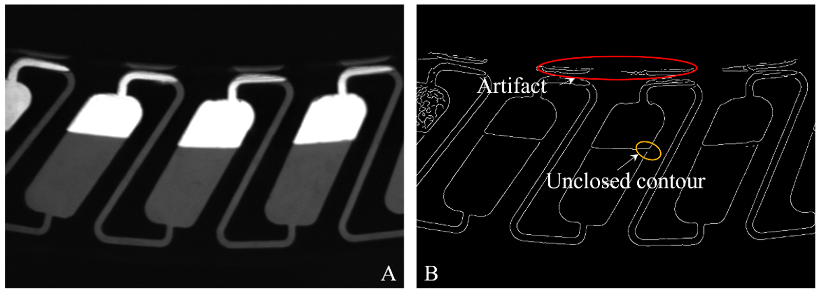
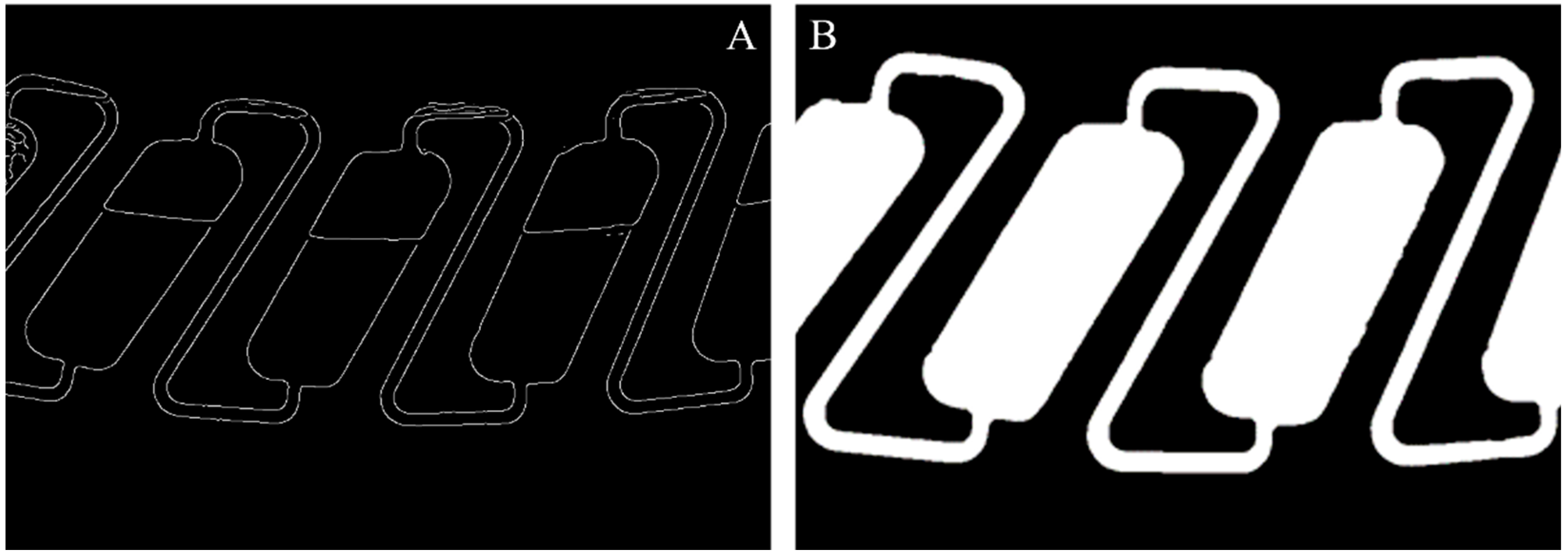
3.2. Newly Developed Image Processing Algorithm

The raw data for the new algorithm were still images extracted from the high-speed footage recorded at defined time intervals t_ext (Figure 2A). The edge detection algorithm “Canny” was then applied to the gray-scale images. It is based on the search for local maxima of the intensity gradient, where the latter is determined by smoothing the image with a Gaussian filter (Figure 2B) [13].

The binary image generated was examined for unclosed contours, according to Kovesi, and those gaps were filled [14]. For this purpose, a circular area with a radius of half the width of the gap to be closed (user-defined parameter) was created at the corner points of each edge segment. If two of these circles overlapped, they were reduced to a one-pixel-wide direct connection. On the other hand, the original edge was restored if there were no contact points. Besides the correction of unclosed contours, it was also necessary to eliminate artifacts in the binary image. These were caused by camera flash reflections in the viewing windows’ aluminum framing, which would interfere with further image processing.

In order to do so, a cutout of a ring-shaped mask was multiplied by the existing binary image (Figure 3A). This was possible because the data formats are compatible: multiplying a matrix with binary values to another matrix with the same data type gives the intersection of positive data points (pixels).

The areas enclosed by contours were then set to the binary value 1, which is why they appear white (Figure 3B). To calculate the retention value, Sf* (Equation (1)) was subdivided into a proportion assigned to the chambers (Sf*_c) and a proportion assigned to the ducts (Sf*_d), as the stationary phase occupies part of the chamber and part of the duct (Figure 1). Besides, the result was normalized to the corresponding number of chambers n_c and ducts n_d evaluated (Equation (2)).

$$S{f}_c^{*}=\frac{\frac{V_{stat,c}}{n_c}}{\frac{V_c}{n_c}} S{f}_d^{*}=\frac{\frac{V_{stat,d}}{n_d}}{\frac{V_c}{n_c}}$$

(2)

To determine the variables n_d, n_c, V_stat,c, V_stat,d, and V_c information from the unprocessed still image (Figure 2A) and the binary image (Figure 3B) was used. The volume of the chambers (V_c) and ducts were calculated by multiplying their depth in the direction of the rotation axis with their surface area. The surface area and the number of chambers and ducts (n_d, n_c) were determined by isolating the chambers through a sequence of erode and dilate commands (Figure 4A). Another binary image with exposed ducts was obtained analogously by subtracting the result obtained from the aforementioned binary image (Figure 4B). The unknown number of ducts and chambers and their surface area/volume were evaluated with this sequence of operations.

The fraction of stationary phase in the chambers and ducts was determined by using each chamber or duct isolated as a mask and multiplying it with the extracted non-binary still image. After that, the images obtained were binarized again (Figure 4C,D). The proportion of white pixels was evaluated and provided information about the remaining variables V_stat,c and V_stat,d. In this context, it was essential to consider which phase was colored and therefore appears dark in the video material. In the example presented in Figure 2, the heavy phase was dyed, and the centrifugal chromatograph was operated in descending mode. However, it is also possible to analyze in ascending mode or when the light phase is dyed (user parameters).

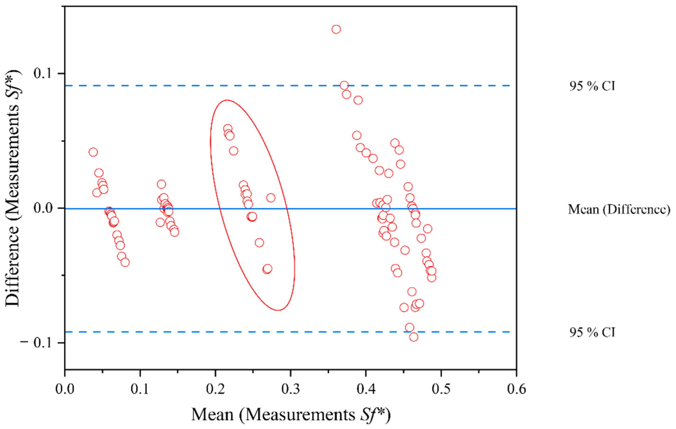
3.3. Method Comparison

For comparison of the manual and automated measurement methods, the Bland–Altman plot was utilized. [15] When a sample with i different data points is analyzed, two different methods give 2i measurement results. The data points can be plotted with the mean of the two methods on the abscissa and the respective difference on the ordinate, resulting in the Bland–Altman plot with i data points. Additional lines are often plotted for visual support, representing the 95% confidence interval. In combination, this information can be used to identify any differences (e.g., proportional bias) between the two measurement methods.

4. Results and Discussion

Benchmarking the Image Analysis Routine

The data set recorded according to Section 3.1.2 was analyzed by applying the following user parameters: descending mode, heavy phase dyed, t_ext = 0.5 s, resulting in 18 still images for each of the six videos recorded. For those images, a value for the retention of the stationary phase in the chambers, the ducts, and the chamber-duct combinations was determined using the procedure described in the previous section. The value for the chamber-duct-combination was re-evaluated via the manual image analysis described above, serving as a benchmark (Section 2). A mean retention value of 0.2921 was obtained for the manual method, and the evaluation via edge detection resulted in a mean value of 0.2916. That similarity between the mean values is a necessary but not yet a sufficient condition for the equivalence of both measurement methods. Considering the standard deviations of retention values for single inspection windows, a significant difference in precision is noticeable (Figure 5).

The mean retention value for the first inspection window is 0.0584 when measured with the automated method and 0.0611 using the manual method. However, the standard deviation differs tenfold, being 0.0027 with the automated and 0.0228 with the manual method. This trend is present for all inspection windows and indicates the superiority of the new image analysis routine developed.

A simple Pearson’s Correlation would not be sufficient to compare those paired data sets further. However, the Bland–Altman plot is appropriate for this purpose [15]. As mentioned, the same dataset (raw data available as Supplementary Materials) of still images was analyzed with two methods for direct method comparison. Furthermore, according to Bland and Altman, a graphical evaluation yields in the plot shown in Figure 6.

The relative difference of the retention values derived from the two measurement methods is plotted over the mean Sf*-value of both. It is noticeable that the variability of the evaluation methods for retention values in the range Sf* ≤ 0.3 is small (with values of +/− 0.06) and also lies within the 95% confidence interval (blue dashed lines) in all cases.

With higher mean Sf* values, the relative difference between the methods increases, whereby with Sf* values > 0.3, the 95 % confidence interval is exceeded in a few cases. Nevertheless, no significant systematic error can be identified, indicating an inconsistency in the measurement methods being compared. Considering Figure 5, the automated evaluation can be referred to as the new “gold standard” because of its significantly lower standard deviation. The angled cluster of data points for every inspection window (Figure 6, red ellipse marking the third inspection window as an example) is another indicator of the lower accuracy of the manual evaluation method. Such a pattern occurs for a collection of data points with a similar true value if one method’s precision is higher. For instance, if the manual method gives a value too low, while the automated method gives a value close to the true value, the mean value is shifted left, and the relative difference is shifted up (Section 3.3) and vice versa. However, if both methods show similar deviations from the true value, angled clusters like those in Figure 6 do not occur.

In summary, the average discrepancy between the methods is below 1%, which can be considered negligible. Besides, there is no proportional bias evident. It can be stated that the measurement methods compared in this section provide the same accuracy, with the automated method providing more precise data. Apart from precision, there are other criteria for comparing both techniques. The amount of time saved is an argument favoring automated edge detection. The effort for processing the data given (108 still images) is cut from several hours to just 55 s. Another important aspect is the exclusion of human error sources. While there is an observable wandering deviation with changing personnel using the manual method, the automated analysis ensures reproducible results. In addition, the automated evaluation provides the possibility for retention determination during operation.

5. Conclusions

Using fully automated image processing, we developed a new routine for analyzing retention inside a Centrifugal Partition Chromatograph. After comparison with the manual evaluation of the raw data with the help of a Bland–Altman plot, we demonstrated that both methods provide equivalently accurate results. The main advantages of automated evaluation, the lower standard deviation combined with significant time saving, allow for new process monitoring and control potentials. The determination of locally resolved retention values in the entire rotor during operation is now ready to be implemented, while the vast number of images is almost impossible to process manually. Identifying the current operating status of a centrifugal chromatograph is a huge step towards the implementation of those novel apparatuses in industry. Furthermore, the data can be used to control the operating parameters of the apparatus to prevent progressive flooding with the mobile phase (so-called bleeding), enabling long-term operability.

Of course, the rotor described is not particularly suitable for separation tasks. As mentioned, rotors in this context comprise more chambers to ensure sufficient separation performance. The rotor used in this study, which is observable with the camera technique, has a crucial function in understanding the influence of operating conditions and design parameters. After the interconnections are understood, the knowledge gained can be transferred to rotors consisting of several non-transparent disks. Compared with different approaches to measure the retention in Centrifugal Partition Chromatography (for example, phase separation at the device outlet and subsequent ratio determination of mobile and stationary phase), the innovative approach presented enables local resolution of bleeding within the rotor. Thus, the exact location of discharged stationary phase, and consequently, local hydrodynamic causes, can be identified. For instance, that is important when investigating the impact of sample injection. Because the sample contains at least one additional component compared to the mobile phase, it is not in equilibrium with the stationary phase. Therefore, it may initiate stationary sample loss, although the CPC was in stable operation before. In the next step, it is planned to analyze bleeding in a temporally as well as spatially resolved manner.

References

1. Berthod, A. Countercurrent Chromatography: The Support-Free Liquid Stationary Phase; Elsevier: Amsterdam, The Netherlands, 2002; ISBN 9780444507372. [Google Scholar]
2. Friesen, J.B.; McAlpine, J.B.; Chen, S.-N.; Pauli, G.F. Countercurrent Separation of Natural Products: An Update. J. Nat. Prod. 2015, 78, 1765–1796. [Google Scholar] [CrossRef] [Green Version]
3. Szekely, G.; Zhao, D. Sustainable Separation Engineering: Materials, Techniques and Process Development; John Wiley & Sons Ltd.: Hoboken, NJ, USA, 2022; ISBN 9781119740087. [Google Scholar]
4. Kukula-Koch, W.; Kruk-Słomka, M.; Stępnik, K.; Szalak, R.; Biała, G. The Evaluation of Pro-Cognitive and Antiamnestic Properties of Berberine and Magnoflorine Isolated from Barberry Species by Centrifugal Partition Chromatography (CPC), in Relation to QSAR Modelling. Int. J. Mol. Sci. 2017, 18, 2511. [Google Scholar] [CrossRef] [Green Version]
5. Marsden-Jones, S.C. The Application of Quantitative Structure Activity Relationship Models to the Method Development of Countercurrent Chromatography. Ph.D. Thesis, Brunel University, London, UK, 2015. [Google Scholar]
6. Fromme, A. Systematic Approach Towards Solvent System Selection for Ideal Fluid Dynamics in Centrifugal Partition Chromatography. Master’s Thesis, Technical University Dortmund, Dortmund, Germany, 2020. [Google Scholar]
7. Lins, J.; Harweg, T.; Weichert, F.; Wohlgemuth, K. Potential of Deep Learning Methods for Deep Level Particle Characterization in Crystallization. Appl. Sci. 2022, 12, 2465. [Google Scholar] [CrossRef]
8. Moler, C. Matlab; Mathworks: Natick, MA, USA, 1984. [Google Scholar]
9. Schwienheer, C.; Merz, J.; Schembecker, G. Investigation, comparison and design of chambers used in centrifugal partition chromatography on the basis of flow pattern and separation experiments. J. Chromatogr. A 2015, 1390, 39–49. [Google Scholar] [PubMed]
10. Fromme, A.; Fischer, C.; Keine, K.; Schembecker, G. Characterization and correlation of mobile phase dispersion of aqueous-organic solvent systems in centrifugal partition chromatography. J. Chromatogr. A 2020, 1620, 460990. [Google Scholar] [PubMed]
11. Rasband, W.S. ImageJ; U.S. National Institutes of Health: Bethesda, MD, USA, 1997.
12. Oka, F.; Oka, H.; Ito, Y. Systematic search for suitable two-phase solvent systems for high-speed counter-current chromatography. J Chromatogr. A 1991, 538, 99–108. [Google Scholar] [CrossRef]
13. Canny, J. A Computational Approach to Edge Detection. IEEE T Pattern Anal. 1986, PAMI-8, 679–698. [Google Scholar] [CrossRef]
14. Kovesi, P. Functions for Computer Vision. Available online: https://www.peterkovesi.com/matlabfns/ (accessed on 15 August 2021).
15. Bland, J.M.; Altman, D.G. Statistical methods for assessing agreement between two methods of clinical measurement. Lancet 1986, 1, 307–310. [Google Scholar] [CrossRef]
Figure 1. Polygonal path (red) highlighting a single chamber-duct combination.
Separations 09 00358 g001
Figure 2. (A) Unprocessed still image—extracted from video files of the high-speed camera. (B) Binary image after editing with Canny edge algorithm. Highlighted: Artifact due to reflections (red) and unclosed contour (yellow).
Separations 09 00358 g002
Figure 3. (A) Binary image after filtering with the help of a circular mask and edge closure, according to Kovesi. (B) Enclosed areas are filled.
Separations 09 00358 g003
Figure 4. (A) Binary image with isolated chambers. (B) Binary image with isolated ducts. (C) Binary image showing the proportion of non-dyed fluid within chambers. (D) Binary image showing the proportion of non-dyed fluid within ducts.
Separations 09 00358 g004
Figure 5. Retention values of the six inspection windows of the rotor. Results processed with the automated method are indicated with crosses, plus signs represent manually determined retention values.
Separations 09 00358 g005
Figure 6. Bland–Altman plot comparing the automated image analysis with the manual variant.
Separations 09 00358 g006
Publisher’s Note: MDPI stays neutral with regard to jurisdictional claims in published maps and institutional affiliations.