Abstract
Given the high human demand for freshwater and its consequent scarcity, desalination processing seems to be a key solution, given the vast amount of seawater on the planet. Currently, desalination plants provide about 95 million m3/day freshwater in 177 countries worldwide. However, desalination is an energy-intensive, demanding technique that generally uses fossil fuels and contributes to global warming via greenhouse gas emissions. Freezing/melting desalination (F/M) uses about 70% less thermal energy than the boiling process. Unfortunately, this technique is rarely used, mainly because of salt separation problems at low temperatures close to 0 °C. Most models have determined their results assuming a saline concentration value of the retained liquid; however, there is a significant disagreement in this value. This study proposes a unidimensional model based on thermal and mass diffusion evolution. The model predicts the successful separation of salt-free ice to avoid salt diffusion before encapsulation; the process depends on temperature, saline gradients, and time. The calculations in this paper are based on the salt concentration in the liquid-solid interface, which has been extensively studied, achieving an accurate performance of the proposed model.
1. Introduction
Desalination aims to obtain fresh water, a crucial but cost-and energy-intensive process [1,2]. Numerous desalting methods have been developed, such as reverse osmosis (RO) or multi-stage flash (MSF). However, RO requires enormous pressure and membrane replacement, and MSF, used for 50% of seawater treatment, is accompanied by a high environmental impact due to the increased consumption of hydrocarbons [3]. About 10,000 tons of oil were used worldwide to produce 1000 m3/day of desalinated water [4].
Besides, desalination technology requires an 8–20 times greater energy intensity than conventional surface water treatment technology [5], and the annual global emissions from desalination plants are predicted to be increased by the equivalent of 0.4 billion tons of CO2 by 2050 [6].
Freezing/melting (F/M) desalination has the advantage of being the most theoretically energy-efficient desalination process. The low F/M energy consumption is due to the latent heat of freezing (334 kJ/kg), compared with evaporation (2257 kJ/kg) [7,8], used for commercial thermal technologies. Thus, the process of the F/M could save up to 70% of the energy required by conventional thermal desalination processes [1].
The F/M process can remove dissolved salts in solutions, while forming ice crystals [9]. F/M has been used to separate various contaminants from water, such as minerals, organic chemicals, and dissolved particles. In addition to low energy consumption, it operates at low temperatures, minimizing corrosion problems and allowing for the use of low-cost materials, such as plastic. Furthermore, pretreatment is unnecessary, thus avoiding chemicals and implying minimum environmental impact [10]. This process has not been widely used for desalination purposes, but the technology has been successfully applied in food, pharmaceutical, and other industries.
During the 1960s and 1970s, several attempts to commercialize this technology continued its development for 45 years through many technological innovations and pilot plants [11]. However, the most challenging problem is to avoid salt entrapment in the ice during the crystallization, as it is necessary to separate salt-free ice from the cooled brine solution. This process requires crushing and recrystallizing the ice, increasing operating costs [11,12] because this separation includes other secondary processes and additional infrastructures.
Ice quality depends on several factors linked mainly to freezing process kinetics. The objective is to eject the salt into a small volume of unfrozen brine. However, some salts are often trapped in the ice crystals, independent of the salt solubility in ice [12].
Therefore, different process designs have been adapted to reach a lower water salinity. Badawy [13] experimented with different F/M cycles, crystallization degrees, and gradual melting. The authors of [14] conducted the process by modifying the stirring speed, freezing time, and subcooling. Castillo-Téllez [1] used different sizes and geometries to determine if these factors affected the final water purity. Finally, Erlbeck et al., 2017 [2] studied the effect of efficient desalination using a cooling plate with several conditions, and its dependence on ice production.
On the other hand, computational simulations of the phenomenon have been performed [15] used ANSYS Fluent software to develop the 3D model to investigate the thermodynamic process. Using the same software, the authors of [16] presented a study of an ice-brine separation using a horizontal hydrocyclone. In [17], researchers added a variation using stirred flow and stagnant configurations to a similar simulation. However, the main objective of these works was fundamentally the simulation of the phenomenon without addressing the salt separation problem.
Eghtesad A. et al. [17] designed multi-objective optimization and an artificial neural network to determine the effects of heat flux, hydraulic diameter, and initial salt concentration on the ice salinity. In addition, visual C++ and Origin were used in [18] to study the ice growth in freezing desalination compared to the experimental setup.
In other research, mathematical models were developed to predict the heat transfer, the thickness of the ice, and the heat flux [19], while the ice phase, liquid phase, and ice-liquid interface moved at a constant speed. The temperature and concentration profiles were also measured [20]. In addition, the temperature distribution, interface change position, and velocity was evaluated using a finite difference method for the melting problem regarding different materials [21]. However, most of these works do not consider the changes in the physical properties of the saline solution, with no constant concentration values in their models, leading to inaccuracies in calculations because, close to 0 °C, the variations in the interface for brine have no linear behavior for kinematic viscosity affecting the heat transfer calculation.
Thermal desalination technology currently makes up 27% of overall desalination plant production, and it is considered a mature process for large-capacity production [22]. However, MSF reaches 18 kWh/m3, and MED requires 15 kWh/m3 [23]. In addition, the high operating temperatures lead to corrosion problems, affecting the production rate. Multi-effect humidification (HDH) and adsorption desalination (AD) are used to improve energy efficiency; however, AD requires some adsorbent material [24], has a low production rate, and requires large spaces for solar still systems [25]. On the contrary, FD requires less energy than evaporation systems without presenting corrosion problems.
On the other hand, membrane-based technologies, such as reverse osmosis (RO), ultrafiltration (UF), nanofiltration (NF), or electrodialysis (ED), present membrane deterioration weakness, increasing maintenance cost, power needs, labor, material, chemical needs, and of course, the final membrane replacement [26]. Many studies have attempted to prevent membrane fouling by implementing solutions such as coating the feed spacer with silver, gold, zinc, copper, and polysulfone for UF [27], modifying size and alignment or adjusting geometry to lower concentration polarization [28]. Moreover, various pretreatment procedures are applied to achieve better water quality, such as multi-step pretreatment, chlorination, and acid treatment or coagulation filtration using UF or MF [29]. Moreover, some researchers have applied UV irradiation. However, specific pretreatments produce hazardous and carcinogenic products, including tri-halomethanes, causing membrane deterioration [30]. None of these problems are present in freezing desalination methods.
The present study is based on analyzing the competition between saline and thermal diffusion, applying the primary heat and mass transfer equations, and providing information to promote salt diffusion using the temperature gradient. In addition, other factors, such as the initial saline concentration, recipient dimensions, or geometry, for instance, are considered to obtain acceptable freshwater quality.
Based on the literature reviewed, there is a lack of information about the properties of saline solution freezing and salt rejection, especially regarding the effect of concentration gradient on the physical properties of the solution, such as density, thermal conductivity, thermal coefficients, or kinematic viscosity; therefore, a physical model is proposed allowing for properties calculation.
2. Materials and Methods
Description of the Separation Process
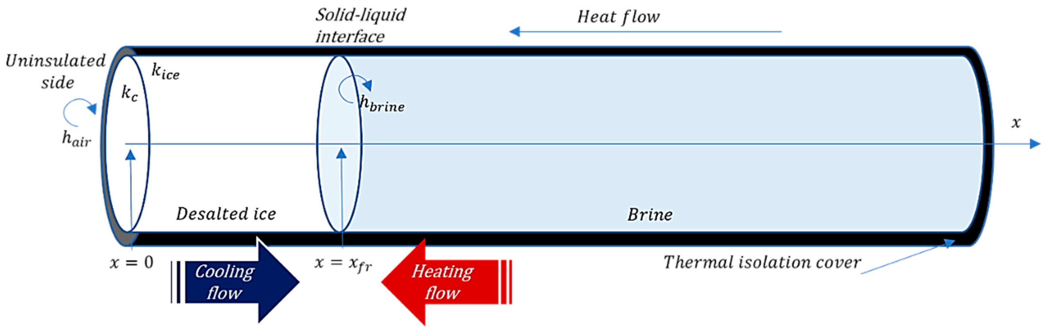
This physical model consists of a horizontal transparent cylinder, thermally insulated, except on one flat side, in order to drive the heat flow in unidimensional x-direction. The non-insulated surface is exposed to the cold air at temperatures ( below the freezing point of the saline solution. Depending on brine and air temperatures, and , respectively, ice formation evolution occurs at the liquid-solid interface. When is below the saline solution freezing point and higher than the temperature of the interface surface of the ice, the heat transfer should occur from brine towards the cold air. The heat transfer is carried out by natural convection between the brine and the ice formed, and the cylinder surface and cold air by conduction through the ice and the thickness of the cylinder material. Figure 1 shows a physical model scheme of the process.
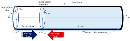
Figure 1.
Scheme of the physical model.
Temperature values and their gradients should be defined in order to:
- Produce ice at the liquid-solid interface, and
- Operate the cooling flow to remove both the latent solidification heat of the water and heat necessary for ice sub-cooling—the correlation between the ice formation kinetics and diffusion time. Ice formation should be performed progressively to allow for the transfer of the ions to the brine.
3. Proposed Model
3.1. Heat Transfer Model Description
3.1.1. Main Equations
Freezing cannot be simulated as a simple general equation of heat conduction, which only governs the solid phase. Therefore, the models are generally formulated for one-dimension thermal conduction for sensible heat transfer.
At , convection heat transfer is performed between the cooling air and the only cylinder surface not insulated, with a cooling rate:
At time t, the freezing interface is located at and Equation (1) is only suitable for . At the convection heat transfer is performed between the brine and the ice surface:
If Equations (1) and (2) are combined, the temperature and global heat flow as a function of and are obtained. The position progression of the ice–brine interface and the heat flow allows for the development of ice production as a function of time at :
where the ratio () is the rate of volume (one-dimensional analysis) of ice formed per unit area on the growing surface (m3/(s m2)), and the expression () is the latent heat fusion per volume (). When the temperature distributions allow the total generated heat flow to be negative, the ice rate increases, and consequently, the value of () is positive.
An adequate analytic solution to these coupled partial differential equations is complicated and may be obtained only for specific cases. Moreover, the particular solution is known for the actual physical conditions on the border. The repartition of temperature modifies the physical and thermal properties of the ice. The homogeneity of the physical properties of the subcooled solid phase (ice) was assumed to simplify the solution (density , heat capacity , conductivity , and thermal diffusivity . Further simplifications were implemented by assuming that the cooling air temperature remains constant. In contrast, the liquid (brine) temperature remained slightly higher than the solidification temperature of the water () and lower than the brine freezing temperature.
The temperature gradients generated, the heat flow rate, acting as thermal resistances in series from the ice, the plate, and the air:
The heat flow rate from the brine is given by Equation (2); it is exclusive of convection heat transfer. Equations (2) and (4) are combined (in Equation (5)) to vanish the heat flow rates:
This manages to relate the ice depth to the freezing time . If the process starts at and continues until the time , the required to increase the of ice generation becomes:
This Equation (6) identifies the time necessary to freeze a brine thickness of x. The ice thickness increase as a function of time implies that the coefficient of dx should be positive.
3.1.2. Complementary Equations
In order to obtain the thermal properties [31], the following equations were used:
It is a function of:
And then, finally:
For both air and brine sides, respectively.
As the saline solution freezing process occurs, the salt, contained homogeneously at the beginning of the process, is displaced towards the non-frozen section; consequently, the brine concentration increases as ice (now free of salt) grows, due to the factors affecting the heat transfer phenomena (described in Equations (7)–(11)), depending on the characteristics of the actual solution.
Sodium chloride (NaCl) was used to estimate the brine behavior because it is the main salt in seawater. Its density, dynamic viscosity, and specific heat agree with the literature values of seawater [32]. The freezing temperature of the brine salt solution was estimated using the equation proposed in [33]:
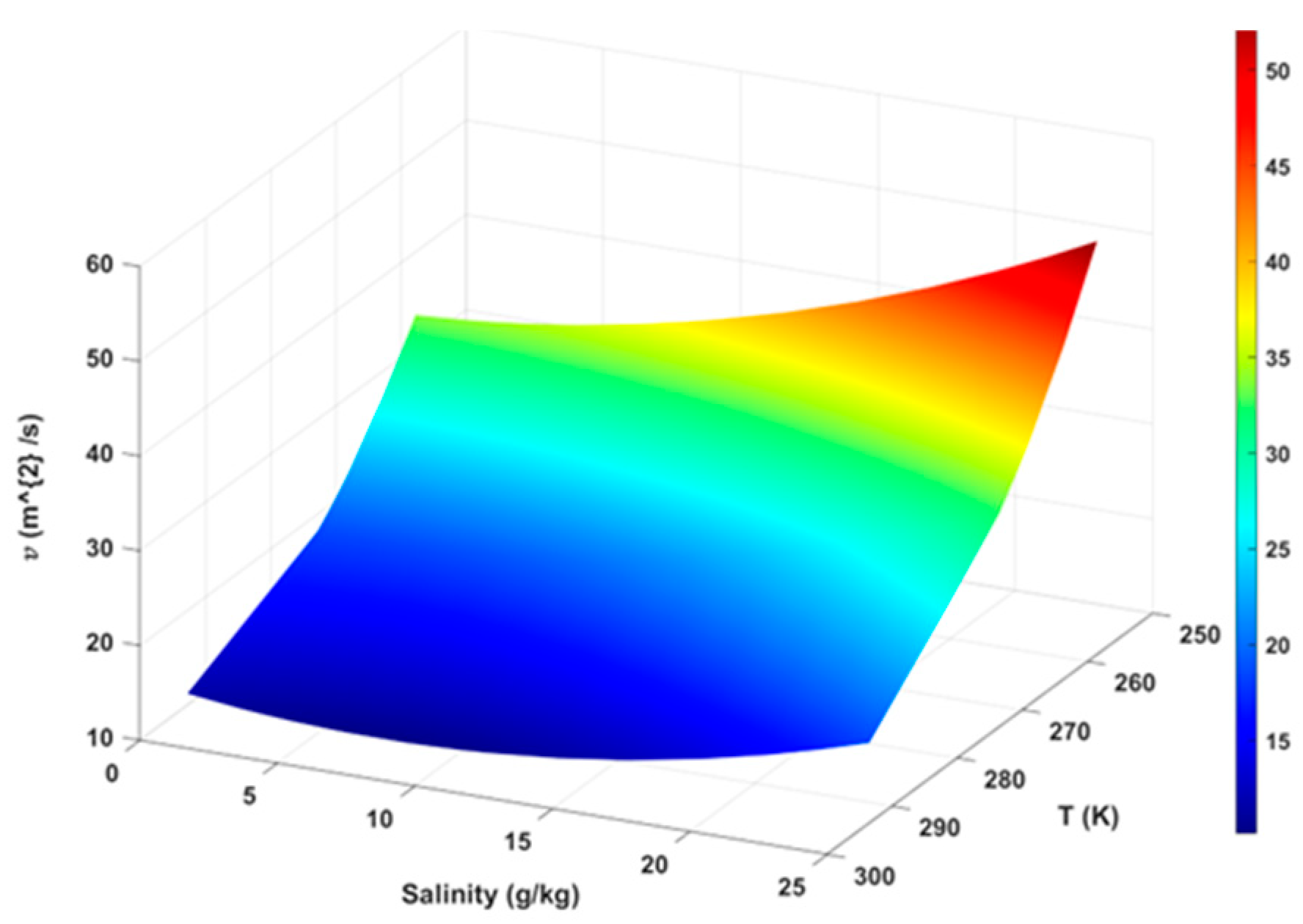
The characteristics of diluted solutions depend mainly on salt concentration. Thus, while salt concentration increases, the freezing point decreases, as can be seen in Figure 2. On the contrary, density, the coefficient of volumetric expansion, kinematic viscosity, thermal conductivity, and osmotic pressure increase with an increase in salinity or temperature [34,35]. Given the lack of information on the properties at seawater below 0 °C, the functions have been collected and extrapolated from sodium chloride-water solutions properties [35,36,37,38], resulting as:
and
for air and brine temperature, respectively.

Figure 2.
Kinematic viscosity*, depending on salinity and temperatures. (See Appendix A).
The equation for the Pr number obtained is μ Cp/k:
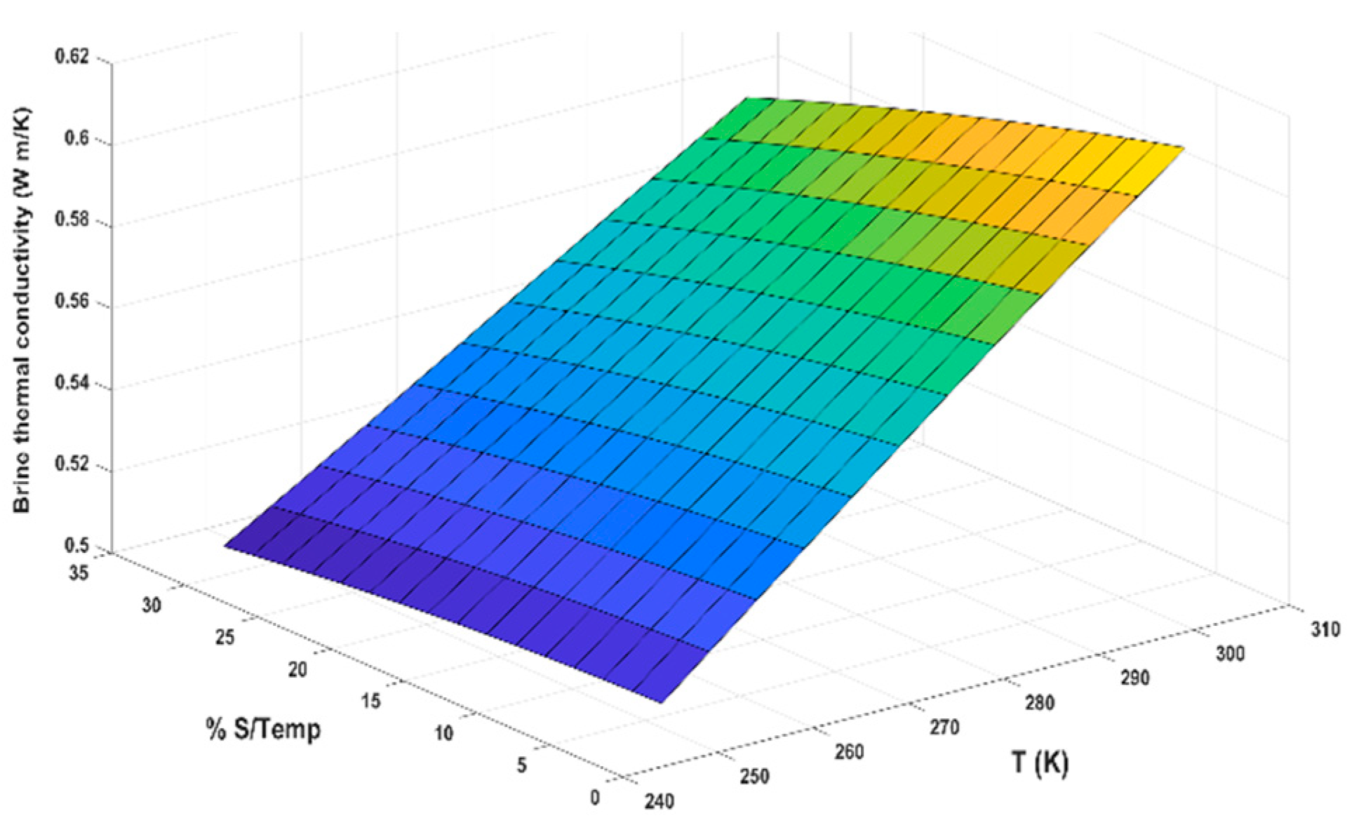
Figure 3 shows the thermal and mass diffusion competition and ion migration at the (at the precise moment of phase change).

Figure 3.
Brine thermal conductivity as a function of salinity and temperature (See Appendix A).
Furthermore, the equations obtained for thermal conductivity is:
The minimum coefficient of multiple correlations for all the equations is R2 = 0.9983.
4. Salt Diffusion Analysis
For salt diffusion during freezing, the model proposed by Allaf is used [39], according to Fick’s law [40]:
The salinity of the solution is ; subsequently, if it is assumed that the water velocity in the brine is global: ≈ 0, and the movement of salt should be uniaxial towards one dimension; Equation (18) becomes:
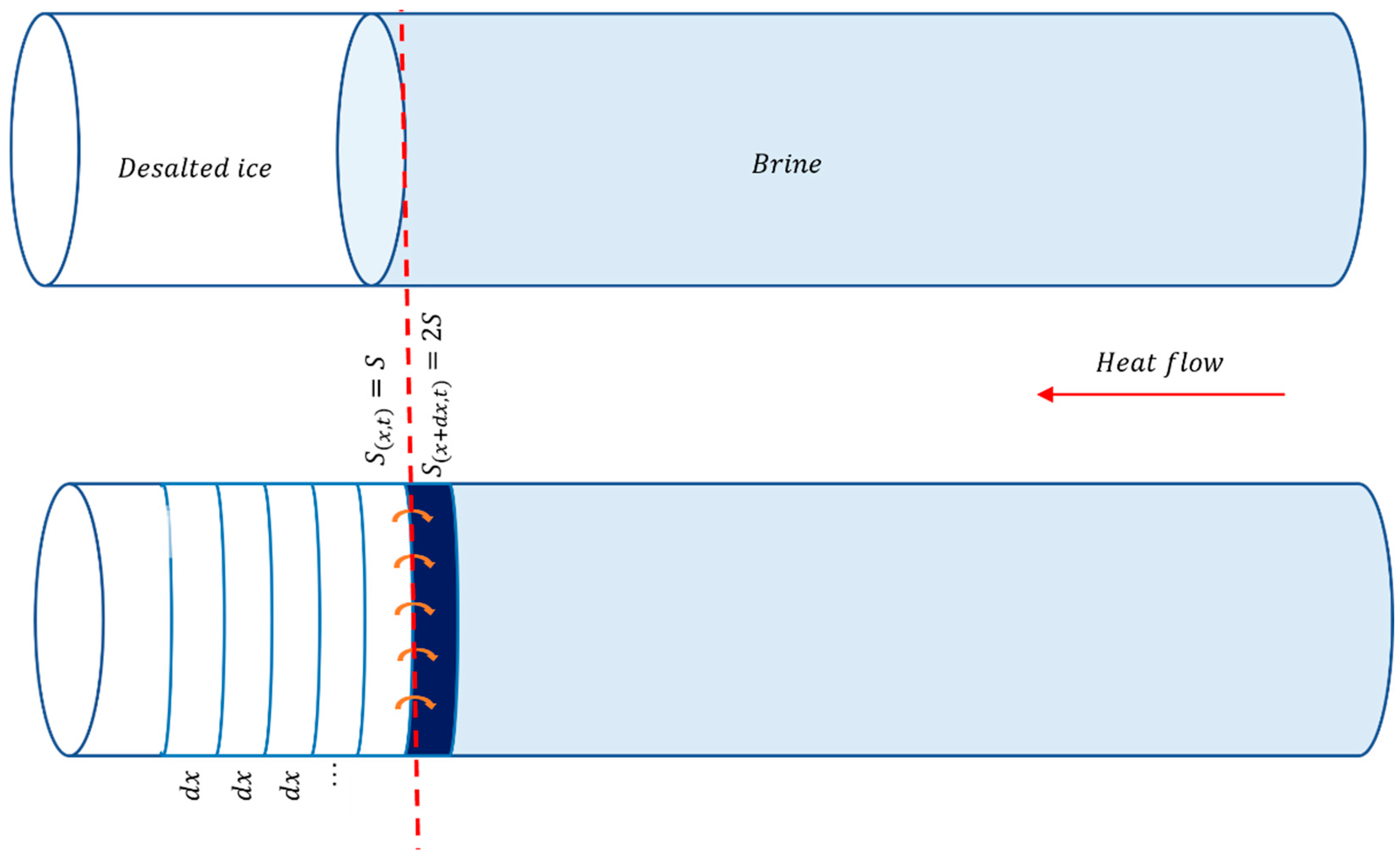
Since the increased ice aims to reach a new equilibrium phase change [41], the solidification process is responsible for the salt’s partial or total expulsion towards the residual, more concentrated brine. The requirement for a complete displacement of salt ions from the dx layer of ice implies that should be twice that of , then:
Therefore, the authors propose:
Then, since the diffusion time is correlated with the dx ice layer, we have:
and:
Thus, the time required for diffusing salt out of the dx layer should be:
Accordingly, the study of mass transfer requires estimating the diffusivity D of salt in the brine. There are several accurate experimental methods for the measurement of D; for example, optical [42], spectroscopic [43], or the Taylor method [44,45]. However, the D value has frequently been estimated due to the expensive instrumentation for each dx, as shown in Figure 4.
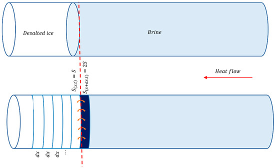
Figure 4.
Thermal vs. mass diffusion competition and ion migration at the interface.
Several literature correlations exist for this purpose [46,47,48,49]. The proposed model uses the Nernst–Haskell equation for electrolyte solutions [49]. The D values found (Table 1) agree with those reported in [18].

Table 1.
Values obtained for the diffusivity of salt in water, temperature, and salinity.
5. Results and Discussions
Conditions for F/M desalination
The F/M process requires at least three essential conditions:
- A positive evolution of growing ice through thickness x:
From Equation (6), since the coefficient should be positive, it is proposed:
Consequently:
Accordingly, Equations (25) and (26) are conditions that strictly depend on air temperature (Tair) and brine temperature (Tb).
- 2.
- Since diffusion time depends on the diffusivity, which is a function of salinity as Equation (23) and Table 1 show, the salinity increases while the value of D decreases.
- 3.
- To get salt-free at a diffusion time lower than freezing time:
Freezing conditions should be carried out to perform ice formation as slowly as possible. This allows the salt ions to “escape” into the brine solution before reaching the solidification of a considered layer (dx).
Salt separation should be considered the most critical condition for appropriate F/M desalination. From the three conditions established, it is possible to regulate the process in terms of the most convenient initial temperatures and salt concentration to allow freezing without salt trapped in frozen water.
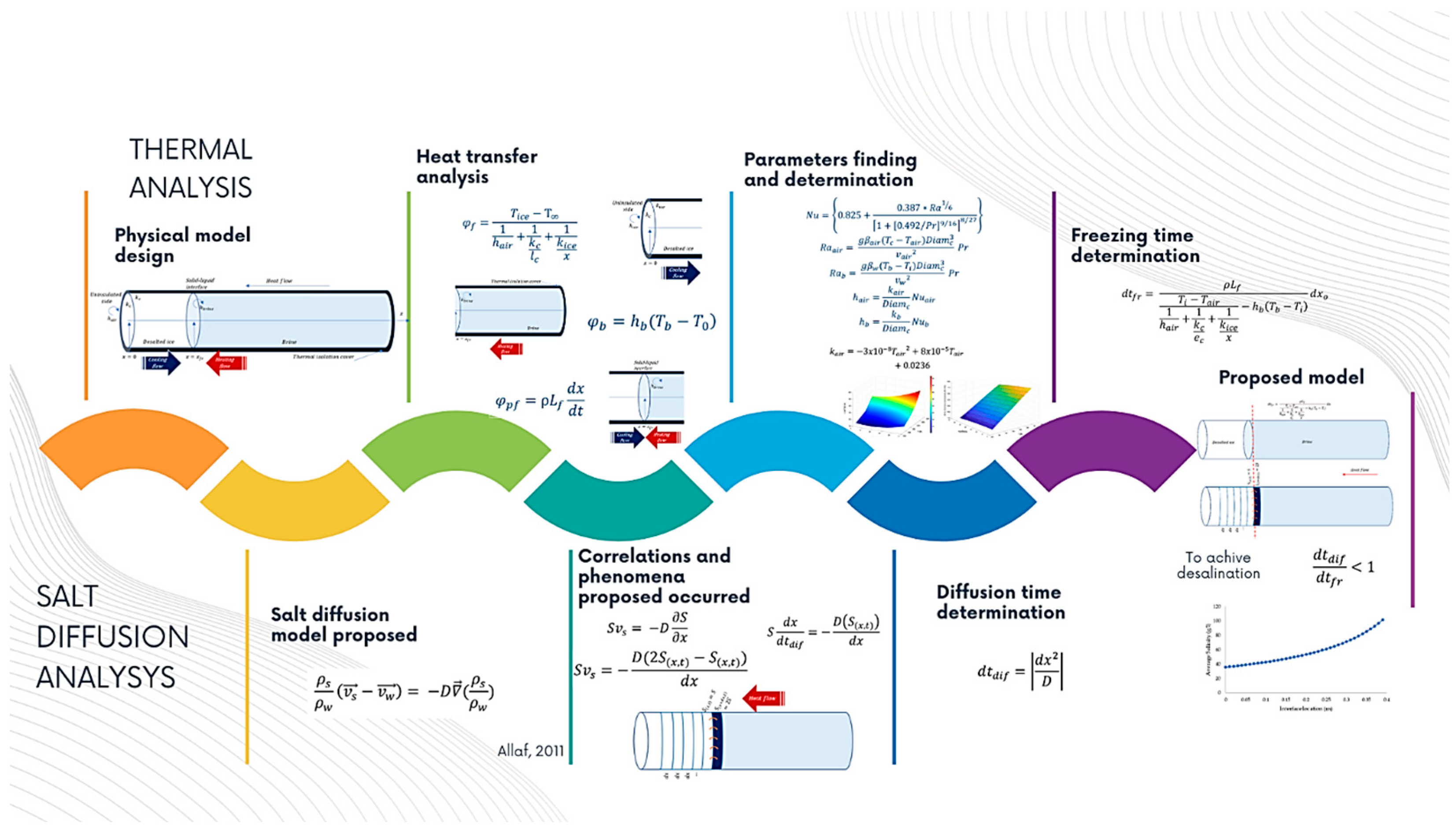
In Figure 5, a schematic flow diagram shows the mass and energy equations for the F/M process; the thermal analysis includes the simultaneous conduction and convection process based on the temperature values of the interface. At the same time, the diffusion process is derived from the salinity values close to the interface zone. Both processes (mass and energy transfer) affect the solidification of the interface, depending on the initial power and salinity.
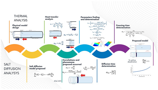
Figure 5.
Schematic flow diagram for the conception of the F/M desalination model.
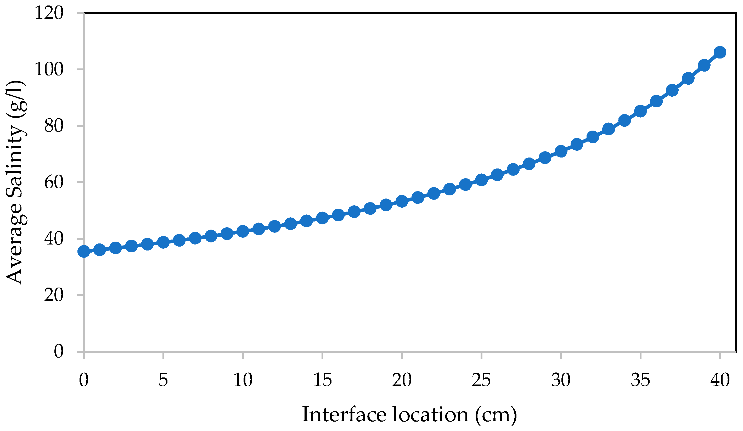
Figure 6 shows the initial salinity condition of 35.5 g/L; as the ice formed increases, the average salinity also increases in the remaining liquid zone. In this case, a 40 cm process for x dimension is presented. At the 5 cm interface location, the salinity does not make a significant mass addition to the liquid section. The NaCl displacement from the initial salinity condition can be observed with a near linear behavior in the first half of the process. A nonlinear effect is shown in the last third of the process, as the solubility diminishes, in agreement with Table 1. The process increases the NaCl salt concentration when the x dimension is finite, and the salt is pushed into the remaining concentrated brine.
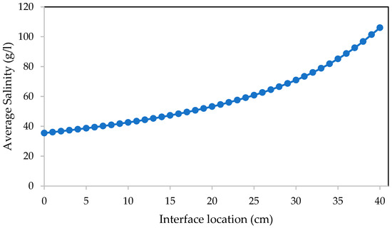
Figure 6.
Brine average salinity, depending on interface location.
In Figure 7, calculated at the initial half x length process, an interface for the initial salinity at 35.5 g/L in the brine (liquid phase) leads to a 112.105 g/L salt concentration in the brine solution. This is the driving force for diffusion from a higher NaCl concentration to the remaining x dimension, which has an average NaCl concentration of 56.0526 g/L.
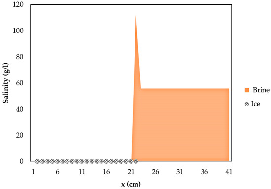
Figure 7.
Salinity profile for 40 cm length process, with an interface at 21 cm.
The model was defined to obtain the conditions required to achieve suitable saline solution desalination. This model is based on comparing both the freezing process and salt diffusion in saline water. It involves the effect of thermal parameters, which generally depend on salt concentration (conductivity, freezing temperature), physical characteristics (density, expansion coefficient, kinematic viscosity, and salt diffusivity), and equipment geometry. The model is simultaneously simple and effective, providing a tool to conduct the F/M desalination process. Important information has been collected to achieve data closer to what is observed during experimentation on a complex problem. For example, the ice growth rate value must be around 3.0 × 10⁻⁷ to achieve ice-salt separation, and the freezing temperature should be below −15 °C to obtain 233 g/L salt concentration in the liquid. This model’s results will help design and build adequate high-performance F/M prototypes and industrial plants.
6. Conclusions
One-dimensional model for the freezing melting process was presented for a freezing water process from NaCl brine solution. The interface moves as slowly as the diffusion salt process allows for the salt-free ice formation, then, the temperature and the new salt concentration have different effects on the interface position. The model equations show a process based on three factors: convection zone, conductivity zone, and mass diffusion.
A slight variation of a one-dimensional thickness (associated with cylinder length) in ice formation results from the convection, conductivity, density, viscosity, and heat for initial temperature and initial salt concentration. A one-dimensional solution assumes the salt gradient is displaced simultaneously with the thermal process; this assumption would be valid for the process in which the container wall is a far distance from the surface once the freezing process has begun, and this is entirely accurate for sea conditions in which the border is far from the surface.
The main discovery of the model is the time required for salt diffusion compared to the time required for phase change in a specific volume of salt water. After a tdif time value, one of them is salt-free, and the mass transfer analysis implies the other volume has a double salt concentration, and then this relatively higher mass potential, according to Fick’s law, pushes the NaCl into the brine, with the initial salt concentration of approximately 8.3 × 10⁻⁶ m2/s for 35.5 g/L.
Author Contributions
B.C.-T.: conceptualization, visualization, methodology, original draft preparation, formal analysis; R.J.R.: conceptualization, visualization, methodology, original draft preparation, formal analysis; K.A.: conceptualization, methodology; I.P.-F.: formal analysis, writing—review, and editing. All authors have read and agreed to the published version of the manuscript.
Funding
This research received no external funding.
Data Availability Statement
Not applicable.
Conflicts of Interest
The authors declare no conflict of interest.
Nomenclature
| a | ice grow rate | m/s |
| x | specific length (x-axis) | m |
| Lf | water heat fusion | J/kg |
| T | temperature | K |
| h | coefficient of heat convection | W/m K |
| heat flux | W/m 2 | |
| k | thermal conductivity | W/m K |
| diffusion velocity | m/s | |
| saltwater diffusivity | m2/s | |
| l | length | m |
| v | kinematic viscosity | m2/s |
| S | salinity | Kg/m3 |
| Pr | Prandtl number | dimensionless |
| Ra | Rayleigh number | dimensionless |
| molecular weight | g/mol | |
| molar volume | m3 mol | |
| t | time | s |
| α | thermal diffusivity | m2/s |
| density | Kg/m3 | |
| coefficient of volumetric expansion | dimensionless | |
| Sub-indices | ||
| i | liquid-solid interface | |
| s | salt | |
| b | brine | |
| fr | freezing | |
| d | diameter | |
| ∞ | infinity | |
| w | water | |
| c | container | |
| air | air | |
| ice | ice | |
Appendix A
Table A1.
Kinematic viscosity ×107 (m2/s) as a function of temperature and salinity.
Table A1.
Kinematic viscosity ×107 (m2/s) as a function of temperature and salinity.
| Temperature (K) | ||||||||||
|---|---|---|---|---|---|---|---|---|---|---|
| Salinity (g/kg) | 293.15 | 273.15 | 272.15 | 271.15 | 270.15 | 269.15 | 268.15 | 263.15 | 258.15 | |
| 0.1 | 11.486 | 18.471 | 19.180 | 19.928 | 20.717 | 21.547 | 22.419 | 27.438 | 33.645 | |
| 2.0 | 10.838 | 18.396 | 19.134 | 19.911 | 20.729 | 21.589 | 22.490 | 27.661 | 34.026 | |
| 2.9 | 10.614 | 18.426 | 19.177 | 19.969 | 20.800 | 21.674 | 22.589 | 27.833 | 34.272 | |
| 4.0 | 10.397 | 18.519 | 19.288 | 20.096 | 20.945 | 21.835 | 22.768 | 28.099 | 34.630 | |
| 5.6 | 10.195 | 18.768 | 19.561 | 20.393 | 21.267 | 22.182 | 23.140 | 28.599 | 35.263 | |
| 6.0 | 10.165 | 18.851 | 19.650 | 20.489 | 21.368 | 22.290 | 23.254 | 28.745 | 35.442 | |
| 8.0 | 10.140 | 19.391 | 20.220 | 21.089 | 22.000 | 22.952 | 23.948 | 29.599 | 36.462 | |
| 8.3 | 10.155 | 19.490 | 20.323 | 21.197 | 22.112 | 23.070 | 24.070 | 29.745 | 36.633 | |
| 10.0 | 10.324 | 20.138 | 20.998 | 21.898 | 22.839 | 23.823 | 24.849 | 30.661 | 37.691 | |
| 11.0 | 10.494 | 20.590 | 21.465 | 22.380 | 23.337 | 24.336 | 25.378 | 31.270 | 38.383 | |
| 13.6 | 11.179 | 22.008 | 22.922 | 23.878 | 24.874 | 25.914 | 26.997 | 33.096 | 40.425 | |
| 16.2 | 12.215 | 23.778 | 24.732 | 25.727 | 26.763 | 27.843 | 28.967 | 35.274 | 42.819 | |
| 18.8 | 13.603 | 25.899 | 26.892 | 27.927 | 29.004 | 30.124 | 31.289 | 37.804 | 45.565 | |
| 21.2 | 15.196 | 28.169 | 29.199 | 30.270 | 31.384 | 32.542 | 33.744 | 40.451 | 48.412 | |
| 23.1 | 16.670 | 30.179 | 31.237 | 32.338 | 33.481 | 34.668 | 35.900 | 42.759 | 50.877 | |
| 24.9 | 18.239 | 32.256 | 33.341 | 34.469 | 35.640 | 36.855 | 38.115 | 45.118 | 53.387 | |
Table A2.
Salted water thermal conductivity (W/m K).
Table A2.
Salted water thermal conductivity (W/m K).
| Temperature (K) | |||||||||||||
|---|---|---|---|---|---|---|---|---|---|---|---|---|---|
| 272.16 | 272.16 | 272.16 | 272.16 | 272.16 | 272.16 | 272.16 | 272.16 | 272.16 | 272.16 | 272.16 | 272.16 | ||
| Salinity (%) | 2 | 0.559 | 0.559 | 0.559 | 0.559 | 0.559 | 0.559 | 0.559 | 0.559 | 0.559 | 0.559 | 0.559 | 0.559 |
| 4 | 0.558 | 0.558 | 0.558 | 0.558 | 0.558 | 0.558 | 0.558 | 0.558 | 0.558 | 0.558 | 0.558 | 0.558 | |
| 6 | 0.557 | 0.557 | 0.557 | 0.557 | 0.557 | 0.557 | 0.557 | 0.557 | 0.557 | 0.557 | 0.557 | 0.557 | |
| 8 | 0.555 | 0.555 | 0.555 | 0.555 | 0.555 | 0.555 | 0.555 | 0.555 | 0.555 | 0.555 | 0.555 | 0.555 | |
| 10 | 0.554 | 0.554 | 0.554 | 0.554 | 0.554 | 0.554 | 0.554 | 0.554 | 0.554 | 0.554 | 0.554 | 0.554 | |
| 12 | 0.553 | 0.553 | 0.553 | 0.553 | 0.553 | 0.553 | 0.553 | 0.553 | 0.553 | 0.553 | 0.553 | 0.553 | |
| 14 | 0.552 | 0.552 | 0.552 | 0.552 | 0.552 | 0.552 | 0.552 | 0.552 | 0.552 | 0.552 | 0.552 | 0.552 | |
| 16 | 0.550 | 0.550 | 0.550 | 0.550 | 0.550 | 0.550 | 0.550 | 0.550 | 0.550 | 0.550 | 0.550 | 0.550 | |
| 18 | 0.549 | 0.549 | 0.549 | 0.549 | 0.549 | 0.549 | 0.549 | 0.549 | 0.549 | 0.549 | 0.549 | 0.549 | |
| 20 | 0.547 | 0.547 | 0.547 | 0.547 | 0.547 | 0.547 | 0.547 | 0.547 | 0.547 | 0.547 | 0.547 | 0.547 | |
| 22 | 0.546 | 0.546 | 0.546 | 0.546 | 0.546 | 0.546 | 0.546 | 0.546 | 0.546 | 0.546 | 0.546 | 0.546 | |
| 24 | 0.544 | 0.544 | 0.544 | 0.544 | 0.544 | 0.544 | 0.544 | 0.544 | 0.544 | 0.544 | 0.544 | 0.544 | |
| 26 | 0.542 | 0.542 | 0.542 | 0.542 | 0.542 | 0.542 | 0.542 | 0.542 | 0.542 | 0.542 | 0.542 | 0.542 | |
| 28 | 0.541 | 0.541 | 0.541 | 0.541 | 0.541 | 0.541 | 0.541 | 0.541 | 0.541 | 0.541 | 0.541 | 0.541 | |
| 30 | 0.539 | 0.539 | 0.539 | 0.539 | 0.539 | 0.539 | 0.539 | 0.539 | 0.539 | 0.539 | 0.539 | 0.539 | |
| 32 | 0.537 | 0.537 | 0.537 | 0.537 | 0.537 | 0.537 | 0.537 | 0.537 | 0.537 | 0.537 | 0.537 | 0.537 | |
References
- Castillo-Téllez, B.; Pilatowsky Figueroa, I.; Castillo Téllez, M.; Marzoug, R.; Allaf, K. Experimental analysis of saline diffusion during saltwater freezing for desalination purposes. Water Environ. J. 2020, 34, 929–936. [Google Scholar] [CrossRef]
- Erlbeck, L.; Rädle, M.; Nessel, R.; Illner, F.; Müller, W.; Rudolph, K.; Kunz, T.; Methner, F.J. Investigation of the depletion of ions through freeze desalination. Desalination 2017, 407, 93–102. [Google Scholar] [CrossRef]
- Liu, Y.; Ming, T.; Wu, Y.; de Richter, R.; Fang, Y.; Zhou, N. Desalination of seawater by spray freezing in a natural draft tower. Desalination 2020, 496, 114700. [Google Scholar] [CrossRef]
- Ghalavand, Y.; Hatamipour, M.S.; Rahimi, A. A review on energy consumption of desalination processes. Desalin. Water Treat. 2015, 54, 1526–1541. [Google Scholar] [CrossRef]
- Do Thi, H.T.; Pasztor, T.; Fozer, D.; Manenti, F.; Toth, A.J. Comparison of Desalination Technologies Using Renewable Energy Sources with Life Cycle, PESTLE, and Multi-Criteria Decision Analyses. Water 2021, 13, 3023. [Google Scholar] [CrossRef]
- Guo, P.; Li, T.; Wang, Y.; Li, J. Energy and exergy analysis of a spray-evaporation multi-effect distillation desalination system. Desalination 2021, 500, 114890. [Google Scholar] [CrossRef]
- Jayakody, H.; Al-Dadah, R.; Mahmoud, S. Numerical investigation of indirect freeze desalination using an ice maker machine. Energy Convers. Manag. 2018, 168, 407–420. [Google Scholar] [CrossRef]
- Yang, H.; Fu, M.; Zhan, Z.; Wang, R.; Jiang, Y. Study on combined freezing-based desalination processes with microwave treatment. Desalination 2020, 475, 114201. [Google Scholar] [CrossRef]
- Ong, C.W.; Chen, C.L. Technical and economic evaluation of seawater freezing desalination using liquefied natural gas. Energy 2019, 181, 429–439. [Google Scholar] [CrossRef]
- Kalista, B.; Shin, H.; Cho, J.; Jang, A. Current development and future prospect review of freeze desalination. Desalination 2018, 447, 167–181. [Google Scholar] [CrossRef]
- Najim, A. A review of advances in freeze desalination and future prospects. NPJ Clean Water 2022, 5, 1–15. [Google Scholar] [CrossRef]
- El Kadi, K.; Janajreh, I. Desalination by Freeze Crystallization: An Overview. Int. J. Therm. Environ. Eng. 2017, 15, 103–110. [Google Scholar] [CrossRef]
- Badawy, S.M. Laboratory freezing desalination of seawater. Desalin. Water Treat. 2016, 57, 11040–11047. [Google Scholar] [CrossRef]
- Chen, J.; Wu, J.; Xu, J.; Yuan, Q.; Deng, B.; Chen, C.; Li, Z. Experiments and insights of desalination by a freezing/thawing method at low subcooling. Chinese J. Chem. Eng. 2020, 28, 3011–3017. [Google Scholar] [CrossRef]
- Jayakody, H.; Al-Dadah, R.; Mahmoud, S. Computational fluid dynamics investigation on indirect contact freeze desalination. Desalination 2017, 420, 21–33. [Google Scholar] [CrossRef]
- Junkratuek, A.; Srudhiprom, J.; Srinophakun, T. Computational fluid dynamics of a horizontal hydrocyclone for freezing desalination. Asia-Pac. J. Chem. Eng. 2017, 12, 765–774. [Google Scholar] [CrossRef]
- El Kadi, K.; Adeyemi, I.; Janajreh, I. Application of directional freezing for seawater desalination: Parametric analysis using experimental and computational methods. Desalination 2021, 520, 115339. [Google Scholar] [CrossRef]
- Yuan, H.; Sun, K.; Wang, K.; Zhang, J.; Zhang, Z.; Zhang, L.; Li, S.; Li, Y. Ice crystal growth in the freezing desalination process of binary water-NaCl system. Desalination 2020, 496, 114737. [Google Scholar] [CrossRef]
- Najim, A.; Krishnan, S. A similarity solution for heat transfer analysis during progressive freeze-concentration based desalination. Int. J. Therm. Sci. 2022, 172, 107328. [Google Scholar] [CrossRef]
- Kapembwa, M.; Rodríguez-Pascual, M.; Lewis, A.E. Heat and Mass Transfer Effects on Ice Growth Mechanisms in Pure Water and Aqueous Solutions. Cryst. Growth Des. 2014, 14, 389–395. [Google Scholar] [CrossRef]
- Savović, S.; Caldwell, J. Finite difference solution of one-dimensional Stefan problem with periodic boundary conditions. Int. J. Heat Mass Transf. 2003, 46, 2911–2916. [Google Scholar] [CrossRef]
- Caldera, U.; Breyer, C. Learning Curve for Seawater Reverse Osmosis Desalination Plants: Capital Cost Trend of the Past, Present, and Future. Water Resour. Res. 2017, 53, 10523–10538. [Google Scholar] [CrossRef]
- Al-sahali, M.; Ettouney, H. Developments in thermal desalination processes: Design, energy, and costing aspects. Desalination 2007, 214, 227–240. [Google Scholar] [CrossRef]
- Thu, K.; Yanagi, H.; Saha, B.B.; Ng, K.C. Performance analysis of a low-temperature waste heat-driven adsorption desalination prototype. Int. J. Heat Mass Transf. 2013, 65, 662–669. [Google Scholar] [CrossRef]
- Narayan, G.P.; Sharqawy, M.H.; Lienhard V, J.H.; Zubair, S.M. Thermodynamic analysis of humidification dehumidification desalination cycles. Desalin. Water Treat. 2010, 16, 339–353. [Google Scholar] [CrossRef]
- Abid, H.S.; Johnson, D.J.; Hashaikeh, R.; Hilal, N. A review of efforts to reduce membrane fouling by control of feed spacer characteristics. Desalination 2017, 420, 384–402. [Google Scholar] [CrossRef]
- Goh, L.M.; Thong, Z.; Li, W.P.; Ooi, S.T.; Esa, F.; Ng, K.S.; Dhalla, A.; Gudipati, C. Development and Industrial-Scale Fabrication of Next-Generation Low-Energy Membranes for Desalination. Membranes 2022, 12, 540. [Google Scholar] [CrossRef]
- Gu, B.; Adjiman, C.S.; Xu, X.Y. The effect of feed spacer geometry on membrane performance and concentration polarisation based on 3D CFD simulations. J. Memb. Sci. 2017, 527, 78–91. [Google Scholar] [CrossRef]
- Shenvi, S.S.; Isloor, A.M.; Ismail, F.F. A review on RO membrane technology: Developments and challenges. Desalination 2015, 368, 10–26. [Google Scholar] [CrossRef]
- Perrins, J.C.; Cooper, W.J.; van Leeuwen, J.; Herwig, R.P. Ozonation of seawater from different locations: Formation and decay of total residual oxidant-implications for ballast water treatment. Mar. Pollut. Bull. 2006, 52, 1023–1033. [Google Scholar] [CrossRef]
- Cengell, Y.; Afshin, G. Transferencia de Calor y Masa, 4th ed.; McGraw Hill: New York, NY, USA, 2011; Volume 1, ISBN 9786071505408. [Google Scholar]
- Melinder, A.; Ignatowicz, M. Properties of seawater with ice slurry use in focus. Int. J. Refrig. 2015, 52, 51–58. [Google Scholar] [CrossRef]
- Fofonoff, N.P. Physical properties of seawater: A new salinity scale and equation of state for seawater. J. Geophys. Res. 1985, 90, 3332. [Google Scholar] [CrossRef]
- Nayar, K.G.; Sharqawy, M.H.; Banchik, L.D.; Lienhard, J.H. Thermophysical properties of seawater: A review and new correlations that include pressure dependence. Desalination 2016, 390, 1–24. [Google Scholar] [CrossRef]
- Simion, A.I.; Grigoraş, C.; Roșu, A. Mathematical modelling of density and viscosity of nacl aqueous solutions. J. Agroaliment. Process. Technol. 2015, 21, 41–52. [Google Scholar]
- Dreith, F.; Raj, M.; Manglik, M.S. Principles of Heat Transfer, 7th ed.; Cengagle Learning, Inc.: Boston, MA, USA, 2011; Volume 2, ISBN 9780495667704. [Google Scholar]
- Melinder, Å. Thermophysical Properties of Aqueous Solutions Used as Secondary Working Fluids, Royal Institute of Technology. Ph.D. Dissertation, KTH, Stockholm, Sweden, 2007. [Google Scholar]
- Cengel, Y.A.; Boles, M.E. Termodinamica, 7th ed.; McGraw Hill: New York, NY, USA, 2011; ISBN 978-607-15-0743-3. [Google Scholar]
- Allaf, K.; Bouyahy, S.M.N.; Romdhane, M. Drying diffusing model. In Proceedings of the 6th International CIGR Technical Symposium—Towards a Sustainable Food Chain: Food Process, Bioprocessing and Food Quality Management, Nantes, France, 18–20 April 2011. [Google Scholar]
- Allaf, K. Transfer Phenomena and Industrial Applications, 1st ed.; Faculty of Science, Lebanese University: Hadath, Lebanon, 1982. [Google Scholar]
- Fukui, K.; Maeda, K. Direct numerical simulation of solid-layer crystallization from binary melt. J. Cryst. Growth 2002, 235, 633–639. [Google Scholar] [CrossRef]
- Krahn, W.; Schwelger, G.; Lucas, K. Light scattering measurements of mutual diffusion coefficients in binary liquid mixtures. J. Phys. Chem. 1983, 87, 4515–4519. [Google Scholar] [CrossRef]
- Stejskal, E.O.; Tanner, J.E. Spin diffusion measurements: Spin echoes in the presence of a time-dependant field gradient. J. Chem. Phys. 1965, 42, 288–292. [Google Scholar] [CrossRef]
- Atwood, J.G.; Goldstein, J. Measurements of Diffusion Coefficients in Liquids at Atmospheric and Elevated Pressure by the Chromatographic Broadening Technique. J. Phys. Chem. 1984, 88, 1875–1885. [Google Scholar] [CrossRef]
- Ouano, C. Diffusion in Liquid Systems. I. A Simple and Fast Method of Measuring Diffusion Constants. Ind. Eng. Chem. Fundam. 1972, 11, 268–271. [Google Scholar] [CrossRef]
- Hayduk, W.; Laudie, H. Prediction of diffusion coefficients for nonelectrolytes in dilute aqueous solutions. AIChE J. 1974, 20, 611–615. [Google Scholar] [CrossRef]
- Miyabe, K.; Isogai, R. Estimation of molecular diffusivity in liquid phase systems by the Wilke-Chang equation. J. Chromatogr. A 2011, 1218, 6639–6645. [Google Scholar] [CrossRef] [PubMed]
- Wilke, C.R.; Chang, P. Correlation of diffusion coefficients in dilute solutions. AIChE J. 1955, 1, 264–270. [Google Scholar] [CrossRef]
- Poling, B.E.; Prausnitz, J.M.; O’Connell, J.P. Properties of Gases and Liquids, 5th ed.; McGraw-Hill Education: New York, NY, USA, 2001; ISBN 9780070116825. [Google Scholar]

Publisher’s Note: MDPI stays neutral with regard to jurisdictional claims in published maps and institutional affiliations. |
© 2022 by the authors. Licensee MDPI, Basel, Switzerland. This article is an open access article distributed under the terms and conditions of the Creative Commons Attribution (CC BY) license (https://creativecommons.org/licenses/by/4.0/).