Identification of Block-Structured Covariance Matrix on an Example of Metabolomic Data

Abstract

Modern investigation techniques (e.g., metabolomic, proteomic, lipidomic, genomic, transcriptomic, phenotypic), allow to collect high-dimensional data, where the number of observations is smaller than the number of features. In such cases, for statistical analyzing, standard methods cannot be applied or lead to ill-conditioned estimators of the covariance matrix. To analyze the data, we need an estimator of the covariance matrix with good properties (e.g., positive definiteness), and therefore covariance matrix identification is crucial. The paper presents an approach to determine the block-structured estimator of the covariance matrix based on an example of metabolomic data on the drought resistance of barley. This method can be used in many fields of science, e.g., in agriculture, medicine, food and nutritional sciences, toxicology, functional genomics and nutrigenomics.

1. Introduction

In many experiments using high-throughput omics technologies, the entire spectrum of the observed features (so-called nontargeted analysis), e.g., chemical compounds, is considered. That leads to collection of a huge amount of data, in which, from statistical point of view, there are too many parameters to estimate (e.g., in metabolomics: [1,2,3,4,5,6], in proteomics: [7,8,9]). Moreover, methods of automated co-eluted compounds separation lead to growing distance between number of features and analyzed samples. To be able to carry out a more detailed statistical analysis for such type of data, a new approach should be adapted. Similar problem (in a simplified version) was considered in [10] by selecting an appropriate covariance structure for three subsets of data obtained in a study of metabolomic changes in barley (Hordeum vulgare) leaves under drought stress. The aim of the work is to present how to proceed metabolites, proteins, lipids, gen expression quantitative traits, phenotypic traits on the example of barley data, to achieve an appropriate covariance structure, which leads to the analysis better reflecting the data. The characterization of a covariance structure was investigated with the use of methods based on the Frobenius norm and on the entropy loss function. In [10] to overcome the problem of singularity, we considered three selected nonsingular subsets of the barley data. In this paper, we analyze the whole dataset working on singular matrix. We indicate block-structured estimators and the most suitable block-structured covariance matrix by visualization of the correlation matrix using heatmaps. The specified block-structured covariance matrices are considered e.g., in [11,12,13].

Analyzing the whole dataset, regarding 781 traits and 211 samples, we have to deal with the problem of high-dimensionality of the data, in which the sample size is too small in comparison to number of variables. All measurements are collected in a matrix $\mathbf{X}\sim N_{m,n}(\mathbf{\mu }\otimes {\mathbf{1}}_n^{\top },\Sigma ,{\mathbf{I}}_n)$, where $\mu$ is a mean vector, $\Sigma$ is a covariance matrix, ${\mathbf{1}}_n$ is an n-dimensional vector of ones and ${\mathbf{I}}_n$ is the identity matrix of order n. To obtain the positive definite (p.d.) covariance matrix estimator, first we need to compute the sample covariance matrix $\mathbf{S}$ defined as

$$\begin{array}{c}\hfill \mathbf{S}=\frac{1}{n}\mathbf{X}\left({\mathbf{I}}_n^{}-\frac{1}{n}{\mathbf{J}}_n\right){\mathbf{X}}^{\top }\end{array}$$

(1)

with ${\mathbf{J}}_n$ is an $n\times n$ matrix of ones. For the analyzed dataset, due to high-dimensionality, the matrix $\mathbf{S}$ is singular. Therefore, we cannot use the entropy loss function, as it was in [10] and we use only the Frobenius norm, where a matrix inversion does not occur.

Our aim is to recognize the structure of the covariance matrix, but the values of the elements of $\mathbf{S}$ are unlimited. Thus, we transform $\mathbf{S}=\left(s_{ij}\right),i,j\in \{1,2,\cdots ,m\}$ to a correlation matrix $\mathbf{R}$ using the following formula:

$$\begin{array}{c}\hfill \mathbf{R}={\mathbf{D}}^{-1}\mathbf{S}{\mathbf{D}}^{-1},\mathrm{where}{\mathbf{D}}^{-1}=\mathrm{diag}\left(\frac{1}{\sqrt{s_{11}}},\frac{1}{\sqrt{s_{22}}},\cdots ,\frac{1}{\sqrt{s_{mm}}}\right).\end{array}$$

(2)

All elements of the matrix $\mathbf{R}$ belong to the interval $[-1,1]$ and for the structure identification, we visualize the correlation matrix using a heatmap (Figure 1).

From Figure 1 we cannot recognize any structure, thus further analysis is necessary. To identify the covariance structure, in the first step, we visualize data using the hierarchical clustering method, which is described in the Section 2.1. Based on the hierarchical clustering results we have described the estimation procedure of the covariance matrix in Section 3 using statistical methods from Section 2.2.

2. Materials and Methods

Our motivation came from an investigation of the effects of water shortage on the levels of primary metabolites in 9 varieties of spring barley, measured repeatedly during drought treatment and control. Data were performed as a pilot study for a larger systems biology project [14]. The pilot experiment is described in [15] for two varieties: Maresi and Cam/B1/CI 08887//CI 05761. Barley plants were cultivated under partially controlled greenhouse conditions. The primary metabolites were recognized by gas chromatography coupled with mass spectrometry (GC–MS). In our paper, nine spring barley genotypes were used: the European varieties Georgia, Maresi, Lubuski, Sebastian and Stratus; Morex, bred in the USA; and Cam/B1/CI 08887//CI 05761, Harmal, and Maris Dingo/Deir Alla 106, being lines bred in Syria. Data were obtained at 4 time points in 4 biological replications and 2 technical replications. The total number of samples was 422. According to [10], after averaging the data over technical replications, 211 samples are obtained and after summation over mass-to-charge ratio, 781 traits are considered. After this step, each biological sample is represented by one total ion current (TIC) chromatogram. In order to ensure normality of the data, observations were transformed by logarithm with base 1.2.

To indicate the most suitable block-structured covariance matrix to our whole dataset, we visualize the data by heatmaps using hierarchical clustering methods, which are described below. Furthermore, in order to indicate block-structured estimators we present methods of its determination.

2.1. Hierarchical Clustering

Due to the fact that the order of random variables is not important in hierarchical clustering, we can change the sequence of variables to find groups of similar traits.

Hierarchical cluster analysis uses a measure of dissimilarity for some number of objects being clustered. Initially, each object is in its own cluster and then the most similar clusters (the smallest dissimilarity) are joined iteratively until there is just a single cluster. At each stage, distances between elements are computed using a selected distance function (described in Section 2.1.1) and the distances between clusters are obtained using the chosen linkage criterion (described in Section 2.1.2). The distances are stored in a distance matrix. The procedure of choosing a pair of clusters to merge at each step is based on finding the nearest clusters (the smallest value) from this distance matrix. We applied R package pvclust [16] to analyze the dissimilarities of the data.

2.1.1. Distance Functions

The distance between two observations can be calculated by the following methods:

• Euclidean—$\sqrt{{\displaystyle \sum _{i=1}^m}{({\mathbf{u}}_i-{\mathbf{v}}_i)}^2}$,
• Maximum—$\underset{i}{max}|{\mathbf{u}}_i-{\mathbf{v}}_i|$,
• Manhattan—${\displaystyle \sum _{i=1}^m}|{\mathbf{u}}_i-{\mathbf{v}}_i|$,
• Canberra—${\displaystyle \sum _{i=1}^m}|{\mathbf{u}}_i-{\mathbf{v}}_i|/|{\mathbf{u}}_i+{\mathbf{v}}_i|$,
• Binary—Jaccard index $J(A,B)=\left(\stackrel{=}{A\cap B}\right)/\left(\stackrel{=}{A\cup B}\right)$—ratio of number of common elements in both sets to number of all elements,
• Minkowski—${\left({\displaystyle \sum _{i=1}^m}{|{\mathbf{u}}_i-{\mathbf{v}}_i|}^k\right)}^{\frac{1}{k}},k\ge 1$.

2.1.2. Linkage Criteria

The following criteria of linkage are implemented:

• Ward.D and Ward.D2—procedures applied the variance analysis to compute the cluster distances. The difference of the two Ward linkage algorithms is that the additional Ward’s clustering criterion is not implemented in “Ward.D” (1963), whereas the option “ward.D2” implements that criterion, with the latter, the dissimilarities are squared before cluster updating; cf. [17],
• Single—procedure computing the distance between two clusters as the minimum distance between each observation from one cluster and each observation from the other cluster,
• Complete—procedure computing the distance between two clusters as the maximum distance between each observation from one cluster and each observation from the other cluster,
• Average (UPGMA—Unweighted Pair-Group Method using Arithmetic Averages)—procedure computing the distance between two clusters as the average distance between each observation from one cluster and each observation from the other cluster,
• Mcquitty (WPGMA—Weighted Pair Group Method with Arithmetic Mean)—procedure based on UPGMA using the size of clusters (number of elements) as weights,
• Centroid (UPGMC—Unweighted Pair-Group Method using the Centroid Average)—the distance between two clusters is the distance between the cluster centroids,
• Median (WPGMC—Weighted Pair-Group Method using the Centroid Average)—procedure based on UPGMC using the size of clusters as weights.

Ward’s minimum variance method points at finding compact spherical clusters. The complete linkage method achieves similar clusters. The single linkage method adopts a “friends of friends” clustering strategy. The other methods can be regarded as aiming for clusters with characteristics somewhere between the single and complete link methods. Note, that the methods median and centroid are not leading to a monotone distance measure, cf. [18].

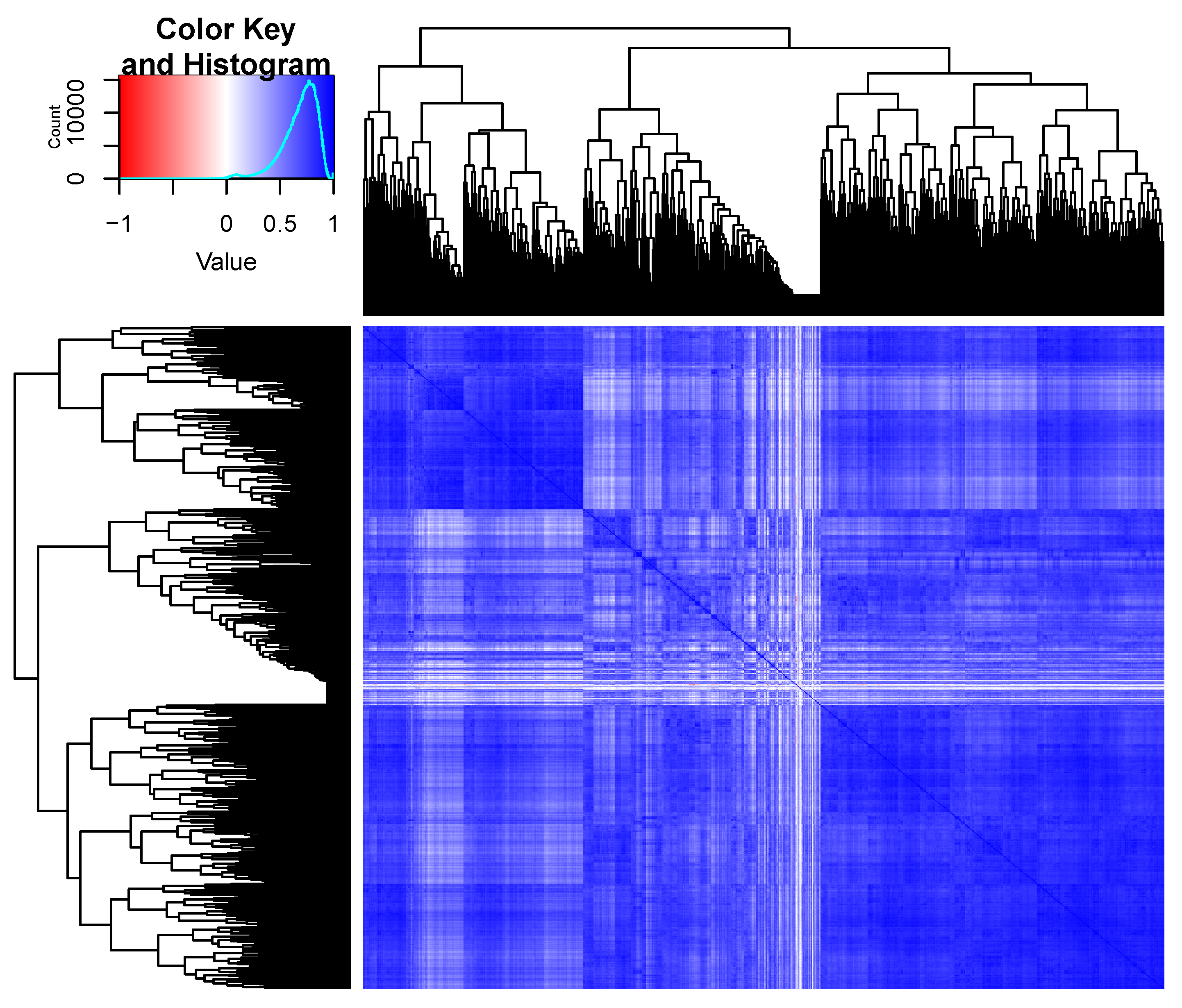
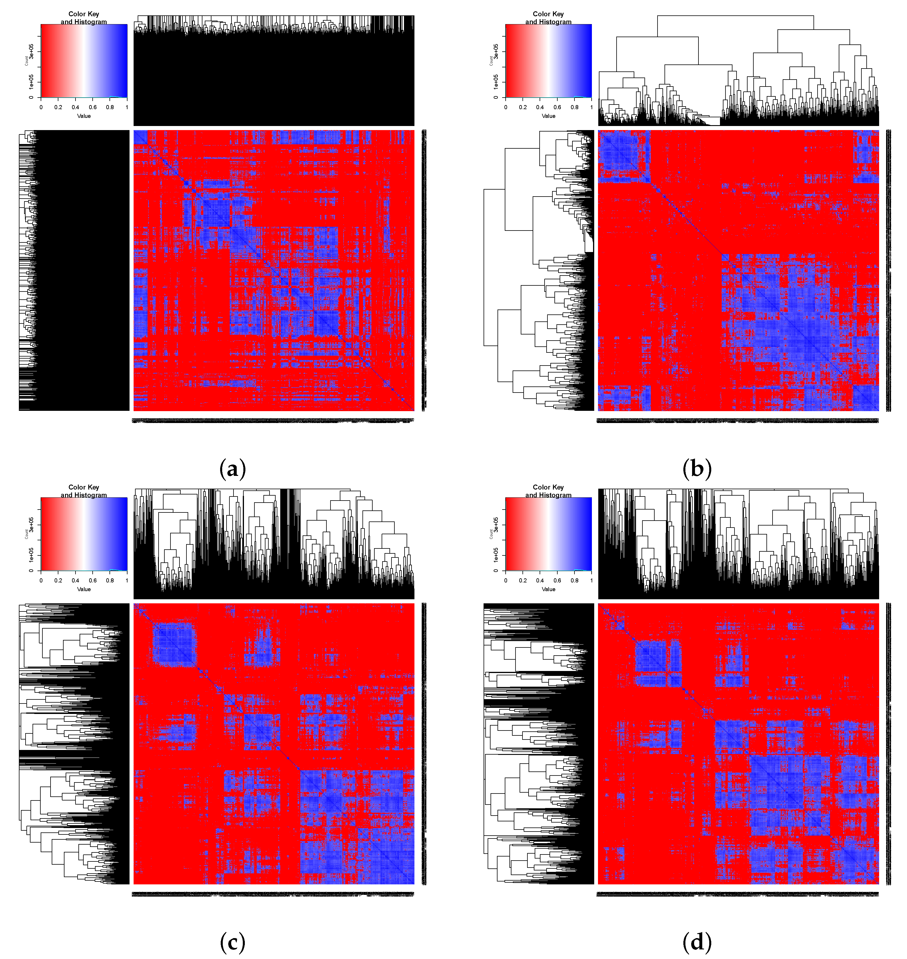
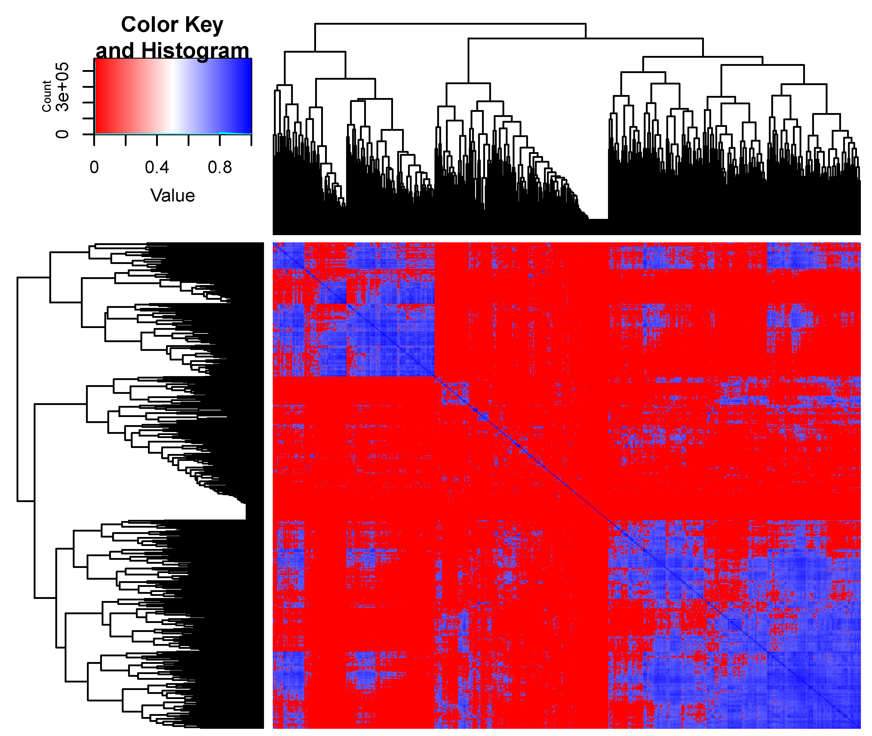
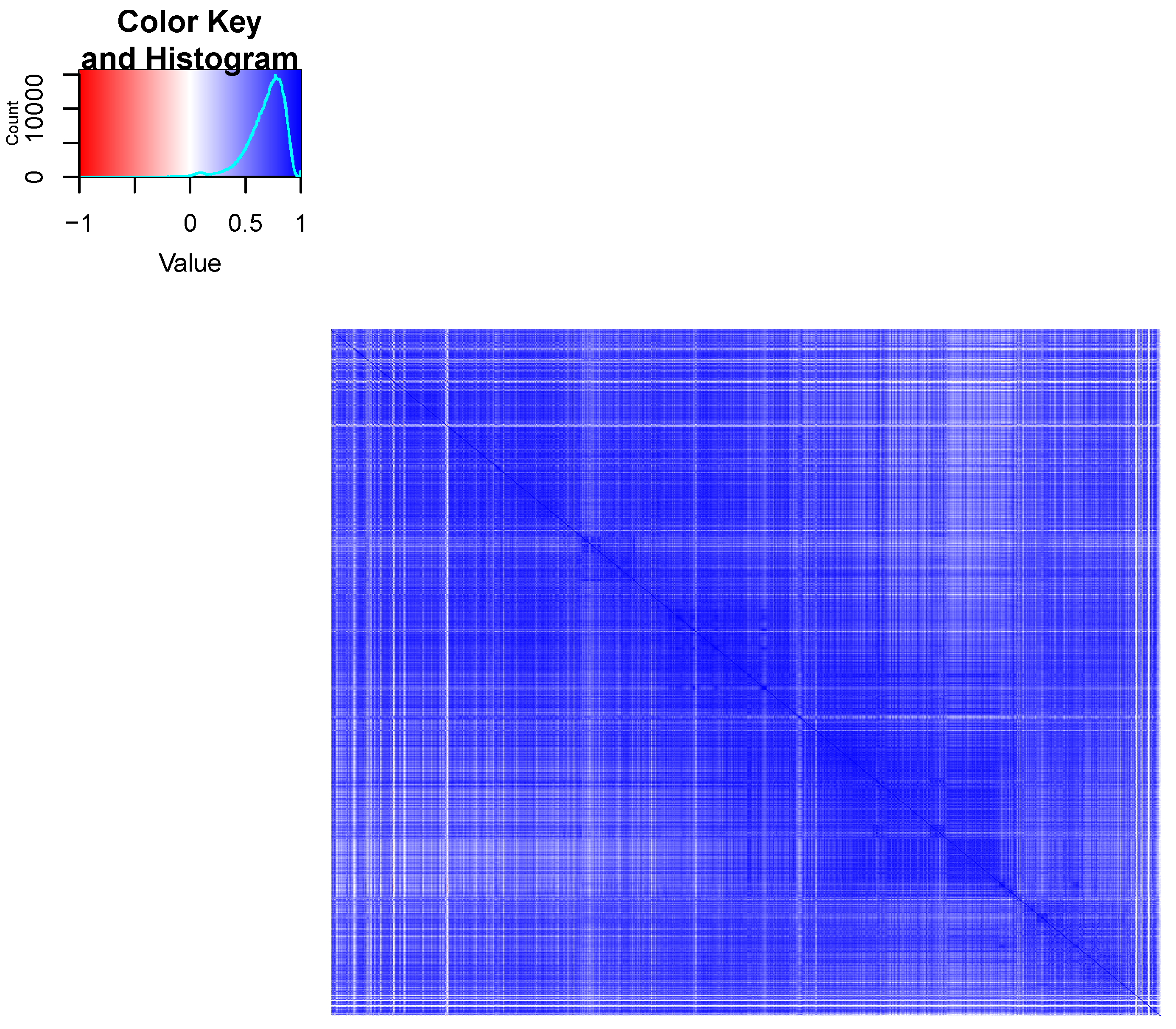
2.1.3. Visualizations

For the matrix $\mathbf{R}$ given in (2) we use hierarchical clustering with the given distance function and linkage criterion to visualize the permuted matrix ${\mathbf{R}}^{*}$, showing in the heatmap presented in Figure 2.

The values of elements of the matrix ${\mathbf{R}}^{*}=\left(r_{i,j}\right),i,j\in \{1,2,\cdots ,m\}$, are very close to each other (see Figure 2). Thus, we applied the thresholding method, where the absolute value of correlations $r_{i,j}$ smaller than $0.8$ are replaced by 0 (only high correlations are interested). Then the features in modified correlation matrix can be grouped in as many ways as the number of combinations of distance functions and the linkage criteria. We cannot indicate which method is the best, since the true covariance matrix is unknown. We visualized the modified correlation matrices using all hierarchical clustering methods for all types of distances. Visualizations help to observe possible block structures. Figure 3 shows four examples.

Obviously, each combination of distance functions and linkage criteria indicates different clusters (Figure 3). In the dendrograms, we can see that for the same linkage criterion, the choice of distance function affects the number of clusters and their abundance. In our opinion, the most suitable structure of the covariance matrix for hierarchical clustering is obtained using complete method with euclidean distance, which is presented in Figure 4. We chose visualization that can be expressed in few simple matrices. Moreover this method and distance are most often used in research.

We can distinguish three diagonal blocks in the covariance matrix structure based on Figure 4. The next section presents the possible covariance structures and methods, which can be used to identify the structure of relevant blocks of the covariance matrix.

2.2. Statistical Background

To deal with the situation, where the number of features m is greater than the number of observations n, we can add a restriction on the covariance matrix structure. In other words, we assume that the covariance matrix has some structure from the set of most common structures described in the next subsection. Further methods of determination estimators of the covariance matrix for a given structure are presented.

2.2.1. Covariance Structures

Let us assume the variances between characteristics are homogenous and the covariances between elements can be homogenous or heterogenous. In the literature different covariance structures with homogenous or heterogenous elements are considered. We choose the most common structures, for which there are methods for obtaining positive definite estimators in the sense of Frobenius norm. Therefore, we consider the following possible covariance structures:

• compound symmetry (CS)

  $$\begin{array}{c}\hfill \begin{array}{ccccc}{\Psi }_{CS}\hfill & =& {\sigma }^2\left(\begin{array}{ccccc}1& \varrho & \varrho & \dots & \varrho \\ \varrho & 1& \varrho & \dots & \varrho \\ \varrho & \varrho & 1& \dots & \varrho \\ ⋮& ⋮& ⋮& \ddots & ⋮\\ \varrho & \varrho & \varrho & \dots & 1\end{array}\right)\hfill & =& {\sigma }^2\left(\varrho {\mathbf{J}}_m+(1-\varrho ){\mathbf{I}}_m^{}\right).\hfill \end{array}\end{array}$$
  To ensure the positive definiteness of the matrix ${\Psi }_{CS}$, we assume ${\sigma }^2>0$ and $\varrho \in \left(-\frac{1}{m-1};1\right)$; cf. [19].
• banded symmetric Toeplitz structure (${\mathbf{T}}_p,p<m$)

  $$\begin{array}{c}\hfill {\Psi }_{T_p}={\sigma }^2\left(\begin{array}{ccccccc}1& {\varrho }_1& \cdots & {\varrho }_p& 0& \cdots & 0\\ {\varrho }_1& 1& {\varrho }_1& \cdots & {\varrho }_p& \ddots & ⋮\\ ⋮& {\varrho }_1& 1& {\varrho }_1& & \ddots & 0\\ {\varrho }_p& & \ddots & \ddots & \ddots & & {\varrho }_p\\ 0& \ddots & & \ddots & \ddots & \ddots & ⋮\\ ⋮& \ddots & \ddots & & \ddots & \ddots & {\varrho }_1\\ 0& \cdots & 0& {\varrho }_p& \cdots & {\varrho }_1& 1\end{array}\right)={\sigma }^2({\mathbf{I}}_m+\sum _{i=1}^p{\varrho }_i{\mathbf{H}}_i),\end{array}$$

  where ${\mathbf{H}}_i$ is an $m\times m$ symmetric matrix with i-th superdiagonal and subdiagonal elements equal to 1 and all other elements equal to 0. In this paper, we consider the Toeplitz covariance matrix with $p=1$ and $p=2$. The matrix ${\Psi }_{T_1}$ is p.d. when

  $$\begin{array}{c}\hfill {\sigma }^2>0\mathrm{and}{\varrho }_1\in \left(-\frac{1}{2cos\frac{\pi }{m+1}};\frac{1}{2cos\frac{\pi }{m+1}}\right).\end{array}$$
  The conditions for positive definiteness of the estimator of the matrix ${\Psi }_{T_p}$ ($p>1$) is not expressed in the explicit form, cf. [20].
• autoregression of order one (AR(1))

  $$\begin{array}{c}\hfill \begin{array}{c}{\Psi }_{AR}={\sigma }^2\left(\begin{array}{ccccc}1& \varrho & {\varrho }^2& \dots & {\varrho }^{m-1}\\ \varrho & 1& \varrho & \dots & {\varrho }^{m-2}\\ {\varrho }^2& \varrho & 1& \dots & {\varrho }^{m-3}\\ ⋮& ⋮& ⋮& \ddots & ⋮\\ {\varrho }^{m-1}& {\varrho }^{m-2}& {\varrho }^{m-3}& \dots & 1\end{array}\right)={\sigma }^2{\displaystyle \sum _{i=0}^{m-1}}{\varrho }^i{\mathbf{H}}_i\hfill \end{array}\end{array}$$

  with ${\mathbf{H}}_0={\mathbf{I}}_m$. The matrix ${\Psi }_{AR}$ is p.d. when we assume ${\sigma }^2>0$ and $\varrho \in \left(-1;1\right)$; cf. [19]. The AR(1) structure is a special case of Toeplitz matrices with $p=m-1$.

2.2.2. Identification Methods

In the paper [10], where the nonsingular matrices were considered, besides the Frobenius norm, the entropy loss function was used as an identification method. This discrepancy function was considered also in [19] for standard multivariate model, and in [21,22] or [23] for doubly multivariate model. However, the entropy loss function requires nonsingularity of the observation matrix and it cannot be applied for considered dataset.

To find the most suitable covariance structure, we use the Frobenius norm

$$\begin{array}{c}\hfill f_F(\mathbf{S},\Psi )=\left|\right|\mathbf{S}-{\Psi \left|\right|}_F=\sqrt{tr\left[\left(\mathbf{S}-\Psi \right){\left(\mathbf{S}-\Psi \right)}^{\top }\right]}.\end{array}$$

The formulae for the p.d. estimator of a structured covariance matrix using the Frobenius norm are described by [24] for CS, ${\mathrm{T}}_1$ and AR(1) and by [20] for ${\mathrm{T}}_p$. These formulae are as follows:

• CS structure

  $$\begin{array}{c}\hfill \left\{\begin{array}{ccc}{\displaystyle \varrho }\hfill & =& {\displaystyle \frac{\delta }{(m-1)tr\left(\mathbf{S}\right)}}\hfill \\ {\displaystyle {\sigma }^2}\hfill & =& {\displaystyle \frac{tr\left(\mathbf{S}\right)+\varrho \delta }{m+m(m-1){\varrho }^2}}\hfill \end{array}\right.\end{array}$$

  with $\delta =tr\left[\mathbf{S}\left({\mathbf{J}}_m-{\mathbf{I}}_m\right)\right]$,
• Toeplitz structure

  ○

  ${\mathrm{T}}_p$ for $p=1$

  $$\begin{array}{c}\hfill \left\{\begin{array}{ccc}{\displaystyle {\sigma }^2}\hfill & =& {\displaystyle \frac{tr\left(\mathbf{S}\right)}{m}}\hfill \\ {\displaystyle {\varrho }_1}\hfill & =& {\displaystyle \frac{mtr\left(\mathbf{S}{\mathbf{H}}_1\right)}{2(m-1)tr\left(\mathbf{S}\right)}}\hfill \end{array}\right.\end{array}$$

  (3)

  Ref. [20] observed that the matrix obtained from (3) given by [24] may be indefinite. Thus, they proposed an algorithm for determination of the minimum of the Frobenius norm; cf. Filipiak et al. (2018d), p. 77. It can be shown that for the ${\sigma }^2$ and ${\varrho }_1$ given in (3), the estimator of ${\mathrm{T}}_1$ can be given as

  $$\begin{array}{c}\hfill t{\sigma }^2\left({\mathbf{I}}_m+\frac{1}{2cos\frac{\pi }{m+1}}{\mathbf{H}}_1\right)\mathrm{if}{\varrho }_1>0\end{array}$$

  and

  $$\begin{array}{c}\hfill t{\sigma }^2\left({\mathbf{I}}_m-\frac{1}{2cos\frac{\pi }{m+1}}{\mathbf{H}}_1\right)\mathrm{if}{\varrho }_1<0\end{array}$$

  with

  $$\begin{array}{c}\hfill t=\left(m+\frac{{\varrho }_1(m-1)}{cos\frac{\pi }{m+1}}\right)/\left(m+\frac{m-1}{2{(cos\frac{\pi }{m+1})}^2}\right).\end{array}$$

  ○

  ${\mathrm{T}}_p$ for $p>1$

  In this case, the formulae for the estimator of the ${\mathrm{T}}_p$ structure cannot be given in explicit form. To determine the estimator, the algorithm proposed by [20], p. 78, can be used.

• AR(1) structure
  To determine the estimator of the AR(1) structure, the following system of equations should be solved:

  $$\begin{array}{c}\hfill \left\{\begin{array}{c}{\displaystyle -\sum _{i=1}^{m-1}i{\varrho }^{i-1}tr\left({\mathbf{SH}}_i\right)+\frac{2{\displaystyle \sum _{i=0}^{m-1}}{\varrho }^{i}tr\left({\mathbf{SH}}_i\right){\displaystyle \sum _{i=1}^{m-1}}(m-i)i{\varrho }^{2i-1}}{m+2{\displaystyle \sum _{i=1}^{m-1}}(m-i){\varrho }^{2i}}=0}\hfill \\ {\displaystyle {\sigma }^2=\frac{{\displaystyle \sum _{i=0}^{m-1}}{\varrho }^{i}tr\left({\mathbf{SH}}_i\right)}{m+2{\displaystyle \sum _{i=1}^{m-1}}(m-i){\varrho }^{2i}}}\hfill \end{array}\right.\end{array}$$

  with ${\mathbf{H}}_0={\mathbf{I}}_m$. The above system of equations provides the local minimum of the discrepancy function; cf. [24].

For CS and AR(1), the formulae described by [25] relating to the separable structure $\Psi \otimes \Sigma$ ($\Psi :p\times p$ and $\Sigma :q\times q$) with $q=1$ can also be used.

3. Results

The first step of the structure identification is choosing the number of diagonal blocks b, based on the heatmaps (for example, three or four). Depending on the number of considered structures a, the number of possible combinations on diagonal is $a^b$. We consider four structures and additionally we have the scaled identity matrix, therefore $5^b$ combinations of diagonal block structures are possible. Off-diagonal blocks are rectangular matrices consisting of zeros or nonzero values. Because the covariance matrix and its estimator are symmetric, thus we have $5^b\times 2^{b(b-1)/2}$ possible combinations to consider.

In the next part of this section, we show the feasible way to obtain the closest estimator in the sense of Frobenius norm. Surely, if we have a few estimators with nearby distances of Frobenius norm, we should select the structure, which explains in the best way the nature of the phenomenon under investigation.

For the considered data, we chose three diagonal blocks (1000 possible structures to consider) based on the Figure 4. This visualization is determined by one particular permutation of $\mathbf{R}$. Therefore we have to use the same permutation for $\mathbf{S}$ and we denote it as ${\mathbf{S}}^{*}$.

Firstly, we assume the following structure of ${\mathbf{S}}^{*}$:

$${\Sigma }_1=\left(\begin{array}{ccc}{\Sigma }_{11}& \mathbf{0}& \mathbf{0}\\ \mathbf{0}& {\Sigma }_{22}& \mathbf{0}\\ \mathbf{0}& \mathbf{0}& {\Sigma }_{33}\end{array}\right)$$

with

$$\begin{array}{ccc}{\Sigma }_{11}& =& {\Psi }_1:215\times 215,\hfill \\ {\Sigma }_{22}& =& {\sigma }_2^2{\mathbf{I}}_{231},\hfill \\ {\Sigma }_{33}& =& {\Psi }_3:335\times 335.\hfill \end{array}$$

For different structures for diagonal blocks ${\Psi }_1$ and ${\Psi }_3$ we compute the Frobenius norm distances between ${\mathbf{S}}^{*}$ and ${\Sigma }_1$. However, the Frobenius norm is not an upper bounded distance and we cannot conclude that we are close or far from the true structure. Thus, we use the adjusted Frobenius norm of the form

$$f_F({\mathbf{S}}^{*},\Psi )/\left|\right|{\mathbf{S}}^{*}{\left|\right|}_F,$$

which has values from the interval [0,1]; cf. [21,25]. We can interpret a small value (near 0) of the adjusted distance as the considered structure is close to the true structure and a value close to 1, that the considered structure is far from the true structure. It is worth noting that, $\left|\right|{\mathbf{S}}^{*}{\left|\right|}_F={\left|\right|\mathbf{S}\left|\right|}_F$ in our case.

The adjusted Frobenius norm distances between ${\mathbf{S}}^{*}$ and ${\Sigma }_1$ with different (optimal) diagonal blocks are presented in

Table 1. Adjusted Frobenius norm distances between ${\mathbf{S}}^{*}$ and ${\Sigma }_1$.

	${\mathbf{\Psi }}_3$	$\mathit{CS}$	$\mathit{AR}\left(1\right)$	${\mathit{T}}_1$	${\mathit{T}}_2$
${\mathbf{\Psi }}_1$
$CS$		0.81877	0.81892	0.93560	0.93492
$AR\left(1\right)$		0.81882	0.81898	0.93565	0.93497
$T_1$		0.88871	0.88885	0.99738	0.99674
$T_2$		0.88805	0.88820	0.99680	0.99616

.

The smallest distance between ${\mathbf{S}}^{*}$ and ${\Sigma }_1$ is observed for ${\Sigma }_{11}$ and ${\Sigma }_{33}$ having CS structures with parameters given in

Table 2. Parameter values of ${\tilde{\Sigma }}_1$.

	${\tilde{\mathbf{\Sigma }}}_{11}$	${\tilde{\mathbf{\Sigma }}}_{22}$	${\tilde{\mathbf{\Sigma }}}_{33}$
${\tilde{\sigma }}_i^2$	31.4724	29.14777	26.4708
${\tilde{\varrho }}_i$	0.7920	–	0.7897

.

It is worth noting that the ${\Sigma }_1$ is a positive definite matrix, because all diagonal blocks are p.d.

In ${\Sigma }_1$ we assume, that ${\Sigma }_{22}$ is scaled identity matrix. However, we should examine other structures. Thus, we assume the following block structure:

$${\Sigma }_2=\left(\begin{array}{ccc}{\Sigma }_{11}& \mathbf{0}& \mathbf{0}\\ \mathbf{0}& {\Sigma }_{22}& \mathbf{0}\\ \mathbf{0}& \mathbf{0}& {\Sigma }_{33}\end{array}\right)$$

with

$$\begin{array}{ccc}{\Sigma }_{11}& =& {\sigma }_1^2({\rho }_1{\mathbf{J}}_{215}+(1-{\rho }_1){\mathbf{I}}_{215}),\hfill \\ {\Sigma }_{22}& =& {\Psi }_2:231\times 231,\hfill \\ {\Sigma }_{33}& =& {\sigma }_3^2({\rho }_3{\mathbf{J}}_{335}+(1-{\rho }_3){\mathbf{I}}_{335}).\hfill \end{array}$$

The adjusted Frobenius norm distances between ${\mathbf{S}}^{*}$ and ${\Sigma }_2$ with different ${\Sigma }_{22}$ structures are presented in

Table 3. Adjusted Frobenius norm distances between ${\mathbf{S}}^{*}$ and ${\Sigma }_2$.

${\mathbf{\Psi }}_2$	$\mathit{CS}$	$\mathit{AR}\left(1\right)$	${\mathit{T}}_1$	${\mathit{T}}_2$
$f_F({\mathbf{S}}^{*},{\Sigma }_2)/\left|\right|{\mathbf{S}}^{*}{\left|\right|}_F$	0.79225	0.79249	0.81832	0.81794

.

The smallest distance is for ${\Sigma }_{22}$ being the CS structure with ${\tilde{\sigma }}_2^2=29.1478$ and ${\tilde{\varrho }}_2=0.4736$. Clearly, the ${\Sigma }_2$ is also p.d., since ${\Sigma }_{22}$ is p.d.

So far, we considered the off-diagonal blocks being zero matrices. Currently, we assume that these blocks are rectangular matrices with all elements equal ${\delta }_i,i=1,2,3$. Thus, we assume the following block structure:

$${\Sigma }_3=\left(\begin{array}{ccc}{\Sigma }_{11}& {\Sigma }_{12}& {\Sigma }_{13}\\ {\Sigma }_{12}^{\top }& {\Sigma }_{22}& {\Sigma }_{23}\\ {\Sigma }_{13}^{\top }& {\Sigma }_{23}^{\top }& {\Sigma }_{33}\end{array}\right)$$

with

$$\begin{array}{ccc}{\Sigma }_{11}& =& {\sigma }_1^2({\rho }_1{\mathbf{J}}_{215}+(1-{\rho }_1){\mathbf{I}}_{215}),\hfill \\ {\Sigma }_{22}& =& {\sigma }_2^2({\rho }_2{\mathbf{J}}_{231}+(1-{\rho }_2){\mathbf{I}}_{231}),\hfill \\ {\Sigma }_{33}& =& {\sigma }_3^2({\rho }_3{\mathbf{J}}_{335}+(1-{\rho }_3){\mathbf{I}}_{335}),\hfill \\ {\Sigma }_{12}& =& {\delta }_1{\mathbf{1}}_{215}^{}{\mathbf{1}}_{231}^{\top },\hfill \\ {\Sigma }_{13}& =& {\delta }_2{\mathbf{1}}_{215}^{}{\mathbf{1}}_{335}^{\top },\hfill \\ {\Sigma }_{23}& =& {\delta }_3{\mathbf{1}}_{231}^{}{\mathbf{1}}_{335}^{\top }.\hfill \end{array}$$

The smallest distance between ${\mathbf{S}}^{*}$ and ${\Sigma }_3$ is equal $0.37952$ for ${\delta }_i$ presented in the

Table 4. Parameter values for ${\tilde{\delta }}_i,i=1,2,3$.

	${\tilde{\mathbf{\Sigma }}}_{12}$	${\tilde{\mathbf{\Sigma }}}_{13}$	${\tilde{\mathbf{\Sigma }}}_{23}$
${\tilde{\delta }}_i$	14.7186	18.5793	16.7440

.

The distance between ${\mathbf{S}}^{*}$ and ${\Sigma }_3$ is much smaller than between ${\mathbf{S}}^{*}$ and previously considered structures ${\Sigma }_1$ and ${\Sigma }_2$.

It should be emphasized that the matrix ${\Sigma }_3$ can be indefinite. Thus we should check the positive definiteness of the obtained estimator. In considered case ${\Sigma }_3$ is p.d. If ${\Sigma }_3$ is not positive definite, then we will modify the off-diagonal blocks, to get p.d. estimator. We propose to multiply off-diagonal blocks by a number from the interval $(0,1)$, such that the estimator is p.d. and the Frobenius norm is as small as possible.

Let us recall that we were looking for the estimator of ${\mathbf{S}}^{*}$, which is permuted $\mathbf{S}$. To get the estimator of the matrix $\mathbf{S}$ we should inverse the permutation, which means in this case using the same permutation again: $\mathbf{S}={\left({\mathbf{S}}^{*}\right)}^{*}$. The estimator of $\mathbf{S}$ has the same eigenvalues as the estimator of ${\mathbf{S}}^{*}$, since the applied permutation is even. Therefore the estimator of $\mathbf{S}$ is also p.d.

4. Discussion

The problem was considered in [10] for three selected nonsingular subsets of the barley data. However, more interested is whole dataset, which is usually singular in high-dimensional case. The results of selected subsets are uncomparable with the results of all dataset. For the first considered diagonal structure ${\Sigma }_1$ we obtained the smallest adjusted Frobenius norm equals $0.81877$. Adding one more diagonal structure the distance is $0.79225$. Taking into account non-zeros off-diagonal blocks the best result is $0.37952$, which gives significant improvement.

The structure analysis of the estimator ${\Sigma }_3$ show that some metabolomic groups are identically correlated and the number of parameters was reduced from $781\times (781+1)/2$ to 9. Obviously, using more diagonal blocks, we will estimate more parameters of the covariance matrix and we should obtain a closest estimator in the sense of the Frobenius norm.

5. Conclusions

By analyzing experiments where many characteristics are measured, the existing dependencies between the variables should be taken into account. The covariance matrix identification allows us to expand knowledge about feature dependencies and enables data analyzing using a more precise statistical model with a smaller number of covariance parameters. It is particularly important in high-dimensional problems where standard methods are not always available, since the matrix $\mathbf{S}$ is, in almost all cases, singular. The knowledge of the estimator of the covariance matrix with good properties is crucial in many statistical analysis methods, e.g., principal component analysis (PCA), linear or quadratic discriminant analysis (LDA or QDA), regression analysis, analysis of independence and conditional independence relationships between components.

Visualisation of correlation matrices using heatmaps is useful in finding block- structured estimators and facilitates the selection of an appropriate structure to the statistical model. In this paper, metabolomic data obtained by GC-MS technique were used. However, our approach can be applied to any type of high-dimensional data, e.g., obtained by different omics techniques, namely: metabolomics, proteomics, limidomics, genomics and transcyptomics as well as common phenotypic data. Moreover, the obtained covariance matrix estimator can be used in aforementioned methods of statistical analysis.

References

1. Winkelmüller, T.M.; Entila, F.; Anver, S.; Piasecka, A.; Song, B.; Dahms, E.; Sakakibara, H.; Gan, X.; Kułak, K.; Sawikowska, A.; et al. Gene expression evolution in pattern-triggered immunity within Arabidopsis thaliana and across Brassicaceae species. Plant Cell 2021, 33, 1863–1887. [Google Scholar] [CrossRef] [PubMed]
2. Piasecka, A.; Sawikowska, A.; Kuczyńska, A.; Ogrodowicz, P.; Mikołajczak, K.; Krajewski, P.; Kachlicki, P. Phenolic metabolites from barley in contribution to phenome in soil moisture deficit. Int. J. Mol. Sci. 2020, 21, 6032. [Google Scholar] [CrossRef]
3. Sawikowska, A.; Piasecka, A.; Kachlicki, P.; Krajewski, P. Separation of chromatographic co-eluted compounds by clustering and by functional data analysis. Metabolites 2021, 11, 214. [Google Scholar] [CrossRef]
4. Kruszka, D.; Sawikowska, A.; Selvakesavan, R.K.; Krajewski, P.; Kachlicki, P.; Franklin, G. Silver nanoparticles affect phenolic and phytoalexin composition of Arabidopsis thaliana. Sci. Total Environ. 2020, 716, 135361. [Google Scholar] [CrossRef]
5. Piasecka, A.; Sawikowska, A.; Kuczyńska, A.; Ogrodowicz, P.; Mikołajczak, K.; Krystowiak, K.; Gudyś, K.; Guzy-Wróbelska, J.; Krajewski, P.; Kachlicki, P. Drought related secondary metabolites of barley (Hordeum vulgare L.) leaves and their association with mQTLs. Plant J. 2017, 89, 898–913. [Google Scholar] [CrossRef] [PubMed] [Green Version]
6. Garibay-Hernández, A.; Kessler, N.; Józefowicz, A.M.; Türksoy, G.M.; Lohwasser, U.; Mock, H.-P. Untargeted metabotyping to study phenylpropanoid diversity in crop plants. Physiol. Plant. 2021, 173, 680–697. [Google Scholar] [CrossRef]
7. Tracz, J.; Handschuh, L.; Lalowski, M.; Marczak, Ł.; Kostka-Jeziorny, K.; Perek, B.; Wanic-Kossowska, M.; Podkowińska, A.; Tykarski, A.; Formanowicz, D.; et al. Proteomic Profiling of Leukocytes Reveals Dysregulation of Adhesion and Integrin Proteins in Chronic Kidney Disease-Related Atherosclerosis. J. Proteome Res. 2021, 20, 3053–3067. [Google Scholar] [CrossRef]
8. Thompson, R.M.; Dytfeld, D.; Reyes, L.; Robinson, R.M.; Smith, B.; Manevich, Y.; Jakubowiak, A.; Komarnicki, M.; Przybylowicz-Chalecka, A.; Szczepaniak, T.; et al. Glutaminase inhibitor CB-839 synergizes with carfilzomib in resistant multiple myeloma cells. Oncotarget 2017, 8, 35863–35876. [Google Scholar] [CrossRef] [Green Version]
9. Luczak, M.; Suszynska-Zajczyk, J.; Marczak, L.; Formanowicz, D.; Pawliczak, E.; Wanic-Kossowska, M.; Stobiecki, M. Label-Free Quantitative Proteomics Reveals Differences in Molecular Mechanism of Atherosclerosis Related and Non-Related to Chronic Kidney Disease. Int. J. Mol. Sci. 2016, 17, 631. [Google Scholar] [CrossRef] [PubMed]
10. Mieldzioc, A.; Mokrzycka, M.; Sawikowska, A. Covariance regularization for metabolomic data on the drought resistance of barley. Biom. Lett. 2020, 56, 165–181. [Google Scholar] [CrossRef] [Green Version]
11. Filipiak, K.; Klein, D. Estimation and testing the covariance structure of doubly multivariate data. In Multivariate, Multilinear and Mixed Linear Models; Filipiak, K., Markiewicz, A., von Rosen, D., Eds.; Springer: Berlin/Heidelberg, Germany, 2021. [Google Scholar]
12. Janiszewska, M.; Markiewicz, A.; Mokrzycka, M. Block matrix approximation via entropy loss function. Appl. Math. 2020, 65, 829–844. [Google Scholar] [CrossRef]
13. Szczepańska-Álvarez, A.; Hao, C.; Liang, Y.; von Rosen, D. Estimation equations for multivariate linear models with Kronecker structured covariance matrices. Commun. Stat. Theory Methods 2017, 46, 7902–7915. [Google Scholar] [CrossRef]
14. Swarcewicz, B.; Sawikowska, A.; Marczak, Ł.; Łuczak, M.; Ciesiołka, D.; Krystkowiak, K.; Kuczyńska, A.; Piślewska-Bednarek, M.; Krajewski, P.; Stobiecki, M. Effect of drought stress on metabolite contents in barley recombinant inbred line population revealed by untargeted GC–MS profiling. Acta Physiol. Plant 2017, 39, 158. [Google Scholar] [CrossRef]
15. Chmielewska, K.; Rodziewicz, P.; Swarcewicz, B.; Sawikowska, A.; Krajewski, P.; Marczak, Ł.; Ciesiołka, D.; Kuczyńska, A.; Mikołajczak, K.; Ogrodowicz, P.; et al. Analysis of drought-induced proteomic and metabolomic changes in barley (Hordeum vulgare L.) leaves and roots unravels some aspects of biochemical mechanisms involved in drought tolerance. Front. Plant Sci. 2016, 7, 1108. [Google Scholar] [CrossRef] [PubMed]
16. Pvclust: Hierarchical Clustering with P-Values via Multiscale Bootstrap Resampling. Available online: https://CRAN.R-project.org/package=pvclust (accessed on 11 June 2021).
17. Murtagh, F.; Legendre, P. Ward’s Hierarchical Agglomerative Clustering Method: Which Algorithms Implement Ward’s Criterion? J. Classif. 2014, 31, 274–295. [Google Scholar] [CrossRef] [Green Version]
18. Legendre, P.; Legendre, L. Numerical Ecology, 3rd ed.; Elsevier: Amsterdam, The Netherlands, 2012; Volume 24. [Google Scholar]
19. Lin, L.; Higham, N.J.; Pan, J. Covariance structure regularization via entropy loss function. Comput. Stat. Data Anal. 2014, 72, 315–327. [Google Scholar] [CrossRef]
20. Filipiak, K.; Markiewicz, A.; Mieldzioc, A.; Sawikowska, A. On projection of a positive definite matrix on a cone of nonnegative definite Toeplitz matrices. Electron. J. Linear Algebra 2018, 33, 74–82. [Google Scholar] [CrossRef] [Green Version]
21. Filipiak, K.; Klein, D.; Mokrzycka, M. Separable covariance structure identification for doubly multivariate data. In Multivariate, Multilinear and Mixed Linear Models; Filipiak, K., Markiewicz, A., von Rosen, D., Eds.; Springer: Berlin/Heidelberg, Germany, 2021. [Google Scholar]
22. Filipiak, K.; Klein, D.; Mokrzycka, M. Estimators comparison of separable covariance structure with one component as compound symmetry matrix. Electron. J. Linear Algebra 2018, 33, 83–98. [Google Scholar] [CrossRef] [Green Version]
23. Filipiak, K.; Klein, D.; Markiewicz, A.; Mokrzycka, M. Approximation with a Kronecker product structure with one component as compound symmetry or autoregression via entropy loss function. Linear Algebra Appl. 2021, 610, 625–646. [Google Scholar] [CrossRef]
24. Cui, X.; Li, X.; Zhao, J.; Zeng, L.; Zhang, D.; Pan, J. Covariance structure regularization via Frobenius norm discrepancy. Linear Algebra Appl. 2016, 510, 124–145. [Google Scholar] [CrossRef] [Green Version]
25. Filipiak, K.; Klein, D. Approximation with Kronecker product structure with one component as compound symmetry or autoregression. Linear Algebra Appl. 2018, 559, 11–33. [Google Scholar] [CrossRef]
Figure 1. Visualization of the correlation matrix.
Separations 08 00205 g001
Figure 2. Visualization of the permuted correlation matrix.
Separations 08 00205 g002
Figure 3. Visualizations of the correlation matrix after hierarchical clustering using complete linkage method with chosen distance functions: (a) Maximum, (b) Manhattan, (c) Canberra, (d) Binary.
Separations 08 00205 g003
Figure 4. Visualization of the correlation matrix after hierarchical clustering using complete linkage method with euclidean distance.
Separations 08 00205 g004