Article

Iterative Multivariate Peaks Fitting—A Robust Approach for The Analysis of Non-Baseline Resolved Chromatographic Peaks

by
Guillaume Laurent Erny
1,*,
Marzieh Moeenfard
2 and
Arminda Alves
1
1
LEPABE-Laboratory for Process Engineering, Environment, Biotechnology and Energy, Faculty of Engineering, University of Porto, Rua Dr. Roberto Frias, 4200-465 Porto, Portugal
2
Department of Food Science and Technology, Faculty of Agriculture, Ferdowsi University of Mashhad, Mashhad 9177948944, Iran
*
Author to whom correspondence should be addressed.
Separations 2021, 8(10), 178; https://doi.org/10.3390/separations8100178
Submission received: 3 September 2021 / Revised: 19 September 2021 / Accepted: 1 October 2021 / Published: 8 October 2021
(This article belongs to the Special Issue Computer-Aided Separation Analysis)

Abstract

:
Selectivity in separation science is defined as the extent to which a method can determine the target analyte free of interference. It is the backbone of any method and can be enhanced at various steps, including sample preparation, separation optimization and detection. Significant improvement in selectivity can also be achieved in the data analysis step with the mathematical treatment of the signals. In this manuscript, we present a new approach that uses mathematical functions to model chromatographic peaks. However, unlike classical peak fitting approaches where the fitting parameters are optimized with a single profile (one-way data), the parameters are optimized over multiple profiles (two-way data). Thus, it allows high confidence and robustness. Furthermore, an iterative approach where the number of peaks is increased at each step until convergence is developed in this manuscript. It is demonstrated with simulated and real data that this algorithm is: (1) capable of mathematically separating each component with minimal user input and (2) that the peak areas can be accurately measured even with resolution as low as 0.5 if the peak’s intensities does not differ by more than a factor 10. This was conclusively demonstrated with the quantification of diterpene esters in standard mixtures.

1. Introduction

Analytical separation techniques are one of the most potent tools to measure target analytes in complex matrices. Multiple mechanisms can be used to separate structurally similar compounds while quantifying hundreds of components quickly. The selectivity of the analytical pipeline (“Selectivity of a method refers to the extent to which it can determine particular analyte(s) in a complex mixture without interference from other components in the mixture” [1]) can be enhanced at various steps. Generally, three critical points are considered, the sample preparation, the separation mechanism and optimization, and the detection step. Each of these steps allows removing interferents.
Nevertheless, despite a plethora of tools, ad hoc performances for all analytes remains challenging. Non-baseline separated peaks within the time domain is often observed, resulting in lower precision and accuracy [2,3]. Often overlooked, enhanced selectivity can also be obtained at no cost using mathematical and statistical algorithms [4,5], a step refers as mathematical separation. Different approaches are possible, including peak fitting, mathematical transformations of the signal, and multivariate approaches.
With peak fitting approaches, mathematical functions that approximate chromatographic or electrophoretic peaks are used to model the profiles either with single or multiple mixed peaks. In this technique, mathematical functions [6,7,8,9] that best describe the observed profiles are fitted to the experimental signal. The best match is obtained by optimizing the fitting parameters using a minimizing function, such as the sum of squared residuals (SSR) [10].
SSR = x = t start t end ( ( Y x n f n ( x ,   a 1 , n ,   a 2 , n ,   a 3 , n , ) ) 2 )
where x is a specific time, Yx is the intensity of the profile at x, fn is the mathematical function that described the peak n and a1,n, a2,n, a3,n are the fitting parameters to be optimized. The number of fitting parameters will depend on the mathematical function. While peak fitting is valuable to study secondary separation mechanisms [11], it has limited application for the deconvolution of highly mixed peaks as often more than one combination of fitting parameters or mathematical function is possible [12]. Many different mathematical functions have been proposed [9,13], and it remains an active field of research [8]. However, polynomial modified Gaussian functions (PMG) have been often used as a good compromise between low complexity and good flexibility [13,14].
With mathematical transformations of the signal, the original profile is transformed or modified to increase efficiency and resolution. One of the most common approaches is the first and second derivatives to detect co-migration and peaks limits better. In recent work, Wahaba and co-workers increased the resolution using a derivative enhancement method [15], allowing better precision with simulated and real data. The mathematically modified profile is a linear combination of the original and derivative of the signal. Another interesting approach is the power transform of the profile that can significantly improve the resolution with resolution as low as 0.8 [16,17].
With multivariate approaches, higher dimensions data (three or higher) are used. In separation science, this is the case with hyphenated detectors (diode array, mass spectrometry). Three-dimensional data can also be constructed by aligning results from multiple analyses. Multivariate analyses assume that the matrix of data, X, can be expressed as the product of two smaller matrices, the matrix of profiles P (or peaks) and the matrix of response S.
X = PS + E
where E is the matrix of error. In the case of hyphenated data, the target spectra in S may be known; in this case, P can be readily obtained and then analyzed using classical chromatographic approaches [18].
P = XS−1
where XS−1 is the least-squares solution to the system of equations X·x = S. However, in many cases, both matrixes are unknown. Multivariate curve resolution (MCR) aims to obtain chemically plausible estimates of both matrices when knowing the number of components and using specific constraints [4,19,20,21]. While MCR has been successfully applied to chromatographic data [22], it is a complex approach requiring users’ input and control.
This manuscript proposes a new multivariate approach where the matrix P is estimated using chromatographic mathematical functions and optimized to three-dimensional data. The complexity of the matrix P (the number of peaks) is iteratively increased until convergence is reached. The approach is validated using simulated and real data and compared with MCR. Two mathematical functions to described peaks were tested, the classical Gaussian function and a polynomial-modified function with one (PMG1) or two (PMG2) additional fitting parameters [23].

2. Results

2.1. Theory

MATLAB functions can be used with first and second-order chromatographic data [24]. The second-order could be due to a hyphenated detector or the alignment of multiple samples to a common axis. In this manuscript, a channel refers to a first-order chromatographic profile. Three different mathematical functions to describe chromatographic peaks can be used: Gaussian, PMG1 and PMG2 [25], with the PMG function defined as [14]
h ( t ) = H 0 e ( 1 2 ( t t r s 0 + s 1 ( t t r ) + s 2 ( t t r ) 2 ) 2 )
where H0 is the height at the peak maximum, tr is the time at the peak maximum, s0 is the standard deviation of the symmetric component and s1 and s2 described the peak distortion [23]. With PMG1, s2 is set to zero, while with PMG2 both s1 and s2 can vary.
The iterative multivariate peaks fitting algorithm is described below:
0.
Initialization step. The average of the signal Yav(t) as a function of time is calculated by averaging all the channels. Next, the time at the maximum response for Yav and the variance assuming a single peak is measured. In the first column, the matrix P is populated with a constant (constant baseline drift), and in the second column, the initial peak profile. Finally, the starting matrix P is estimated using the initial measured position and variance with the selected mathematical function (by default PMG1). Additional fitting parameters, if any, are set to their minimum values. All columns in P are normalized to one (H0 = 1 in Equation (4)).
1.
Optimization step. The minimization function is obtained by estimating X, Xest using:
Xest = P(P−1X)
The minimization function is the mean sum squared residual (MSSR) between X and Xest in each channel. Fitting parameters are optimized using either the Simplex method [26] (fminsearch function in MATLAB [27]) or the Quasi-Newton method [28] (fminnunc function in MATLAB [29]). The goodness of the fit is assessed via the MSSR.
2.
Iteration step. The average residua between X and Xest are measured. Then, a new column is added to P corresponding to a new peak. The position of the peaks depends on the residual, while its shape is the average of all other peaks.
3.
Optimization and termination conditions. Before optimization, and to avoid local minima, the variance of all peaks is decreased by a set factor. The optimization (step 1) is repeated, and the termination conditions are tested. If validated, the routine is stopped; otherwise, the algorithm loops to step 2.
Different termination conditions can be used. The algorithms will be terminated if (1) the MSSR obtained in step 3 does not decrease by more than a set value (by default 5%) in comparison to the previous value obtained with one peak less, the maximum intensity of the new peak is less than x% of the most intense peak (by default 5%), or (2) the minimum resolution is less than a set value (by default 0). Because local minima can be reached, variations in the initial conditions are possible at step 2. Optimizations will be run simultaneously, and the result with the lowest MSSR will be used.
A short tutorial is available in Appendix A.

2.2. Validation with Simulated Data

2.2.1. Exploration of Data

The datasets consist of four matrices with four components with known profiles and concentrations. The data can be visualized in Figure 1, with Figure 1A,C,E,G being the superposition of the signals from all channels for D1nh, D2nh, D3nh and D4ng, respectively, and with Figure 1B,D,F,H being the averaged profiles for each component for D1nh, D2nh, D3nh and D4nh, respectively. The minimal resolution between two successive peaks is 0.19, 0.06, 0.21 and 0.42 in D1nh, D2nh, D3nh and D4nh, respectively.

2.2.2. First-Order vs. Second-Order Iterative Peak Fitting

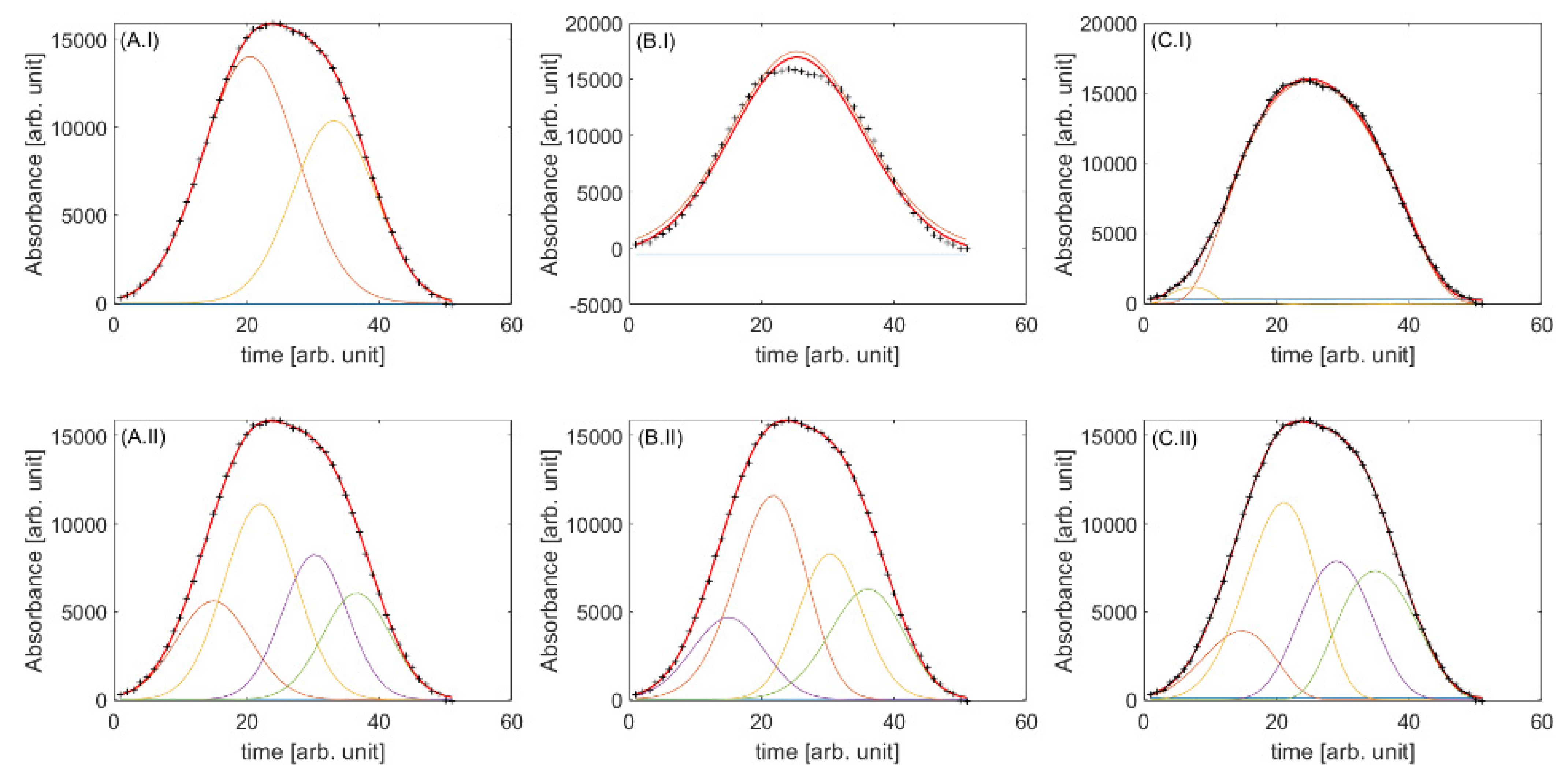
D1nh was used to compare first and second-order iterative peak fitting. For first order, the intensities from all channels were averaged. The Simplex method (fminsearch) was used to optimize the fitting parameters. The iterative process was stopped when adding an additional peak does not decrease the MSSR by more than 5% compared to the previous iteration. Results are presented in Figure 2.
With first-order data, convergence was obtained with two peaks with a Gaussian model (Figure 2A.I), one peak with a PMG1 model (Figure 2B.I) or two peaks with the PMG2 model (C.I). While proper fitting of the experimental profile can be observed in all cases, the four expected components were not mathematically separated. It was not the case when using the second-order data. Independently of the function used, similar results were obtained, with the four components separated. Slightly better results were obtained with PMG2 (Figure 2C.II, MSSR of 648), followed by PMG1 (Figure 2B.II, MSSR of 654) and Gaussian models (Figure 2A.II, MSSR of 656). However, the computation time varied from 9.5, 37.8 and 85.7 s for Gaussian, PMG and PMG2 models, respectively. It should be emphasized that first-order peak fitting is highly dependent on the channels. When selecting specific channels rather than averaging the signals, different results (including number of peaks) were obtained in Figure 2, A.I–C.I. Second-order peak fitting, provide robust deconvolution as the optimization involve all channels.
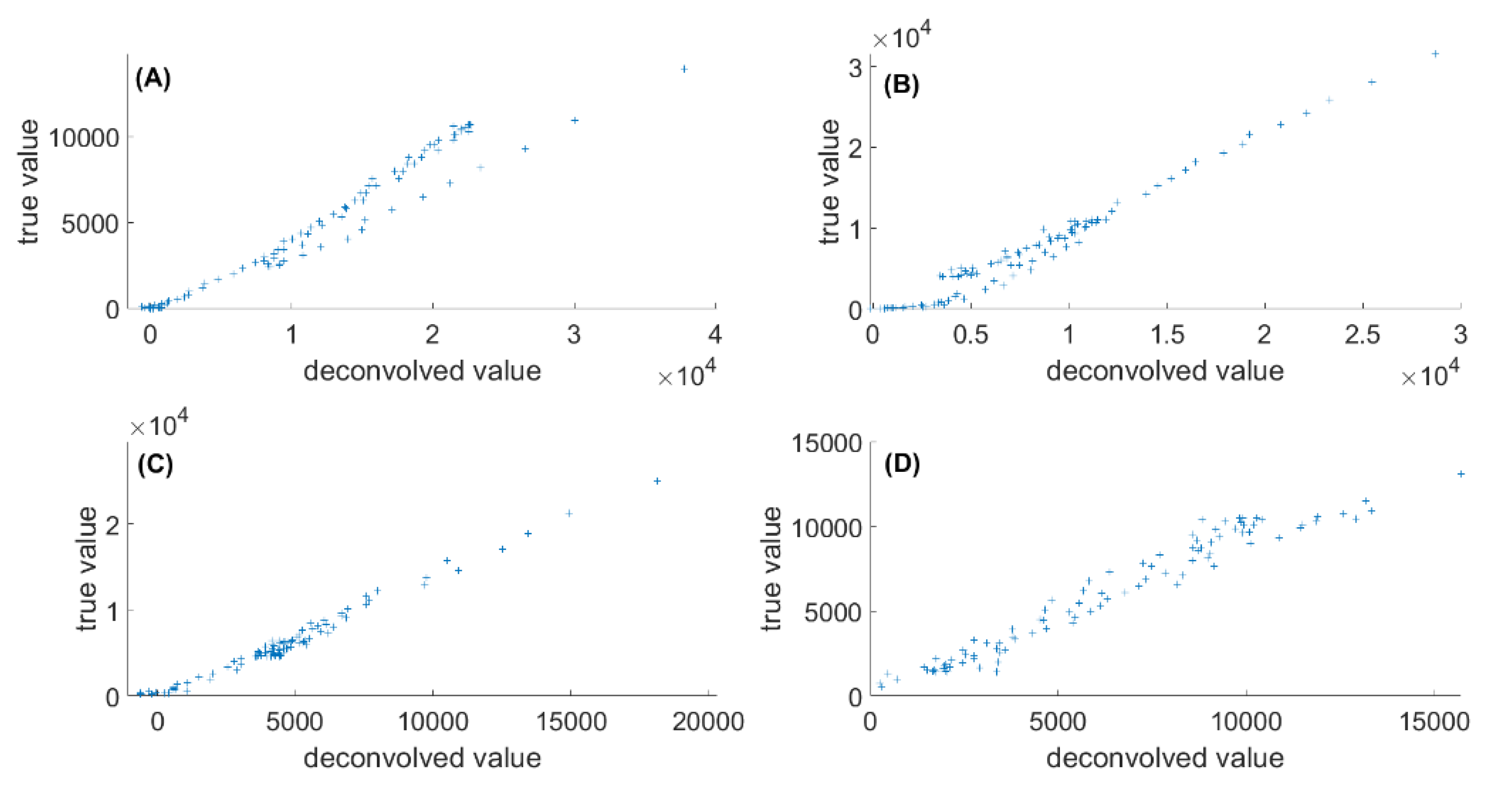
The true vs. deconvolved intensities at every channel for the four components after iterative fitting are presented in Figure 3. Good agreement was obtained with r2 of 0.950, 0.972, 0.977 and 0.951 for component 1 (Figure 3A), 2 (Figure 3B), 3 (Figure 3C) and 4 (Figure 3D) respectively.
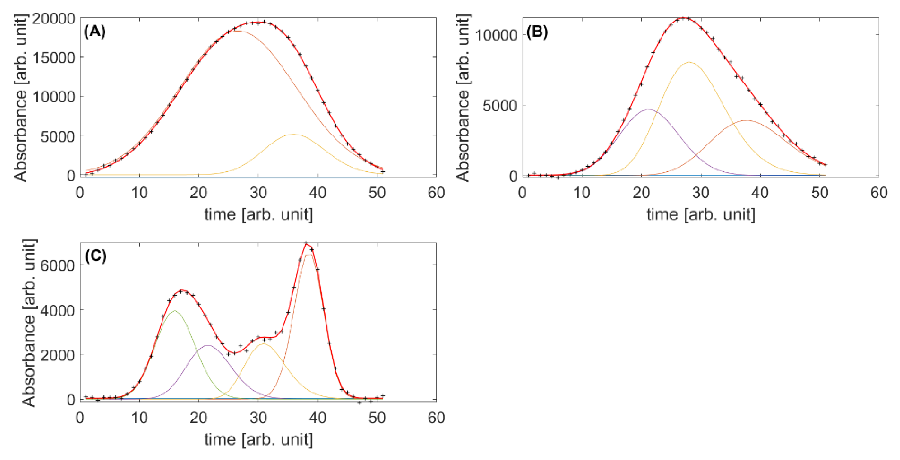
The iterative multivariate peak fitting (itMPF) was then used, with the PMG1 function, with the other three datasets. The results can be seen in Figure 4.
While the four components in D2nh (Figure 4A) and D3nh (Figure 4B) were not mathematically separated, itMPF was successful with D4nh (Figure 4C). Moreover, better agreements were obtained than with D1nh between measured and true intensities (r2 of 0.989, 0.973, 0.970 and 0.984, respectively).

2.3. Validation with HPLC-DAD Separation of Diterpene in Coffee

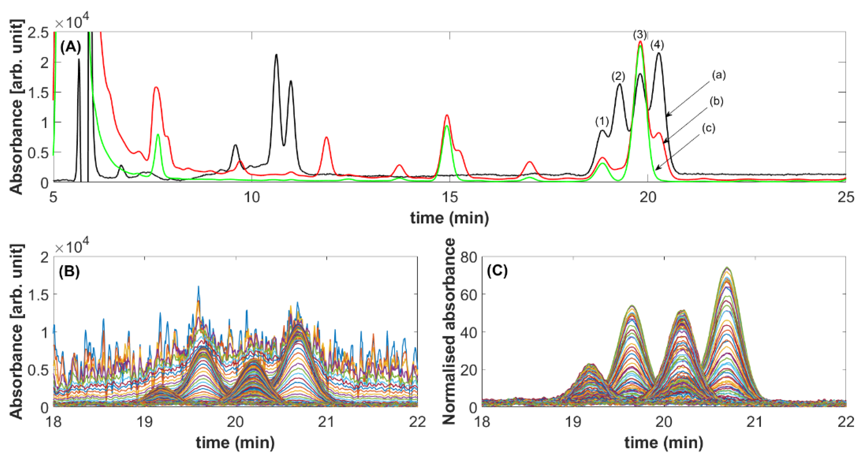
The peak fitting approach was applied to the simultaneous analysis of diterpene esters in coffee by HPLC-DAD. Typical separations are presented in Figure 5A, with, in black (a) the separation of a standard mixture of (1) kahweol oleate, (2) cafestol oleate, (3) kahweol palmitate and (4) cafestol palmitate. The profile is obtained by averaging the intensity of all wavelengths. The profiles in red (b) and green (c) correspond to the separation of a coffee sample obtained either by averaging the intensities at all wavelengths (b: 200–400 nm) or using a range selective to kahweol esters (c: 286–294 nm).
ItMPF was first used with standard mixtures of the four esters. The superposition of the profile at each wavelength is presented in Figure 5B. As a significant fluctuation of noise can be observed [30], data were normalized by the noise, estimated as the standard deviation, measured between 18 and 18.5 min of the lowest concentrated standard (Figure 5C).
The four peaks between 18 and 22 min in the standards were separated using itMPF with the PMG1 function. The ability of the software to measure the area correctly was assessed by the figures of merits (FOM) of the linear calibration. Those can be compared in Table 1 using fminsearch (simplex method) and fminnunc (quasi-Newton method) optimization algorithm. As a reference, the kahweol oleate and palmitate were quantified free of cafestol esters interferences by using the wavelength range 290 ± 4 nm [18,31] (see Figure 5A (c). Peak areas were measured using the trapezoid rule [32].
While the best results for KO and KP were obtained using classical approaches, itMPF gave good results for quantifying the four diterpene esters is with an average resolution between peaks of 0.83 (min 0.77, max 0.92). With those data, slightly better results were obtained using the fminnunc optimization algorithm.
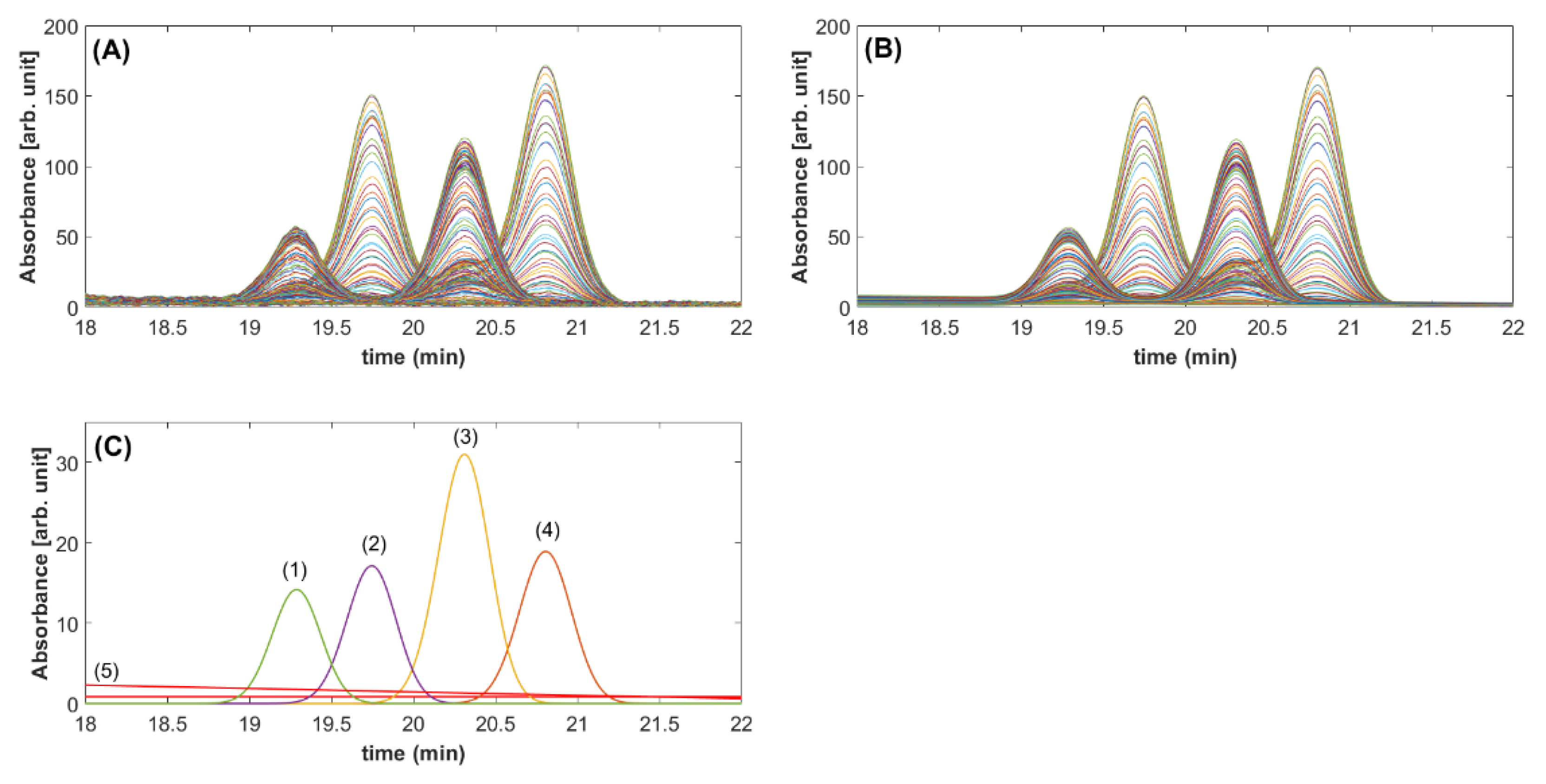
It should be emphasized that at low concentrations, more than four components are obtained. Additional components are used to better fit the baseline drift. Such an example can be seen in Figure 6. In panel A, the real data is presented with the superposition of the profile and each wavelength. Panel B shows the superposition of the fitted channels, and panel C shows the peak profiles extracted by itMPF to model the experimental data. While peaks 1 to 4 correspond to the four expected diterpene esters, an extra peak is obtained to describe the baseline better. This peak can easily be recognized due to its substantial peak variance (760 min2 vs. 0.023 ± 0.001 (n = 4) min2 for peaks 1 to 4).

3. Discussion

Iterative multivariate peak fitting is an attractive alternative to other multivariate approaches for chromatographic data. It is relevant because the number of components does not need to be known and allows quantifying individual peaks event with resolution as low as 0.5. However, the minimal resolution for good accuracy will depend on the relative intensity of the different signals and the variation of intensity along the extra dimension. While fminnunc seems to offer slightly better performance than fminsearch as optimization algorithms, computing time is a key issue. itMPF is fast when few peaks are fitted to the signals (less than 1 min for three components or less) but become slow when a higher number of peaks is used. For example, the algorithm took more than 40 min to optimize the fitting of nine peaks with a PMG1 function using the data from coffee samples. The complexity and number of fitting parameters also have a strong influence. With a Gaussian function, minimal MSSR was reached after 8 min with nine peaks. Nevertheless, this approach could be used to entire chromatograms by splitting the signals into smaller parts with few peaks.
One of the key benefits of this approach is that the number of components is automatically optimized from the data. Moreover, the baseline can be automatically detected and fitted with an extra function that must be detected and removed. The toolbox should be improved by using a more extensive set of functions.
The algorithm has been tested in multiple conditions and, most of the time, give realistic results. However, in some examples, negative peaks have been obtained. To limit their occurrence, a penalization factor for negative intensities was introduced. This factor is only used when calculating the MSSR. Constrained have also been introduced to force all peaks to have the same shape or limit the variation in peak variance within a set interval. A short tutorial is available in Appendix A.

4. Materials and Methods

4.1. Simulated Data

The simulated HPLC-DAD non-trilinear data sets were obtained from [33]. The four matrices were used (D1nh, D2nh, D3nh and D4nh). Each matrix has been generated as Di = ci·s + noise where ci (51 × 4) is the matrix of profiles (four peaks, with different positions and shapes in each dataset), s is the matrix of spectra (4 × 96) corresponding to each peak (s is the same in all datasets) and noise is the noise.

4.2. Real Data

Real data come from a published work measuring kahweol oleate, cafestol oleate, kahweol palmitate and cafestol palmitate in coffee brew [18,31]. Briefly, coffee brews were extracted using 5 mL of diethyl ether. The mixture was vortexed for 2 min, and after centrifugation, the upper phase was transferred to a clean test tube. Next, the aqueous solution was re-extracted using diethyl ether, and the combined ether phase was washed with 5 mL of 2 M NaCl solution followed by centrifugation (4000 rpm, 10 min. Finally, the clean ether phase was dried under an azote stream. Samples were kept at −22 °C until analysis using LC–DAD. Separation was achieved using a Purospher STAR LichroCART RP 18 end-capped (250 × 4 mm, 5 µm) column attached. Before injection, the dried extract was dissolved in 2.5 mL of acetonitrile and filtered through 0.45 µm filter membrane (PTFE, VWR, Radnor, PA, USA). Twenty microliters of sample were injected, and the separation was achieved using isocratic conditions for 35 min with the mobile phase made of acetonitrile/isopropanol (70:30, v/v) and pumped at 0.4 mL/min. A diode array detector, in the range of 200–400 nm, was used. After each run, the acquisition software exported data as a comma-separated-values format (EZChrom Elite 3.1.6).
For the calibration curves, mixtures of the four diterpenes esters at similar concentrations were used in the range of 2 to 200 mg/L. Eight samples were prepared and run in duplicates. All data used in this work are available in the Zenodo repository (https://zenodo.org/record/5412345).

4.3. Programming and Software

MATLAB R2020a (Mathworks, Natick, Massachusetts, USA) was used for this work; functions were programmed and run using a PC equipped with an Intel Core i7 CPU (2.80 GHz) and 18.0 GB RAM. The functions fminsearch [27] and fminunc [29] from the optimization toolbox were used. The functions IterativeMethod1_fminsearch and IterativeMethod1_fminunc were designed for this work and are available free of charge in the GitHub repository: https://github.com/glerny/itMPF [34].

Author Contributions

Conceptualization, G.L.E.; methodology, G.L.E., A.A. and M.M.; software, G.L.E.; validation, G.L.E. and M.M.; formal analysis, M.M.; investigation, M.M.; resources, A.A.; data curation, M.M.; writing—original draft preparation, G.L.E.; writing—review and editing, G.L.E., A.A. and M.M.; visualization, G.L.E.; supervision, A.A.; project administration, A.A.; funding acquisition, A.A. All authors have read and agreed to the published version of the manuscript.

Funding

This work was financially supported by: (i) Base Funding—UIDB/00511/2020 of the Laboratory for Process Engineering, Environment, Biotechnology and Energy—LEPABE—funded by national funds through the FCT/MCTES (PIDDAC); (ii) Project POCI-01-0145-FEDER-029702, funded by FEDER funds through COMPETE2020—Programa Operacional Competitividade e Internacionalização (POCI) and by national funds (PIDDAC) through FCT/MCTES.

Data Availability Statement

Data are available in Zenodo (doi:10.5281/zenodo.5412345), Matlab function are available in GitHub (https://github.com/glerny/itMPF) [34].

Conflicts of Interest

The authors declare no conflict of interest.

Appendix A

The toolbox should be downloaded from GitHub (https://github.com/glerny/itMPF) or MathWorks (https://www.mathworks.com/matlabcentral/fileexchange/97217-itmpf). The path of the downloaded files and folders should be added to the Mathlab path.
Both functions IterativeMethod1_fminunc and IterativeMethod1_fmin search use the same input and output parameters:
[Model, FittedChannels, Stats, myModel, Options] = IterativeMethod1_fminsearch (AxisX, Data, Options)
AxisX is a [nx1] vector that is the time axis, Data in a [nxm] matrix (m ≥ 1) with the first or second-order data. Options is a structure with the following information:
  • Options.maxPeaks = 20; Termination condition for the number of peaks. If Options.maxPeaks is obtained, the function stops.
  • Options.Function = ‘PMG1’; Mathematical function to be used (‘Gauss’, ‘PMG1’ or ‘PMG2’).
  • Options.LoopMe = 5; Number of times fminserach or fminunc can be repeated until convergence is reached.
  • Options.RecursiveLoop = 0.95; Termination condition for the MSSR, the algorithm will stop if MSSRn > Options.RecursiveLoop* if MSSRn-1, where MSSRn is the mean sum squared residuals obtained with n peaks after optimization.
  • Options.InitialFactor = [1 0.7 0.4]; Multiplicative factor for the initial peak shape before minimization. If Options.InitialFactor is not a single value, all values will be tested.
  • Options.MinResolution = 0; Termination condition. If two peaks have a resolution lower than Options.MinResolution, the function stops.
  • Options.Penalisation = true; If Options. Penalization is true, a penalization factor for negative intensities is used before calculating the MSSR.
  • Options.PenalisationWeight = 1.5; Penalisation factor.
  • Options.Constrained.SharedParameters = ‘None’; Constrain on the peak shape: ‘None’, ‘Partial’ or ‘Full’. If ‘None’ peak shapes are independ from each other, if ‘Full’ all peak shapes are the same, if ‘Partial’ peaks variance will fluctuate with a range set by Options.Constrained.Limits.
  • Options.Constrained.Limits = 1.5; Should be superior at 1, only used if Options.Constrained.SharedParameters = ‘Partial’.
  • Options.PointsPerPeaks = [25 75]; the average number of points per peak, used to smooth the residual when adding a new peak and avoid spikes. More than one value can be used to induce variations in the position of the new peaks and avoid local minima.
  • Options.MinMax = 0.05; Termination condition. If the maximum intensity of any peak is lower than Options.MinMax time the intensity of the most intense peak the function stops.
  • Options.Robust = false; If this option is used, an additional peak will still be tested when a termination condition is true. If with additional peaks the termination is not true anymore, the algorithms will continue.
In output, four elements are obtained:
  • Model.Peaks is a structure that contain the name of the mathematical function, the fitting parameters, the intensity at each channel and the baseline intensity.
  • FittedChannels is a [mxkxn] matrix with the intensity as a function of time for each element.
  • Stats is a structure with the Options used, the computing time, the number of peaks separated, the end conditions and the means sum square residual.
  • myModel is a [mxk] matrix with the normalized peaks model.

References

  1. Vessman, J.; Stefan, R.I.; van Staden, J.F.; Danzer, K.; Lindner, W.; Burns, D.T.; Fajgelj, A.; Müller, H. Selectivity in analytical chemistry (IUPAC Recommendations 2001). Pure Appl. Chem. 2001, 73, 1381–1386. [Google Scholar] [CrossRef]
  2. Dyson, N.; Green, J.D. Chromatographic Integration Methods; RSC Chromatography Monographs; Royal Society of Chemistry: Cambridge, UK, 1991; Volume 249, ISBN 978-0-85404-510-5. [Google Scholar]
  3. Barth, H.G. Chromatography Fundamentals, Part VIII: The Meaning and Significance of Chromatographic Resolution. LCGC N. Am. 2019, 37, 824–828. [Google Scholar]
  4. Chen, Y.; Zou, C.; Bin, J.; Yang, M.; Kang, C. Multilinear mathematical separation in chromatography. Separations 2021, 8, 31. [Google Scholar] [CrossRef]
  5. Wahab, M.F.; Hellinghausen, G.; Armstrong, D.W. The Progress Made in Peak Processing. LC GC Eur. 2019, 32, 22–28. [Google Scholar]
  6. Romanenko, S.V.; Stromberg, A.G.; Pushkareva, T.N. Modeling of analytical peaks: Peaks properties and basic peak functions. Anal. Chim. Acta 2006, 580, 99–106. [Google Scholar] [CrossRef]
  7. Caballero, R.D.; García-Alvarez-Coque, M.C.; Baeza-Baeza, J.J. Parabolic-Lorentzian modified Gaussian model for describing and deconvolving chromatographic peaks. J. Chromatogr. A 2002, 954, 59–76. [Google Scholar] [CrossRef]
  8. Purushothaman, S.; Ayet San Andrés, S.; Bergmann, J.; Dickel, T.; Ebert, J.; Geissel, H.; Hornung, C.; Plaß, W.R.; Rappold, C.; Scheidenberger, C.; et al. Hyper-EMG: A new probability distribution function composed of Exponentially Modified Gaussian distributions to analyze asymmetric peak shapes in high-resolution time-of-flight mass spectrometry. Int. J. Mass Spectrom. 2017, 421, 245–254. [Google Scholar] [CrossRef]
  9. Di Marco, V.B.; Bombi, G.G. Mathematical functions for the representation of chromatographic peaks. J. Chromatogr. A 2001, 931, 1–30. [Google Scholar] [CrossRef]
  10. Harris, D.C. Nonlinear Least-Squares Curve Fitting with Microsoft Excel Solver. J. Chem. Educ. 1998, 75, 119. [Google Scholar] [CrossRef]
  11. Erny, G.L.; Bergström, E.T.; Goodall, D.M.; Grieb, S. Predicting Peak Shape in Capillary Zone Electrophoresis: A Generic Approach to Parametrizing Peaks Using the Haarhoff−Van der Linde (HVL) Function. Anal. Chem. 2001, 73, 4862–4872. [Google Scholar] [CrossRef]
  12. Phillips, M.L.; White, R.L. Dependence of Chromatogram Peak Areas Obtained by Curve-Fitting on the Choice of Peak Shape Function. J. Chromatogr. Sci. 1997, 35, 75–81. [Google Scholar] [CrossRef] [Green Version]
  13. Li, J. Comparison of the capability of peak functions in describing real chromatographic peaks. J. Chromatogr. A 2002, 952, 63–70. [Google Scholar] [CrossRef]
  14. Vemi, A. Testing the capability of a polynomial-modified gaussian model in the description and simulation of chromatographic peaks of amlodipine and its impurity in ion-interaction chromatography. J. Sep. Sci. 2014, 37, 1797–1804. [Google Scholar] [CrossRef]
  15. Wahab, M.F.; O’Haver, T.C.; Gritti, F.; Hellinghausen, G.; Armstrong, D.W. Increasing chromatographic resolution of analytical signals using derivative enhancement approach. Talanta 2019, 192, 492–499. [Google Scholar] [CrossRef]
  16. Wahab, M.F.; Berthod, A.; Armstrong, D.W. Extending the power transform approach for recovering areas of overlapping peaks. J. Sep. Sci. 2019, 42, 3604–3610. [Google Scholar] [CrossRef] [PubMed]
  17. Dasgupta, P.K.; Chen, Y.; Serrano, C.A.; Guiochon, G.; Liu, H.; Fairchild, J.N.; Shalliker, R.A. Black Box Linearization for Greater Linear Dynamic Range: The Effect of Power Transforms on the Representation of Data. Anal. Chem. 2010, 82, 10143–10150. [Google Scholar] [CrossRef] [PubMed]
  18. Erny, G.L.; Moeenfard, M.; Alves, A. Liquid chromatography with diode array detection combined with spectral deconvolution for the analysis of some diterpene esters in Arabica coffee brew. J. Sep. Sci. 2015, 38, 612–620. [Google Scholar] [CrossRef] [Green Version]
  19. Ahmadi, G.; Tauler, R.; Abdollahi, H. Multivariate calibration of first-order data with the correlation constrained MCR-ALS method. Chemom. Intell. Lab. Syst. 2015, 142, 143–150. [Google Scholar] [CrossRef]
  20. Ruckebusch, C.; Blanchet, L. Multivariate curve resolution: A review of advanced and tailored applications and challenges. Anal. Chim. Acta 2013, 765, 28–36. [Google Scholar] [CrossRef]
  21. De Juan, A.; Vander Heyden, Y.; Tauler, R.; Massart, D.L. Assessment of new constraints applied to the alternating least squares method. Anal. Chim. Acta 1997, 346, 307–318. [Google Scholar] [CrossRef]
  22. Monago-Maraña, O.; Pérez, R.L.; Escandar, G.M.; Muñoz De La Peña, A.; Galeano-Díaz, T. Combination of Liquid Chromatography with Multivariate Curve Resolution-Alternating Least-Squares (MCR-ALS) in the Quantitation of Polycyclic Aromatic Hydrocarbons Present in Paprika Samples. J. Agric. Food Chem. 2016, 64, 8254–8262. [Google Scholar] [CrossRef] [PubMed] [Green Version]
  23. Torres-Lapasió, J.R.; Baeza-Baeza, J.J.; García-Alvarez-Coque, M.C. A Model for the Description, Simulation, and Deconvolution of Skewed Chromatographic Peaks. Anal. Chem. 1997, 69, 3822–3831. [Google Scholar] [CrossRef]
  24. Boqué, R.; Ferré, J. Using second-order data in chromatographic analysis. LC GC Eur. 2004, 17, 402–407. [Google Scholar]
  25. Nikitas, P.; Pappa-Louisi, A.; Papageorgiou, A. On the equations describing chromatographic peaks and the problem of the deconvolution of overlapped peaks. J. Chromatogr. A 2001, 912, 13–29. [Google Scholar] [CrossRef]
  26. Shanno, D.F. Conditioning of Quasi-Newton Methods for Function Minimization. Math. Comput. 1970, 24, 647. [Google Scholar] [CrossRef]
  27. Find Minimum of Unconstrained Multivariable Function Using Derivative-Free Method—MATLAB Fminsearch. Available online: https://www.mathworks.com/help/matlab/ref/fminsearch.html (accessed on 30 July 2021).
  28. Lagarias, J.C.; Reeds, J.A.; Wright, M.H.; Wright, P.E. Convergence Properties of the Nelder--Mead Simplex Method in Low Dimensions. SIAM J. Optim. 1998, 9, 112–147. [Google Scholar] [CrossRef] [Green Version]
  29. Find Minimum of Unconstrained Multivariable Function—MATLAB Fminunc. Available online: https://www.mathworks.com/help/optim/ug/fminunc.html (accessed on 30 July 2021).
  30. Erny, G.L.; Calisto, V.; Esteves, V.I. Noise normalisation in capillary electrophoresis using a diode array detector. J. Sep. Sci. 2011, 34, 1703–1707. [Google Scholar] [CrossRef]
  31. Moeenfard, M.; Erny, G.L.; Alves, A. Determination of diterpene esters in green and roasted coffees using direct ultrasound assisted extraction and HPLC–DAD combined with spectral deconvolution. J. Food Meas. Charact. 2020, 14, 1451–1460. [Google Scholar] [CrossRef]
  32. Misra, S.; Wahab, M.F.; Patel, D.C.; Armstrong, D.W. The utility of statistical moments in chromatography using trapezoidal and Simpson’s rules of peak integration. J. Sep. Sci. 2019, 42, 1644–1657. [Google Scholar] [CrossRef] [PubMed]
  33. Multivariate Curve Resolution Homepage. Available online: http://www.mcrals.info/ (accessed on 28 July 2021).
  34. Erny, G. glerny/itMPF: Iterative Multivariate Peak Fitting v1.0; Zenodo: Geneva, Switzerland, 2021. [Google Scholar] [CrossRef]
Figure 1. Simulated HPLC-DAD datasets: (A,C,E,G) superposition of the signals from all channels for D1nh, D2nh, D3nh and D4nh, respectively; (B,D,F,H) profiles for each component for D1nh, D2nh, D3nh and D4nh, respectively. Refer to the Materials and Methods section for additional information.
Separations 08 00178 g001
Figure 2. D1nh experimental data (black crosses), fitted signals (red lines) and deconvolved components using the iterative multivariate peak fitting approach: (A.I,B.I,C.I) first-order data (mean profile) fitted with a Gaussian, PMG1 and PMG2 mathematical functions. (A.II,B.II,C.II) second-order data fitted with a Gaussian, PMG1 and PMG2 mathematical functions.
Separations 08 00178 g002
Figure 3. True vs. deconvolved intensities at every channel obtained after itMPF of the D1nh dataset, with (AD) plots of the true vs. deconvolved values for the first, second, third and fourth component in D1nh dataset respectively.
Separations 08 00178 g003
Figure 4. Deconvolution of the four components by itMPF with (A) D2nh, (B) D3nh and (C) D4nh.
Separations 08 00178 g004
Figure 5. (A) Typical chromatograms; (a) standard mixture, (b) coffee analyzed using the full wavelength range, (c) coffee analyzed at 290 ± 4 nm; (1) kahweol oleate, (2) cafestol oleate, (3) kahweol palmitate and (4) cafestol palmitate. (B) Superposition of all channels corresponding to the target compounds between 18 and 22 min. (C) noise normalized intensities.
Separations 08 00178 g005
Figure 6. (A) experimental data, (B) fitted data and (C) model peaks obtained with itMPF. All diterpene esters were injected at 5 mg/mL. (1) Kahweol oleate, (2) cafestol oleate, (3) kahweol palmitate, (4) cafestol palmitate and (5) additional peak to better describe the baseline drift.
Separations 08 00178 g006
Table 1. Figures of merits (FOM) of the calibration curves using (A) itMPF with fminsearch used as optimization algorithms, (B) itMPF with fminnunc used as optimization algorithms, (C) classical approach with detection at 290 ± 4 nm. Standards were made by mixing the four diterpenes at different concentrations.
MethodFOMKO 2CO 3KP 4CP 5
Ar20.999900.999910.999970.99980
LOQ1 (mg/L)5.55.03.87.6
Br20.999790.999910.999960.99972
LOQ (mg/L)7.75.05.08.9
Cr20.99995NA0.99998NA
LOQ (mg/L)3.7NA3.1NA
1 Limit of quantification, calculated at ten times σy/x. 2 KO, kahweol oleate; 3 CO, cafestol oleate; 4 KP, kahweol palmitate; 5 CP, cafestol palmitate.
Publisher’s Note: MDPI stays neutral with regard to jurisdictional claims in published maps and institutional affiliations.