Abstract
Centrifugal Partition Chromatography is a type of Liquid-Liquid Chromatography that offers several advantages compared to Liquid Chromatography. Two immiscible liquids are utilized, and one phase has to be immobilized to implement chromatographic separation. This is performed with the help of centrifugal force. As this immobilization is not ideal, the stationary phase continuously leaks out of the apparatus (so-called bleeding). We measured the stationary phase’s loss precisely and implemented a controller to compensate for it during operation. This innovative mode of operation is called redosing of the stationary phase and prolongs the experimental runtime significantly. In a first step, we implemented an open-loop controller, which was capable of counteracting bleeding but could not dial to a given setpoint precisely. Therefore, a closed-loop controller with a moving frame shifting factor was programmed. This controller reached and maintained setpoints with high accuracy. The last experimental step was to check for boundaries of this new degree of freedom. In addition, we highlighted the accompanying hydrodynamics during redosing with the help of Computational Fluid Dynamics. We were able to show the influence of different volumes of the redosed stationary phase on the flow regime.
1. Introduction
In Centrifugal Partition Chromatography (CPC), no solid stationary phase is used. Instead, immiscible two liquid phases are utilized as stationary and mobile phases. The immobilization of the stationary phase is achieved with the help of centrifugal force: The fluid is entrapped inside the chambers and interconnecting channels of a spinning rotor [1]. Then, it is possible to pump the mobile phase through the immobilized stationary phase. The former is dispersed at every chamber’s inlet before the mobile phase coalesces at the chamber’s outlet [2]. The retention factor Sf* indicates the stationary phase left in the system.
It is well-known from the literature that, in this context, there is an effect called bleeding: Droplets of the stationary phase are carried out of the rotor because of an imperfect coalescence zone inside the chambers [3,4]. This lowers the amount of stationary phase left in the apparatus over time. Furthermore, bleeding starts next to the inlet of the rotor and progresses towards the outlet of the mobile phase over time, as we were able to show in a previous publication [5]. Consequently, the separation efficiency over time is not constant but decreases. On the contrary, a high chromatographic resolution ensures high purities, especially when dealing with complex separation tasks like isolating the antioxidant astaxanthin, flavonoids, or even proteins like myoglobin or lysozyme [6,7,8,9,10,11]. When operated in the classic “batch-to-batch” mode, the number of separation cycles and, therefore, the productivity are limited due to the loss of the stationary phase mentioned.
This challenge can be addressed in two ways: first of all, via the adaptation of the apparatus itself. With the help of sequential Centrifugal Partition Chromatography, a continuous feed implementation can be realized, significantly impacting productivity [12,13,14,15,16]. Another option is Continuous Centrifugal Extraction, where the liquid phases and feed are continuously added [17,18]. Hence, bleeding can be counteracted, optimizing productivity, too.
On the downside, both solutions require significant technical effort for implementation and have a complex operation. For these reasons, this work focuses on a second conceivable solution. With the help of an adapted operating mode of a standard Centrifugal Partition Chromatograph, bleeding could be addressed. The goal is to prove whether the stationary phase’s loss over time could be counteracted with the help of redosing the stationary phase during operation. This solution implies several advantages: with a constant amount of stationary phase left in the rotor over time, the chromatographic resolution should be constant, too. Therefore, high productivity would be ensured. Furthermore, the instrumental expenditure and costs are comparatively low, as only valves and software solutions are necessary.
In addition to the benefits mentioned, operating the apparatus with a constant amount of stationary phase immobilized in the rotor implies another advantage: with the system’s retention, a new degree of freedom is introduced. Then, separation tasks could be performed with constant (as mentioned) but adjustable retention values. In analogy to Liquid Chromatography, this would be equivalent to changing the length of a column during operation. To conclude, the main questions to be addressed in this paper are:
- Hydrodynamics during redosing. Disturbances during operation should be as confined as possible to not impact the separation task. With Computational Fluid Dynamics (CFD), flow regimes during the redosing of the stationary phase become investigable. Therefore, the simulation of redosing is a suitable tool for gaining knowledge about the hydrodynamics involved.
- Redosing: Experimental validation as a proof of concept. With the help of an adapted experimental setup with corresponding software implementation, the progression of retention factors over time will be investigated. Therefore, several variables must be defined: the volume of the redosed stationary phase, the interval of redosing, and the interval of retention measurements. Furthermore, a robust, precise, and reliable control system is a crucial target.
2. Materials and Methods
2.1. Computational Fluid Dynamics: Simulation of Redosing
To simulate the hydrodynamics during the redosing of the stationary phase, the Computational Fluid Dynamics (CFD) model established in our previous publication was adapted [19,20]. A retention value (Sf) of 0.5 was chosen as the initial condition for the simulation of redosing during operation. The behavior of the chambers during redosing was simulated at different volumes of the redosed stationary phase to investigate the general feasibility of the redosing concept. The simulation aimed to evaluate the effect of the stationary phase addition on the chambers’ hydrodynamics. The total volume redosed was varied between 0.3 × Vchamber and 1 × Vchamber (0.155 mL). With the volumes selected, it was thus possible to investigate the replenishment of the stationary phase in the chambers. Initially, the ducts were assumed to be filled with mobile phase [4]. The inflow velocity of both phases was set to be constant, being = 0.15 m·s−1. The phase fraction at the inlet is time-dependent depending on which of the two phases is the inflowing one. The different volumes of the redosed stationary phase were implemented by varying the redosing times because the volume flow was set to be constant and equal to the volume flow of the mobile phase. After 0.5 s of initial feeding with the mobile phase, the stationary phase was redosed up to 1.24 s, until the switch back to the mobile phase was executed. The simulations were finished after a total time of 2 s.
2.2. Centrifugal Partition Chromatograph
All experiments were performed utilizing a Centrifugal Partition Chromatograph provided by Chromaton (FCPC, Chromaton, Annonay, France). A single-disc rotor with six transparent areas (viewing windows) was used, as already described in the literature [4,5]. A detailed figure is given in Figure A1. The rotor has a total volume of 10.4 mL; the chamber geometry was the same as the FCPC-type (Sfmax = 0.782), also purchased from Chromaton. We used a LED flash (wavelength 627 nm, type CCS TH 63X60RD from Stemmer Imaging, Puchheim, Germany) and a camera (AccuPIXEL© TM 1327GE from Jai Pulnix, Yokohama, Japan), to enable video recording of the viewing windows during operation. The last part of the setup was two pumps (Azura P2.1S, Knauer, Berlin, Germany) for the mobile and stationary phase and a valve (93967, Knauer, Berlin, Germany) to switch between phase flows. A schematic representation of the experimental setup is given in Figure 1. The volumetric flow rate of both the stationary and mobile phase was 15 mL⋅min−1. This flow rate was chosen according to the flow regime analysis performed previously. Thereby, a highly dispersed flow regime was ensured [5].
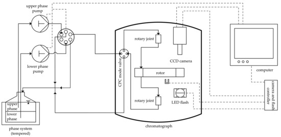
Figure 1.
Schematic representation of the experimental setup. Fluid flow is indicated in solid lines. Data signals are marked in dashed lines.
2.3. Phase System
The phase systems used were from the Arizona family, containing heptane (99.8%), methanol (99%), ethyl acetate (99.9%) (all supplied by VWR International, Radnor, PA, USA), and water purified by a MILLI-Q® system (Millipak® Express 40, Merck, Darmstadt, Germany) [21,22]. All fluids were used within 24 h after initial preparation to avoid hydrolysis [23]. Both liquid phases stayed in contact during the experiments, maintaining a thermodynamic equilibrated state. Methylene blue (20 mg/L of heavy phase, Merck, Darmstadt, Germany) was added to amplify the contrast between both phases. This dye stains the aqueous phase in blue (not affecting hydrodynamics).
2.4. Redosing Experiments
To calculate the stationary phase necessary to compensate for bleeding, we measured the initial retention factor and the Sf* after 20 min (Figure 2: preceding determination of Vstat). In a second step, the volume of the bled stationary phase was redosed repeatedly in intervals of 20 min. Analysis of raw data during the experiment is not necessary, but a downside of the program is that it cannot compensate for differences in bleeding rate. These experiments are called open-loop redosing experiments. With the help of camera-based measurements, the system’s retention was measured directly before and after each redosing was executed [5,24].
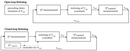
Figure 2.
Schematic sequence of open-loop and closed-loop redosing experiments.
To ensure that the measurement of Sf* after redosing was not disturbed by hydrodynamic effects caused by redosing (meaning the critical lower tctrl, at which point the temporary fluctuations in retention after redosing have subsided in each viewing window), we measured the impact of redosing on hydrodynamic stability beforehand. Therefore, the retention was measured at high resolution (10 s intervals) after initial redosing.
On the other hand, closed-loop redosing experiments imply the usage of a controller. Hence, a program was coded that could analyze each measurement’s raw videos before redosing and then calculate the redosing volume necessary to reach a predefined retention setpoint. Both redosing variants are schematically illustrated in Figure 2.
Subsequently, we implemented a moving-frame shifting factor to improve the redosing algorithm. The way in which the shifting factor should enhance the algorithm is schematically presented in Figure 3. The mean phase retention between a control measurement and the subsequent measurement before redosing should equal the setpoint since the separation occurs in this time frame. The general idea of the moving-frame shifting factor is to add a variable gain to the proportional control structure if there is an inequality. Instead of using a shifting factor, one could also change the definition of the setpoint and determine the setpoint such that an overdosing of stationary phase takes place. The overall advantage is the ability to react to the actual hydrodynamic behavior of the plant combined with a smoothening effect due to the backward-moving frame.
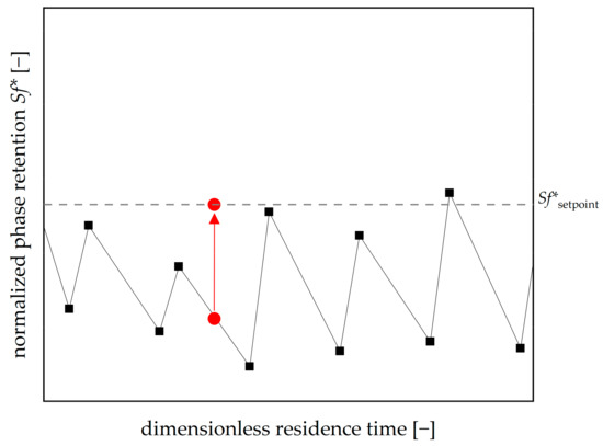
Figure 3.
Introduction of a moving-frame shifting factor to improve the control of the stationary phase retention. The goal is to align the mean retention value and the setpoint (dashed line, red dots).
The shifting factor θcalc is calculated using the formula given in Equation (3).
A moving frame is used to further improve the control, such that the applied shifting factor θcalc is the mean of the shifting factor in the prior control cycle θi-1 and the current one, as described in Equation (4).
Subsequently, the shifting factor is multiplied by Sfmax and added to the offset between the setpoint for Sf* and the current measurement. This sum is then used for the calculation of the volume to be redosed (Vstat):
The redosing experiment mentioned beforehand was repeated with the new algorithm to benchmark the performance of the optimized redosing algorithm (with movingframe shifting factor). All inputs and parameters were kept constant. An Arizona N system was prepared to determine the equilibrium retention Sf*equ; therefore, the rotor was flooded with the stationary phase. Sf*equ describes the retention value after initial disturbances in the system subsided. Subsequently, the inlet stream was switched to the mobile phase. After six rotor volumes passed, the stationary phase retention was measured for different rotational speeds and volumetric flow rates.
The setpoint was increased in minor steps to determine the upper limit of the Sf*setpoint until the mean Sf* during closed-loop redosing differed significantly from the one mentioned previously.
3. Results and Discussion
3.1. Simulation of Stationary Phase Redosing
As shown in our previous publication, a double-cell flow area represents experimental data accurately [19,25]. In particular, with the second chamber being simulated, further investigation of stationary phase bleeding over time becomes possible. To counteract the loss of fluid stationary phase from chamber one in the simulation, we developed a redosing strategy of the stationary phase as an operating mode to stabilize the retention in the CPC during operation. To stabilize the performance of the CPC, it is desirable to keep the Sf of the chambers inside the range 0.2 ≤ Sf ≤ 0.8 [26]. Furthermore, chromatographic separation must not be negatively influenced by the redosing. Thus, the redosing process should not significantly disturb the hydrodynamic equilibrium of the chambers near the inlet.
Based on the simulation of the two connected CPC chambers, the following consecutive bleeding mechanism can be deduced: The Sf in the first chamber decreases significantly faster than in the second chamber. The pure mobile phase flows into the first chamber while the second chamber’s inlet stream equals the first chamber’s outflow. This stream consists of the mobile phase and the bled stationary phase. Accordingly, the stationary phase only exits from the first chamber. In contrast, in the second chamber, this phase both exits and enters – with the inflowing stationary phase partly compensating for the bleeding in the second chamber. As soon as the first chamber of the CPC is completely filled with the mobile phase, phase separation is no longer possible in the chamber. Simultaneously, this leads to a pure mobile phase flow into the second chamber. Hence, the inlet stream no longer contains any stationary phase to compensate for the bleeding in the second chamber. As a result, the Sf of the second chamber decreases faster, analogously to the Sf of the first chamber [5,19].
Even though the first chamber of the CPC rotor cannot be observed, we were able to show that the retention of the chambers falls below a critical lower retention value one after another [5]. Based on this consecutive flooding, it can be concluded that stabilizing the Sf of the first chambers ensures stabilized retention in all following chambers of the rotor.
Figure 4 illustrates the hydrodynamics of the chambers simulated and the resulting phase fractions over time. These are defined as follows:
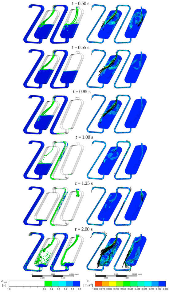
Figure 4.
Redosing of 1 × Vchamber of stationary phase. In the pictures on the left, the interphase between the mobile and the stationary phase is marked with an isosurface with = 0.5. In the images on the right, the velocity is shown on the middle cross-sectional plane of the flow area. The face velocity is 0.15 m·s−1, and the rotational speed is 1000 rpm counterclockwise. The phase system used is Arizona N.
The characteristic velocity field of the CPC chambers is formed after the initialization period of 0.5 s. After this initial period, the feed was switched from the mobile phase ( = 0) to pure stationary phase ( = 1). With the beginning inflow of the latter, the velocity field changes significantly since no mobile phase flows into the first chamber. The centrifugal force ensures that the mobile phase coalesces at the outlet of the chambers immediately. As a result, there is no dispersion of the mobile phase at the first chamber’s inlet. A vortex is formed in a clockwise direction in the pure stationary phase, as we could already show [19,27]. The stationary phase is not entrained into the coalescence zone, so the interface between the coalesced mobile and stationary phase is sharp and has a minimal surface area. The inflowing stationary phase and the vortex mentioned do not influence the course of the interface. The stationary phase neither mixes in the mobile phase nor disperses in the coalescence zone in the lower part of the chamber. Instead, the stationary phase is deflected at the interface of the coalescence zone due to the interface forces and the density differences of the two phases. This is how the vortex is created, whereby the direction of rotation is opposite to that during standard operation.
As the inflow of the stationary phase progresses, the mobile phase is further displaced from the first chamber. The interface remains sharp in that process, and only the mobile phase flows into the second chamber. As a result, the stationary phase is less entrained. Then, 0.85 s after the start of the simulation, 0.5 × Vchamber of stationary phase is added to chamber 1. Within this timespan, the Sf of the first chamber increases to 0.92. In addition, only a small amount of the mobile phase is present at the chamber’s outlet, and the stationary phase is already flowing into the channel connecting the chambers. The Sf of the second chamber is 0.48 at that point, which is lower than the simulation’s start retention. The pure mobile phase continues to flow into the second chamber at that time.
When the stationary phase flows into the second chamber (after 1 s), the velocity field changes analogously to the behavior in the first chamber. However, the inflowing volume flow in the second chamber contains small amounts of mobile phase. This effect is caused by the centrifugal force, which acts against the flow direction in the duct [28,29]. Unlike in the chambers and due to its higher density, the mobile phase is not entirely displaced by the stationary phase but is partially entrained in the second chamber. As a result, the mobile phase components are accelerated and cause turbulence at the inlet of the second chamber. Nevertheless, the sharp phase interface with the coalescence zone is maintained. From 1.25 s, the switch back to the mobile phase is performed. The Sf of the first chamber is at 0.91, and the Sf of the second chamber is at 0.76. From this timestep, the characteristic velocity field of the chambers is formed as described.
Comparing the resulting retention progression over time, different effects for different volumes of re-dosed stationary phase are apparent (Figure 5).
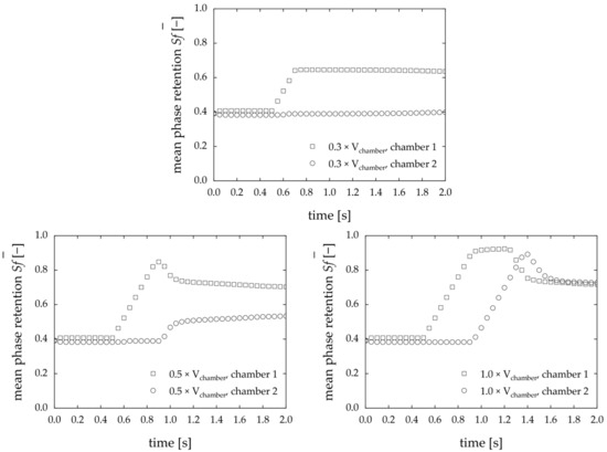
Figure 5.
Time-dependent Sf in the simulation of stationary phase redosing with varying volumes of redosed stationary phase. The face velocity is 0.15 m·s−1, and the rotational speed is 1000 rpm counterclockwise. The phase system used is Arizona N.
The less stationary phase is redosed, the less disturbance is detected in the downstream chambers—especially in the second chamber. In the first chamber, the Sf increases with the addition of stationary phase up to a global maximum. At 0.3 × Vchamber, the retention in the second chamber remains unaltered. The stationary phase does not entirely displace the mobile phase, and the coalescence zone at the chamber’s outlet is maintained, resulting in minimized bleeding from the first chamber. In analogy to Figure 4, the corresponding results for the phase fraction are shown in Figure A2.
Those simulations indicate that the redosing of the stationary phase has the potential to contribute to the CPC’s stable operation over long periods of time. The more stationary phase is redosed, the more the behavior of downstream chambers is influenced by the redosing process. Thus, the simulation results confirm the assumption that the Sf of the chambers can be kept stable if the stationary phase lost from the first chamber can be replenished. In the next step, a proof of concept is presented to validate the applicability of redosing experimentally.
3.2. Open-Loop Redosing Experiments
As mentioned, the determination of the volume of the stationary phase to be redosed during the experiments was performed initially. Therefore, the apparatus was operated without redosing, and the retention was measured in intervals of 10 min. The corresponding results are shown in Figure 6.
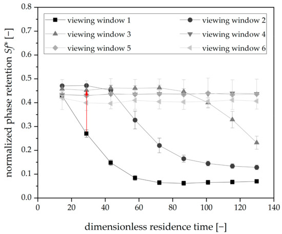
Figure 6.
Phase retention over dimensionless residence time for Arizona N, mobile phase flow: 15 mL⋅min−1, 22 °C, 750 rpm, descending mode, tripled runs. Each graph indicates the retention values of one viewing window. The red arrow highlights the redosing interval and ∆Sf* to be compensated.
The initial retention value for all viewing windows is 0.43 ± 0.06, with the Sf* rapidly decreasing in the first viewing window. The same applies to the following viewing windows but shifted timewise. This avalanche-like progression of bleeding was already described in detail [5]. In order to mitigate this phenomenon through the implementation of redosing, two variables must be specified: First, the redosing interval (tloop) and second, the volume of the stationary phase to be redosed (Vstat). The redosing interval was defined concerning the critical lower Sf of 0.2, which must be maintained to ensure a sufficient separation performance [26,30]. In the first viewing window, the first retention value lower than the limit mentioned was measured after 30 min (43 dimensionless residence times). Therefore, 20 min (28.4 dimensionless residence times) was chosen as the redosing interval.
In the next step, Vstat has to be defined: the volume of stationary phase necessary to compensate for bleeding between 0.27 (Sf* after 28.4 dimensionless residence times) and 0.43 (initial Sf* at the same time) is 0.107 mL.
Finally, the measuring interval is needed. The CFD simulations show that the stationary phase leaks from upstream chambers into downstream chambers. Redosing promotes this effect. Hence, measurements of retention directly after redosing could imply falsely increased values for Sf*. Consequently, a timespan tctrl was defined, after which an accurate retention measurement was possible. The corresponding experimental result is shown in Figure 7.
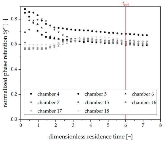
Figure 7.
Phase retention over dimensionless residence time for Arizona N after a single initial redosing event (Vstat: 0.25 mL), mobile phase flow: 15 mL⋅min−1, 22 °C, 750 rpm, descending mode, tripled runs. Retention values for the chambers of the first and second viewing windows. The red line indicates the timespan, after which the control measurement after redosing was started.
As can be seen here, the disturbance in the phase retention directly after an initial redosing step is maximal for the chambers of the first viewing window (4–7). The chambers of the second viewing window (15–18) show only minor responses to the redosing performed. After six dimensionless residence times, the disturbance has subsided. Therefore, the timespan for retention control after redosing was set to the same value.
With all of the degrees of freedom set, open-loop redosing experiments were conducted. The corresponding mean Sf* for all viewing windows for the tripled redosing runs is shown in Figure 8.
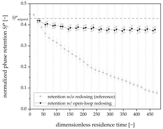
Figure 8.
Phase retention over dimensionless residence time for three open-loop redosing runs with Arizona N. Mean retention values for all viewing windows. The redosing interval is 20 min (dashed vertical red lines). Mobile phase flow: 15 mL⋅min−1, 22 °C, 750 rpm, descending mode. For reference, tripled mean phase retention values without redosing are shown in grey (corresponding to Figure 6). A dashed horizontal line indicates the Sf*setpoint.
The open-loop redosing significantly contributes to the system’s stability: the mean initial Sf* for all three runs is 0.45, and the final mean Sf* after 469 dimensionless residence times (325 min) is 0.38.
On the contrary, the reference run without redosing has a final Sf* of 0.07 while the starting Sf* was 0.45 and, therefore, comparable to the redosing runs. Regarding solvent consumption, 3.6 × 10⁻³ mL of stationary phase per dimensionless residence time was necessary to counteract bleeding in the open-loop experiments.
In conclusion, the open-loop experiments are suitable for stabilizing retention in this case. Nevertheless, further potential for optimization is evident: the bleeding rates of the redosing experiments indicate a slight retention decrease over time. Extensive iterative testing of adapted volumes of stationary phase to be redosed (Vstat) and/or redosing intervals (tloop) would be necessary to counteract this. At the same time, this optimization would only be valid for the chosen operating point for the phase system. For example, altering the volumetric flow rate would imply a new set of references and redosing experiments to determine suitable Vstat and tloop.
When focusing on the retention values for the first viewing window (chambers 4–7), another potential for optimization becomes apparent (Figure 9).
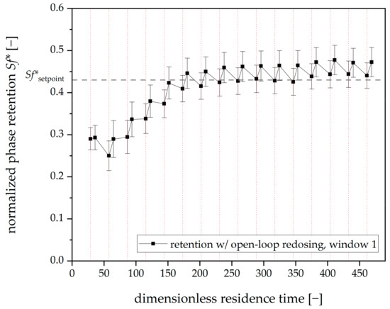
Figure 9.
Mean phase retention over dimensionless residence time for three open-loop redosing runs with Arizona N. Tripled runs. Mean retention values over the first viewing window. The redosing interval is 20 min (dashed vertical red lines). Mobile phase flow: 15 mL⋅min−1, 22 °C, 750 rpm, descending mode.
The error bars indicate that the different redosing runs (with identical settings) show different behavior. The open-loop redosing of the stationary phase could not counteract bleeding, i.e., in the first segment of the rotor. These variations might occur due to differences in hydrodynamics. With each run being performed with a renewed phase system, even slight deviations in the phase systems composition could lead to differing physical properties (i.e., ∆ρ, ∆η, γ) and, therefore, differing hydrodynamics. The latter would impact the bleeding dynamics significantly [4].
Consequently, a Centrifugal Partition Chromatography setup is needed, which can react to different bleeding dynamics by altering redosing parameters. Hence, closed-loop redosing of the stationary phase was used. The retention value was measured directly before redosing, and the setpoint for Sf* was used to control Vstat nearly online.
Therefore, the algorithm to measure the retention with the help of a camera was adapted [5,24]. With the help of the Fourier transformation, the computational effort and, consequently, the necessary duration for calculations was reduced significantly [5]. This optimization makes the image processing algorithm suitable for controlling retention parameters. In the next step, corresponding closed-loop experiments were executed.
3.3. Closed-Loop Redosing Experiments
In the following, the results of the closed-loop redosing experiments are discussed. The outcomes of the experiments are shown in Figure 10. In the first cycle (before 50 dimensionless residence times), the measured value was above the setpoint; consequently, no stationary phase was added, and the retention in the subsequent control measurement continued to decrease.
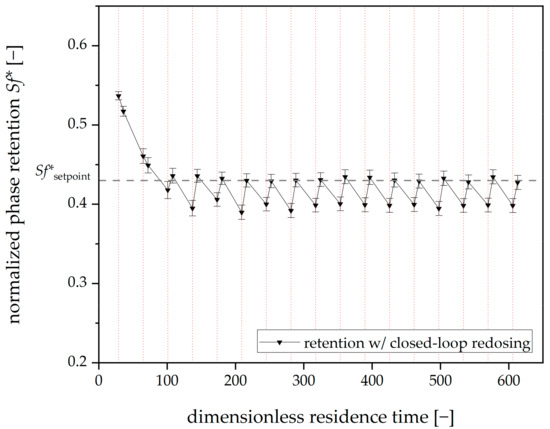
Figure 10.
Mean phase retention over dimensionless residence time for three closed-loop redosing runs (without a moving-frame shifting factor) with Arizona N. Tripled runs. Mean retention values for all viewing windows. The redosing interval is 20 min (dashed vertical red lines). Mobile phase flow: 15 mL⋅min−1, 22 °C, 750 rpm, descending mode.
From the second cycle onwards, the stationary phase is redosed in each cycle. With the automated routine developed, constant retention can be maintained, and thus, bleeding can be successfully counteracted. The mean retention in the timespan during which the stationary phase is added is Sf* = 0.41 ± 0.02, which means that the mean value is slightly below the setpoint of Sf*setpoint = 0.43. For this purpose, 0.047 ± 0.008 rotor volumes of the stationary phase were redosed per hour of operation. After a redosing step, the setpoint is usually minimally exceeded or undercut. Since a separation occurs between a control measurement and a new redosing step, it would be helpful if the average retention in this area corresponded to the setpoint. For this purpose, a moving-frame shifting factor was implemented.
The corresponding results are shown in Figure 11. The mean retention (after the first redosing event) is sf = 0.425 ± 0.03, which means that the mean value is still slightly below the setpoint. For this purpose, 0.052 ± 0.01 rotor volumes of the stationary phase were redosed per hour of operation. A comparison to the results without implementing the shifting factor shows that the redosed volume of the stationary phase is not significantly different.
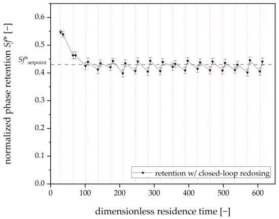
Figure 11.
Mean phase retention over dimensionless residence time for three closed-loop redosing runs with a moving-frame shifting factor (Arizona N). Tripled runs. Mean retention values for all viewing windows. The redosing interval is 20 min (dashed vertical red lines). Mobile phase flow: 15 mL⋅min−1, 22 °C, 750 rpm, descending mode.
In conclusion, redosing the stationary phase with the help of a closed-loop controller and a moving-frame shifting factor is suitable for maintaining constant retention values for the given system and operation parameters.
In the next step, the limits of the Sf*setpoint have to be determined. A lower limit can be drawn from the literature [26]. Below values of sf = 0.2, separation performance is drastically decreases. Conversely, the upper limit can be derived from experimental data: The aim is to validate the hypothesis of whether the upper limit for the Sf*setpoint is related to the retention equilibrium value Sf*equ. The latter is defined as the retention value, which is reached quasi-instantaneously after the start of each experimental run (e.g., after six dimensionless residence times). This value depends significantly on the operational parameters (volumetric flow rate, rotational speed, rotor geometry) for a given phase system. Therefore, these parameters were altered, as shown in Figure 12.
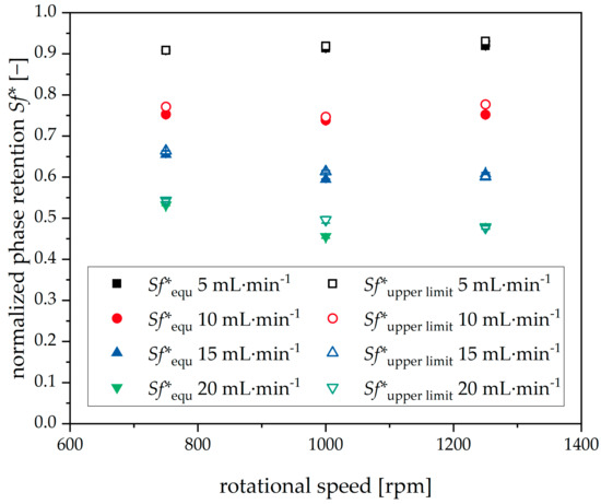
Figure 12.
Initial equilibrium phase retention Sf*equ and upper limit phase retention Sf*upper limit for closed-loop redosing for different rotational speeds and volumetric flow rates. Descending mode, 22 °C, Arizona N. Rotor with 66 chambers, tripled runs.
Furthermore, the upper limit Sf* which is reachable with the help of closed-loop redosing (Sf*upper limit) was determined experimentally. The Sf*setpoint was increased until the mean Sf* during redosing differed significantly from the given setpoint. The last Sf*setpoint in congruence with the mean Sf* is the Sf*upper limit, also shown in Figure 12.
Sf*equ decreases as the flow rate increases, indicating a linear relationship. Furthermore, the rotational speed variation has a significantly lower influence on initial phase retention, with a slightly parabolic relationship for the volume flows at 10, 15, and 20 mL·min−1. In comparison, for 5 mL·min−1, hardly any change is evident.
Sf*upper limit, on the other hand, shows a similar trend, with no significant divergence from Sf*equ. Therefore, it can be stated that, for the phase system and rotor geometry given, experimental validation of Sf*equ leads to predictability of Sf*upper limit—severely shrinking the experimental effort to determine the boundaries of Sf*setpoint.
4. Conclusions
In conclusion, redosing the stationary phase during the operation of a Centrifugal Partition Chromatograph can significantly prolong the apparatus’s runtime. In a first step, we simulated the hydrodynamics during redosing with the help of Computational Fluid Dynamics. Depending on the volume of the redosed stationary phase, the disturbances in the chambers were minor, indicating the principal suitability of the subsequent experimental implementation.
To do so, the volume of the stationary phase to be redosed also referred to as closed-loop redosing, can be calculated beforehand. This innovative mode of operation ensures constant retention values over time and, therefore, a stable operation. Based on that, it should be possible to stabilize the separation efficiency over time.
Open-loop redosing, on the other hand, is able to stabilize the retention as well, but suffers from minor drawbacks, such as increased experimental effort. In conclusion, closed-loop redosing is the optimal method to counteract bleeding. Furthermore, disturbances caused by redosing were analyzed. For the given operation point, hydrodynamics stabilized six dimensionless residence times after the addition of thestationary phase.
The Sf*setpoint is a new degree of freedom which can be used when optimizing operating points for a given separation task. Regarding hydrodynamics, the lower boundary for this variable is the need to keep at least some stationary phase immobilized to ensure chromatographic separation of the sample. Practically and according to the literature, the lower limit for the Sf to maintain sufficient separation efficiency is 0.2 [26].
For the upper limit, we prove the equality of the highest Sf*, reachable for a given setpoint, and the Sf*equ, the retention value established shortly after the start of the experiment. This insight drastically reduces the experimental effort to find the upper limit for the Sf*setpoint for the given phase system. Only single experiments are necessary to determine the upper limit of this degree of freedom for a given volumetric flow rate and rotational speed.
This new operation mode must be applied to a separation task in the next step. With the Sf*setpoint, a new variable influencing the separation is introduced which has to be optimized. We will further demonstrate this task with the help of a model system and a binary separation task.
Author Contributions
Conceptualization, F.B. and G.S.; methodology, F.B.; software, J.H., F.B. and S.V.; experimental validation, S.V., D.H., M.N., J.H. and F.B.; formal analysis, S.V., D.H., M.N., J.H. and F.B.; investigation, S.V., D.H., M.N., J.H. and F.B.; data curation, F.B.; writing—original draft preparation, F.B.; writing—review and editing, F.B. and G.S.; visualization, F.B.; supervision, G.S. All authors have read and agreed to the published version of the manuscript.
Funding
This research received no external funding.
Data Availability Statement
Data are contained within the article.
Acknowledgments
The authors gratefully acknowledge the computing time provided on the Linux HPC cluster at Technical University Dortmund (LiDO3), partially funded in the course of the Large-Scale Equipment Initiative by the German Research Foundation (DFG) as project 271512359.
Conflicts of Interest
The authors declare no conflicts of interest.
Appendix A
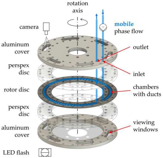
Figure A1.
Explosion view of the rotor. On the rotor disc are 66 chambers with interconnecting ducts embedded. Perspex discs with additional sealing (not shown) and aluminum covers ensure tight sealing. The six viewing windows in the aluminum cover allow visual access (camera, LED flash). The fluid flow of the mobile phase is highlighted by blue lines. The visible chambers are: chamber 4–7 (viewing window 1), chamber 15–18 (viewing window 2), chamber 26–29 (viewing window 3), chamber 37–40 (viewing window 4), chamber 48–51 (viewing window 5), chamber 59–63 (viewing window 6).
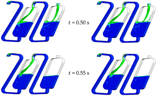
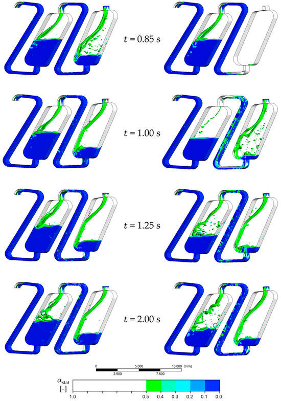
Figure A2.
Redosing of 0.3 × Vchamber (left) and 0.5 × Vchamber (right) of stationary phase. The interphase between the mobile and the stationary phase is marked with an isosurface with = 0.5. The face velocity is 0.15 m·s−1, and the rotational speed is 1000 rpm counterclockwise. The phase system used is Arizona N.
References
- Marchal, L.; Legrand, J.; Foucault, A. Centrifugal partition chromatography: A survey of its history, and our recent advances in the field. Chem. Rec. 2003, 3, 133–143. [Google Scholar] [CrossRef] [PubMed]
- Chollet, S.; Marchal, L.; Jérémy, M.; Renault, J.H.; Legrand, J.; Foucault, A. Methodology for optimally sized centrifugal partition chromatography columns. J. Chromatogr. A 2015, 1388, 174–183. [Google Scholar] [CrossRef] [PubMed]
- Van Buel, M.J.; van Halsema, F.E.D.; van der Wielen, L.A.M.; Luyben, K.C.A.M. Flow regimes in centrifugal partition chromatography. AIChE J. 1998, 44, 1356–1362. [Google Scholar] [CrossRef]
- Adelmann, S. On Hydrodynamics in Centrifugal Partition Chromatography. Ph.D. Dissertation, TU Dortmund University, Dortmund, Germany, 2014. [Google Scholar]
- Buthmann, F.; Laby, P.; Hamza, D.; Koop, J.; Schembecker, G. Spatially and Temporally Resolved Analysis of Bleeding in a Centrifugal Partition Chromatography Rotor. Separations 2024, 11, 56. [Google Scholar] [CrossRef]
- Destandau, E.; Boukhris, M.A.; Zubrzycki, S.; Akssira, M.; Rhaffari, L.E.; Elfakir, C. Centrifugal partition chromatography elution gradient for isolation of sesquiterpene lactones and flavonoids from Anvillea radiata. J. Chromatogr. B 2015, 985, 29–37. [Google Scholar] [CrossRef] [PubMed]
- Fábryová, T.; Tůmová, L.; Da Silva, D.C.; Pereira, D.M.; Andrade, P.B.; Valentão, P.; Hrouzek, P.; Kopecký, J.; Cheel, J. Isolation of astaxanthin monoesters from the microalgae Haematococcus pluvialis by high performance countercurrent chromatography (HPCCC) combined with high performance liquid chromatography (HPLC). Algal Res. 2020, 49, 101947. [Google Scholar] [CrossRef]
- Bezold, F.; Roehrer, S.; Minceva, M. Ionic Liquids as Modifying Agents for Protein Separation in Centrifugal Partition Chromatography. Chem. Eng. Technol. 2019, 42, 474–482. [Google Scholar] [CrossRef]
- Krause, J.; Merz, J. Comparison of enzymatic hydrolysis in a centrifugal partition chromatograph and stirred tank reactor. J. Chromatogr. A 2017, 1504, 64–70. [Google Scholar] [CrossRef] [PubMed]
- Krause, J.F. Biocatalytic Conversions in a Centrifugal Partition Chromatograph. Ph.D. Dissertation, TU Dortmund University, Dortmund, Germany, 2017. [Google Scholar]
- Kotland, A.; Chollet, S.; Diard, C.; Autret, J.-M.; Meucci, J.; Renault, J.-H.; Marchal, L. Industrial case study on alkaloids purification by pH-zone refining centrifugal partition chromatography. J. Chromatogr. A 2016, 1474, 59–70. [Google Scholar] [CrossRef] [PubMed]
- Hopmann, E.; Minceva, M. Separation of a binary mixture by sequential centrifugal partition chromatography. J. Chromatogr. A 2012, 1229, 140–147. [Google Scholar] [CrossRef] [PubMed]
- Hopmann, E.; Goll, J.; Minceva, M. Sequential Centrifugal Partition Chromatography: A New Continuous Chromatographic Technology. Chem. Eng. Technol. 2012, 35, 72–82. [Google Scholar] [CrossRef]
- Goll, J.; Minceva, M. Continuous fractionation of multicomponent mixtures with sequential centrifugal partition chromatography. AIChE J. 2017, 63, 1659–1673. [Google Scholar] [CrossRef]
- Goll, J.; Morley, R.; Minceva, M. Trapping multiple dual mode centrifugal partition chromatography for the separation of intermediately-eluting components: Operating parameter selection. J. Chromatogr. A 2017, 1496, 68–79. [Google Scholar] [CrossRef] [PubMed]
- Morley, R.; Minceva, M. Trapping multiple dual mode centrifugal partition chromatography for the separation of intermediately-eluting components: Throughput maximization strategy. J. Chromatogr. A 2017, 1501, 26–38. [Google Scholar] [CrossRef] [PubMed]
- Schembecker, G.; Adelmann, S.; Schwienheer, C. Extractor for Centrifugal Partition Extraction and Method for Performing Centrifugal Partition Extraction. WO Patent 2012EP68999, 26 September 2012. [Google Scholar]
- Schwienheer, C. Advances in Centrifugal Purification Techniques for Separating (Bio-)chemical Compounds. Ph.D. Dissertation, TU Dortmund University, Dortmund, Germany, 2016. [Google Scholar]
- Buthmann, F.; Volpert, S.; Koop, J.; Schembecker, G. Prediction of Bleeding via Simulation of Hydrodynamics in Centrifugal Partition Chromatography. Separations 2024, 11, 16. [Google Scholar] [CrossRef]
- Ansys®. Fluent. 2021. Available online: https://forum.ansys.com/uploads/846/SCJEU0NN8IHX.pdf (accessed on 8 January 2024).
- Oka, F.; Oka, H.; Ito, Y. Systematic search for suitable two-phase solvent systems for high-speed counter-current chromatography. J. Chromatogr. A 1991, 538, 99–108. [Google Scholar] [CrossRef] [PubMed]
- Faure, K.; Bouju, E.; Doby, J.; Berthod, A. Limonene in Arizona liquid systems used in countercurrent chromatography. II Polarity and stationary-phase retention. Anal. Bioanal. Chem. 2014, 406, 5919–5926. [Google Scholar] [CrossRef] [PubMed]
- Berthod, A.; Hassoun, M.; Ruiz-Angel, M.J. Alkane effect in the Arizona liquid systems used in countercurrent chromatography. Anal. Bioanal. Chem. 2005, 383, 327–340. [Google Scholar] [CrossRef] [PubMed]
- Buthmann, F.; Pley, F.; Schembecker, G.; Koop, J. Automated Image Analysis for Retention Determination in Centrifugal Partition Chromatography. Separations 2022, 9, 358. [Google Scholar] [CrossRef]
- Schwarze, R. CFD-Modellierung: Grundlagen und Anwendungen bei Strömungsprozessen; Springer: Berlin/Heidelberg, Germany, 2012; ISBN 978-3-642-24378-3. [Google Scholar]
- Berthod, A. (Ed.) Countercurrent Chromatography: The Support-Free Liquid Stationary Phase; Elsevier: Amsterdam, The Netherlands, 2002; ISBN 9780444507372. [Google Scholar]
- Cushman-Roisin, B. Introduction to Geophysical Fluid Dynamics: Physical and Numerical Aspects, 2nd ed.; Academic Press: Waltham, MA, USA, 2011; ISBN 9780080916781. [Google Scholar]
- CFD in der Verfahrenstechnik: Allgemeine Grundlagen und mehrphasige Anwendungen; Wiley-VCH: Weinheim, Germany, 2005; ISBN 9783527603855.
- Lomax, H.; Pulliam, T.H.; Zingg, D.W.; Kowalewski, T.A. Fundamentals of Computational Fluid Dynamics. Appl. Mech. Rev. 2002, 55, B61. [Google Scholar] [CrossRef]
- Fromme, A. Systematic Approach towards Solvent System Selection for Ideal Fluid Dynamics in Centrifugal Partition Chromatography. Ph.D. Dissertation, TU Dortmund University, Dortmund, Germany, 2020. [Google Scholar]
Disclaimer/Publisher’s Note: The statements, opinions and data contained in all publications are solely those of the individual author(s) and contributor(s) and not of MDPI and/or the editor(s). MDPI and/or the editor(s) disclaim responsibility for any injury to people or property resulting from any ideas, methods, instructions or products referred to in the content. |
© 2024 by the authors. Licensee MDPI, Basel, Switzerland. This article is an open access article distributed under the terms and conditions of the Creative Commons Attribution (CC BY) license (https://creativecommons.org/licenses/by/4.0/).