Multiscale Analysis of Permeable and Impermeable Wall Models for Seawater Reverse Osmosis Desalination

Abstract

In recent years, high permeability membranes (HPMs) have attracted wide attention in seawater reverse osmosis (SWRO) desalination. However, the limitation of hydrodynamics and mass transfer characteristics for conventional spiral wound modules defeats the advantage of HPMs. Feed spacer design is one of the effective ways to improve module performance by enhancing permeation flux and mitigating membrane fouling. Herein, we propose a multiscale modeling framework that integrates a three-dimensional multi-physics model with a permeable wall and an impermeable wall, respectively, at a sub-millimeter scale and a system-level model at a meter scale. Using the proposed solution framework, a thorough quantitative analysis at different scales is conducted and it indicates that the average errors of the friction coefficient and the Sherwood number using the impermeable wall model are less than 2% and 9%, respectively, for commercial SWRO membrane (water permeability 1 L m⁻² h⁻¹ bar⁻¹) and HPMs (3 L m⁻² h⁻¹ bar⁻¹, 5 L m⁻² h⁻¹ bar⁻¹ and 10 L m⁻² h⁻¹ bar⁻¹) systems, compared to the predictions using the permeable wall model. Using both the permeable and impermeable wall models, the system-level simulations, e.g., specific energy consumption, average permeation flux, and the maximum concentration polarization factor at the system inlet are basically the same (error < 2%), while the impermeable wall model has a significant advantage in computational efficiency. The multiscale framework coupling the impermeable wall model can be used to guide the efficient and accurate optimal spacer design and system design for HPMs using, e.g., a machine learning approach.

1. Introduction

Membrane-based separation technologies, such as micro- [1,2], ultra- [3,4], or nanofiltration (NF) [5,6], reverse osmosis (RO) [7,8], electrodialysis [9,10] and membrane distillation [11,12], have increasingly attracted extensive attention in industry and academia. Due to its energy-saving and cost-competitiveness, RO is one of the most advanced membrane-based technologies and has widespread applications in desalination [13,14], wastewater treatment [15,16], pharmaceutical production [17,18], electronics industries [19,20] etc. Scaling and fouling are common challenging problems in RO, especially in the condition of high flux (e.g., more than 50 L m⁻² h⁻¹ [21]) with the use of a high permeability membrane (HPM). Spacer design in spiral wound membrane (SWM) modules has wide application prospects to mitigate membrane scaling and fouling and improve the performance of a SWM module [22].

Lin et al. [23] summarized the research development on feed spacer in the last twenty years and emphasized that it is critical for feed spacer design to balance the feed channel pressure drop and mass transfer on the membrane surfaces. Among these works, the computational fluid dynamics (CFD) simulation technology was widely applied to capture the local fluid flow and transport phenomena in membrane-based processes. The CFD models in a spacer-filled channel are divided into a permeable wall model and an impermeable (or impermeable-dissolving) wall model [24], according to the type of boundary conditions enforced on the membrane walls. For the permeable wall model, Anqi et al. [25] adopted the three-dimensional (3D) CFD technology to estimate the effect of the angle (α = 60°, 90°, 120°) between the spacer filaments and the Reynolds numbers (100, 400, 800). The results indicate that increasing crossflow contributes to enhance mass transfer, and reducing the angle α will decrease the friction loss. The experimental and simulation results by Lin et al. [26] showed that the feed spacer geometries with non-uniform filament have a significant effect on both anti-fouling performance and hydraulics. The study by Foo et al. [27] showed that the mass transfer in the spacer-filled channel can be markedly enhanced by an unsteady forced-slip combined with a spacer design. In this case, the optimization of the geometrical parameters can greatly affect the resonant frequency and thereby reduce the concentration polarization (CP). The study by Singh et al. [28] showed that the feed spacer configurations with the higher water permeation are accompanied with a higher flow resistance. Li et al. [29] proposed a hybrid model that couples a CFD model at a small-scale and a system level model for brackish water RO (BWRO) desalination. The simulated results fit well with the measurements from industry. Lin et al. [30] designed a novel membrane module with a diagonal-flow feed channel. The CFD simulations and experimental results indicate that the novel membrane module has better performance (e.g., higher permeation flux and higher salt rejection) compared to the conventional membrane module. This is because the former one has a higher average cross-flow in the feed channel, which can reduce CP and mitigate membrane scaling. Apart from the RO process, spacer design also has widespread applications in other membrane-based processes, such membrane distillation [31].

However, the typical used permeable wall model is fully coupled and is computationally expensive. Because the cross velocity is several orders of magnitude higher than the permeation flux, the boundary condition on the membrane surface barely affects the fluid flow and solute transport. Some researchers used impermeable wall boundary conditions to obtain reasonable simulation results in their CFD simulations [32,33,34,35,36,37]. The impermeable wall model is a one-way coupling that greatly reduces the nonlinear effect compared with the commonly used permeable wall model. Geraldes and Afonso [38] proposed a generalized correction factor to correct the mass transfer coefficients at impermeable walls with an average error of 3.6% compared with the CFD predictions with a permeable wall, which is independent of the flow regime and feed spacer geometry. The predicted results using the impermeable wall model are in good agreement with the experimental data [32,33] with an error of approximately 10%. Toh et al. [37] presented a multi-scale model that couples an impermeable wall model at a small-scale and a large-scale model for RO desalination. The simulated results for BWRO and SWRO systems with the use of an advanced feed spacer and HPMs showed that the significance of improving the spacer performance is even greater than increasing the membrane permeability in terms of cost-effectiveness. Luo et al. [39] proposed a heuristic optimization framework based on a field synergy principle and a high throughput computing strategy for BWRO systems. Using the optimized feed spacer, the axial pressure drop for the entire system is negligibly small compared to a commercial feed spacer. Chen et al. [40] further developed several novel feed spacers based on triply periodic minimal surfaces, and the average water permeation flux can be enhanced by about 8.6% in comparison to a conventional feed spacer. Gu et al. [41] used a multilayer artificial neural network to establish a surrogate pressure drop model for spacer-filled channels in BWRO desalination that enables a quantitative description between the axial pressure drop and design parameters, including feed spacer geometry and inlet velocity magnitude. The surrogate model can be guided to the optimal design of feed spacer. Recently, Luo et al. [42] further proposed a supercomputing-based machine learning-driven multiscale optimization design framework for SWRO desalination systems with HPMs. Using the optimization framework, the specific energy consumption (SEC) and the required membrane area for a designed two-stage SWRO system reduced by 27.5% (to 1.66 kWh m⁻³) and 37.2%, respectively, under typical conditions (feed salinity 35,000 ppm, recovery rate 50%). By spacer optimization and system design, the CP at the system inlet could be suppressed to no more than 1.20.

Although both the permeable and impermeable wall models have been widely applied in membrane-based processes, the quantitative analyses at different scales for both models were rarely reported, especially in the conditions of high flux with the use of HPMs. In this paper, we establish a multiscale modeling framework that integrates the permeable and impermeable wall models (Section 2.1), respectively, with a system-level model (Section 2.3) by using relations of the friction factor and the Sherwood number with respect to various Reynolds numbers (Section 2.2). A thorough quantitative analysis of the framework is conducted for CFD simulations at a sub-millimeter scale (Section 3.1) and system-level simulations at a meter scale (Section 3.2).

2. Mathematical Modeling

In spacer-filled RO channels, the “periodic fully-developed” transport phenomena were confirmed in previous work [29,43] using CFD techniques, which makes it possible to estimate the cell average mass transfer coefficient at different locations along the axis of the SWM module by changing the average inlet velocity in the CFD model. Here, we present a multiscale modeling framework that integrates the permeable wall model and the impermeable wall model, respectively, as shown in Figure 1.

2.1. The Permeable and Impermeable Wall Models at a Sub-Millimeter Scale

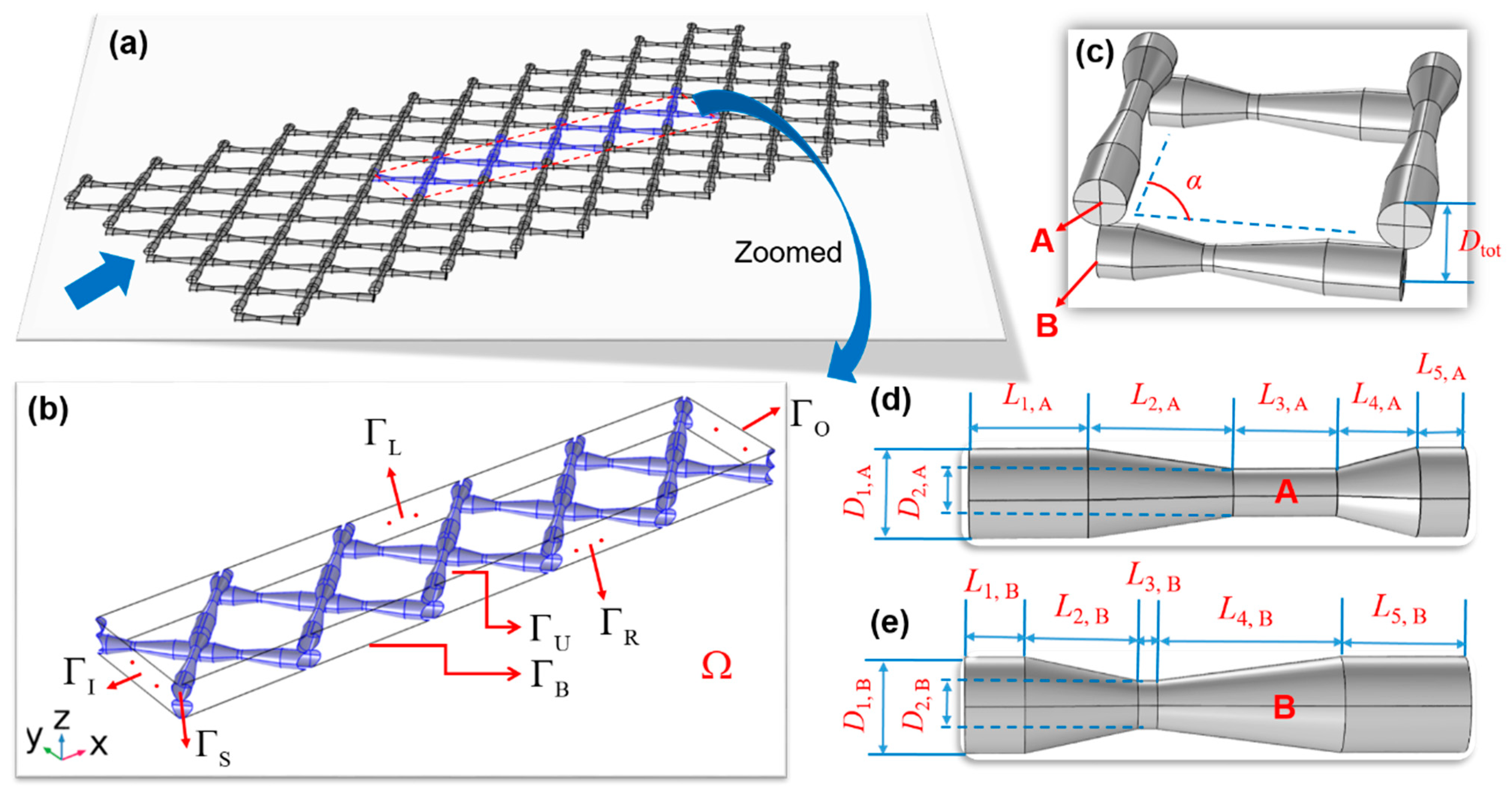
2.1.1. Problem Description

Both the permeable and impermeable wall models in the SWRO desalination consider fluid flow and solute transport, which can be mathematically formulated below [42].

$$\{\begin{array}{ll}\rho (u·\nabla )u=\nabla ·[-PI+\mu (\nabla u+(\nabla u{)}^{\mathrm{T}})],& \mathrm{in}\mathrm{\Omega },\\ \rho \nabla ·u=0,& \mathrm{in}\mathrm{\Omega },\\ D_s{\nabla }^{2}c=u·\nabla c,& \mathrm{in}\mathrm{\Omega },\\ u_{\mathrm{in}}=u_{\mathrm{out}},(\nabla u{)}_{\mathrm{in}}=(\nabla u{)}_{\mathrm{out}},\overline{u}=U,& \mathrm{on}{\mathrm{\Gamma }}_{\mathrm{I}},\\ (\nabla P{)}_{\mathrm{in}}=(\nabla P{)}_{\mathrm{out}},c=c_0,& \mathrm{on}{\mathrm{\Gamma }}_{\mathrm{I}},\\ P=0,-n·D_s\nabla c=0,& \mathrm{on}{\mathrm{\Gamma }}_{\mathrm{O}},\\ J_{\mathrm{W}}=w={\mathcal{G}}_1(L_{\mathrm{P}},P,c),J_{\mathrm{S}}={\mathcal{G}}_2(B,J_{\mathrm{W}},c),& \mathrm{on}{\mathrm{\Gamma }}_{\mathrm{U}}\cup {\mathrm{\Gamma }}_{\mathrm{B}},\\ u_{\mathrm{L}}=u_{\mathrm{R}},P_{\mathrm{L}}=P_{\mathrm{R}},c_{\mathrm{L}}=c_{\mathrm{R}},& \mathrm{on}{\mathrm{\Gamma }}_{\mathrm{L}}\cup {\mathrm{\Gamma }}_{\mathrm{R}},\end{array}$$

(1)

where the governing equations, the Navier–Stokes (N–S) equation, the continuity equation under a laminar flow condition and the convection–diffusion equation are defined in a 3D computational domain ($\mathrm{\Omega }$), or a narrow spacer-filled channel (Figure 2). The variables consist of the velocity vector $u\equiv (u,v,w)$, hydraulic pressure (P) and molar concentration (c). The density ($\rho$) and viscosity ($\mu$) of fluid and the diffusivity ($D_s$) of salt are assumed as constants [42].$L_P$ and $B$ denote water permeability and salt permeability, respectively.

2.1.2. Boundary and Initial Conditions

For the permeable wall model, the permeation flux of water, or water flux ($J_{\mathrm{W}}$), is proportional to the difference ($\mathrm{\Delta }P-\mathrm{\Delta }\pi$) between the transmembrane pressure ($\mathrm{\Delta }P=\mathrm{\Delta }{P}_0-\mathrm{\Delta }{P}_c$) and transmembrane osmotic pressure ($\mathrm{\Delta }\pi$). The specific value is $L_{\mathrm{P}}$. $\mathrm{\Delta }\pi$ is the function of the local concentration on the membrane surfaces. For the impermeable wall model, the permeation flux of water is assumed as zero, and a constant concentration boundary condition is applied on the membrane surfaces. Thus, $J_{\mathrm{W}}$ can be expressed as

$$J_{\mathrm{W}}={\mathcal{G}}_1(L_{\mathrm{P}},P,c)=\{\begin{array}{ll}{L}_{\mathrm{P}}\left[\mathrm{\Delta }{P}_0-\mathrm{\Delta }{P}_c-\mathrm{\Delta }\pi \left(c\right)\right],& for \mathrm{permeable} \mathrm{wall} \mathrm{modeo}\\ 0,& for \mathrm{impermeable} \mathrm{wall} \mathrm{modeo}\end{array}$$

(2)

where $\mathrm{\Delta }{P}_0$ is the inlet transmembrane pressure. The pressure drop ($\mathrm{\Delta }{P}_c$) along the feed direction (x-direction, see Figure 2b) is the difference of the average pressures at the inlet (${\mathrm{\Gamma }}_{\mathrm{I}}$) and outlet (${\mathrm{\Gamma }}_{\mathrm{O}}$), respectively. In the convection–diffusion equation, the boundary conditions for a permeable flux of salt ($J_{\mathrm{S}}$) and a constant concentration ($c_{\mathrm{w},0}$) are enforced on the membrane walls (${\mathrm{\Gamma }}_{\mathrm{U}}\cup {\mathrm{\Gamma }}_{\mathrm{B}}$) for the permeable wall model and impermeable wall model, respectively, as below.

$$\{\begin{array}{ll}{\mathcal{G}}_2(B,J_{\mathrm{W}},c)=n\cdot (-D_{\mathrm{s}}\nabla c+cu)=J_{\mathrm{W}}{c}_{\mathrm{w}}(1-R_{\mathrm{salt}}),& for \mathrm{permeable} \mathrm{wall} \mathrm{model}\\ c_{\mathrm{w}}=c_{\mathrm{w},0}.& for \mathrm{impermeable} \mathrm{wall} \mathrm{model}\end{array}$$

(3)

$c_{\mathrm{w}}$ is the concentration on the membrane walls. The salt rejection ($R_{\mathrm{salt}}$) is defined by

$$R_{\mathrm{salt}}=\frac{J_W}{J_W+B}.$$

(4)

A fully developed boundary condition with an average velocity magnitude and a constant concentration boundary condition ($c=c_0$) are applied at the inlet boundary (${\mathrm{\Gamma }}_{\mathrm{I}}$) for both the permeable and impermeable wall models. The periodic boundary conditions are applied at the lateral boundaries (${\mathrm{\Gamma }}_{\mathrm{L}}\cup {\mathrm{\Gamma }}_{\mathrm{R}}$), which are commonly used in numerical simulation involving structural repeating units (see Figure 2a). For the impermeable wall model, the N–S equation and continuity equation are solved first. The initial velocity and pressure conditions are assumed as constants. The obtained velocity and pressure profiles are used to further calculate the concentration profile by solving the convection– diffusion equation. For the permeable wall model, the calculated velocity, pressure and concentration profiles are solved simultaneously. The simulated results for Case 1 (Commercial SWRO membrane: $L_{\mathrm{P}}$ = 1 L m⁻² h⁻¹ bar⁻¹) are considered as the appropriate initial results to accelerate the solutions for Cases 2–4 (HPMs: $L_{\mathrm{P}}$ = 3 L m⁻² h⁻¹ bar⁻¹; 5 L m⁻² h⁻¹ bar⁻¹; 10 L m⁻² h⁻¹ bar⁻¹).

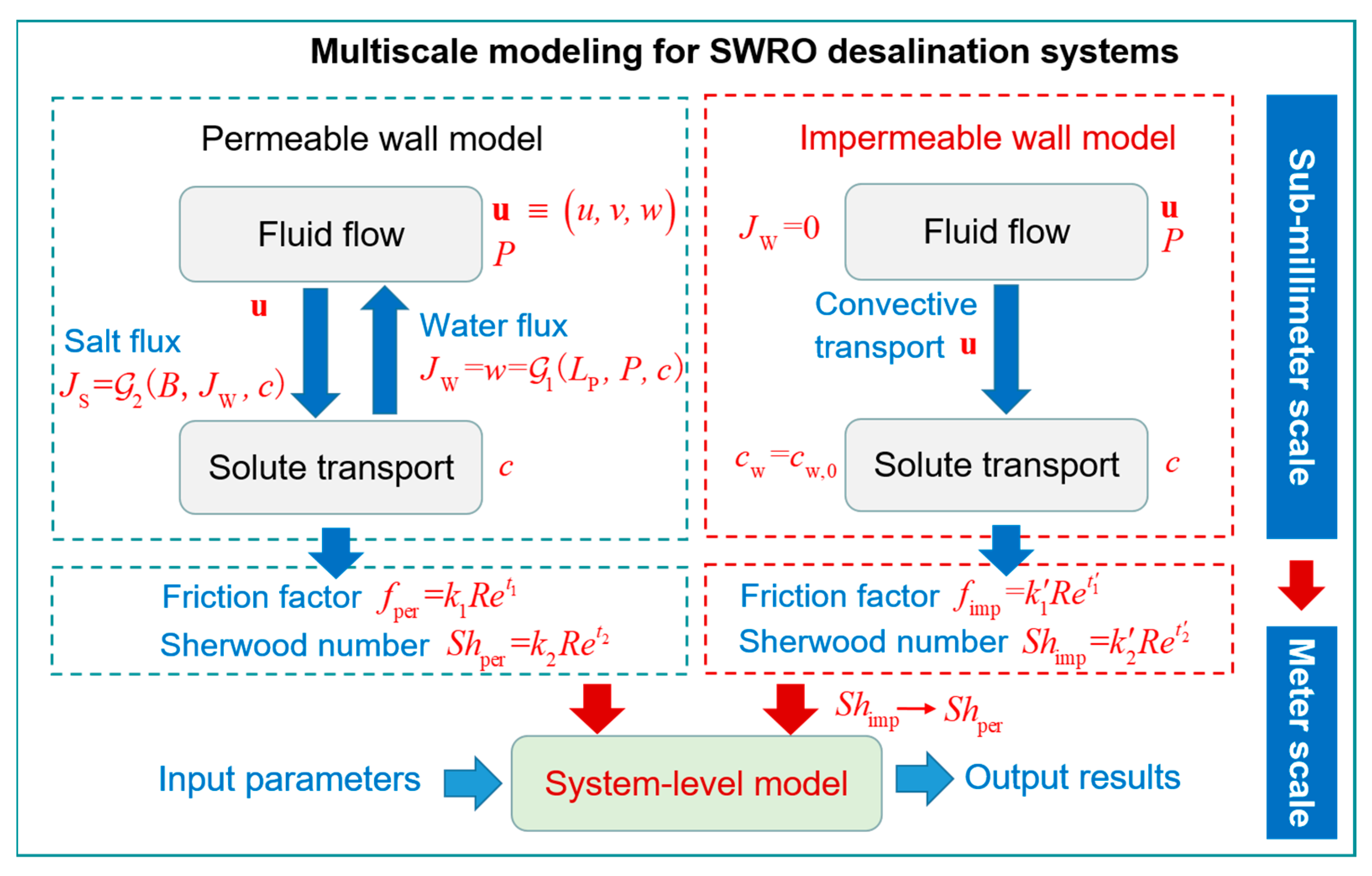
2.2. The Relations Coupling the CFD Model and System-Level Model

After solving Equations (1)–(4), the 3D velocity, pressure and concentration profiles in the spacer-filled channel ($\mathrm{\Omega }$) can be estimated for both the permeable and impermeable wall models. The relations of the friction factor ($f$), Sherwood number ($Sh$) and Reynolds numbers (Re = $\frac{D_H\overline{u}\rho }{\mu }$) are obtained by the fitting curves (f-Re, Sh-Re), namely,

$$\{\begin{array}{ll}{f}_{\mathrm{per}}=k_1{\mathit{Re}}^{t_1},& for \mathrm{permeable} \mathrm{wall} \mathrm{model}\\ S{h}_{\mathrm{per}}=k_2{\mathit{Re}}^{t_2},& for \mathrm{permeable} \mathrm{wall} \mathrm{model}\end{array}$$

(5)

and

$$\{\begin{array}{ll}{f}_{\mathrm{imp}}={k^{\prime }}_1{\mathrm{Re}}^{{t^{\prime }}_1},& for \mathrm{impermeable} \mathrm{wall} \mathrm{model}\\ S{h}_{\mathrm{imp}}={k^{\prime }}_2{\mathrm{Re}}^{{t^{\prime }}_2}.& for \mathrm{impermeable} \mathrm{wall} \mathrm{model}\end{array}$$

(6)

The friction factor ($f_{\mathrm{i}}$) and Sherwood number ($S{h}_{\mathrm{i}}$) are calculated by

$$f_{\mathrm{i}}=-\frac{\mathrm{\Delta }{P}_{c, \mathrm{i}}}{L}{D}_{\mathrm{H}}/\left(\frac{1}{2}{\overline{u}}^2\right), \mathrm{i}=\mathrm{per}, \mathrm{imp}$$

(7)

and

$$S{h}_{\mathrm{i}}=\frac{{\overline{k}}_{\mathrm{m}, \mathrm{i}}{D}_{\mathrm{H}}}{D_{\mathrm{S}}}, \mathrm{i}=\mathrm{per}, \mathrm{imp}$$

(8)

respectively. For a given spacer geometry, the hydraulic diameter ($D_{\mathrm{H}}$) can be identified [29]. Then the pressure drop per unit length along the feed direction (x-direction, see Figure 2b can be calculated by

$$-\frac{\mathrm{\Delta }{P}_{c, \mathrm{i}}}{L}=\frac{\overline{P}(x=0)-\overline{P}(x=L)}{L}, \mathrm{i}=\mathrm{per}, \mathrm{imp}$$

(9)

$\overline{P}(x=L)$ and $\overline{P}(x=0)$ denote the average pressure at the inlet ($x=0$) and outlet ($x=L$). The cell average mass transfer coefficient (${\overline{k}}_{\mathrm{m}, \mathrm{i}}$) is calculated by

$${\overline{k}}_{\mathrm{m}, \mathrm{i}}=\frac{{\displaystyle {\int }_0^L\mathrm{d}x{\displaystyle {\int }_0^W(\frac{-D_{\mathrm{s}}}{c_{\mathrm{r}}-c_{\mathrm{w}}}\cdot \frac{\partial c}{\partial z}{|}_{z=H/2})\mathrm{d}y}}}{{\displaystyle {\int }_0^L\mathrm{d}x{\displaystyle {\int }_0^W\mathrm{d}y}}}, \mathrm{i}=\mathrm{per}, \mathrm{imp}$$

(10)

$L$, $W$ and $H$ denote the length (x-direction), width (y-direction) and height (z-direction) of the computational domain (Figure 2b). It should be pointed out that the estimated Sherwood number using the impermeable wall model (${\overline{k}}_{\mathrm{m}, \mathrm{imp}}$) needs to be corrected using the reported relations [38]

$${\overline{k}}_{\mathrm{m}, \mathrm{per}}={\overline{k}}_{\mathrm{m}, \mathrm{imp}}\left[\psi +{\left(1+0.26{\psi }^{1.4}\right)}^{-1.7}\right], (\psi <20)$$

(11)

$$\psi =\frac{J_W}{{\overline{k}}_{\mathrm{m}, \mathrm{imp}}},$$

(12)

in which $J_W$ is calculated using the system-level model, Equations (13)–(15).

2.3. The System-Level Model for SWRO Desalination at a Meter Scale

Furthermore, we established a system-level model [36,37] that enables us to quantify the effect of spacer geometry on the entire performance of RO desalination.

$$\{\begin{array}{ll}\frac{\mathrm{d}Q}{\mathrm{d}X}=-J_{\mathrm{W}}\cdot A_{\mathrm{tot}}& X=0, Q=Q_0,\\ \frac{\mathrm{d}\left(\mathrm{\Delta }P\right)}{\mathrm{d}X}=-\frac{\rho {\overline{u}}^2}{2D_{\mathrm{H}}}f\cdot \left(n_{\mathrm{mem}}{l}_x\right)& X=0, \mathrm{\Delta }P=\mathrm{\Delta }{P}_0,\\ \frac{\mathrm{d}{w}_{\mathrm{b}}}{\mathrm{d}X}=J_{\mathrm{W}}\cdot \frac{A_{\mathrm{tot}}}{Q}\left(w_{\mathrm{b}}-w_{\mathrm{p}}\right)& X=0, w_{\mathrm{b}}=w_{\mathrm{b},}{}_{ 0},\\ J_{\mathrm{W}}=L_{\mathrm{P}}\left(\mathrm{\Delta }P-\mathrm{\sigma }\cdot \phi R_{\mathrm{salt}}{w}_{\mathrm{w}}\right)& \\ Q=N_{\mathrm{PV}}{n}_{\mathrm{sp}}H{l}_y\epsilon \overline{u},& \end{array}$$

(13)

where $Q$, $\mathrm{\Delta }P$ and $J_{\mathrm{W}}$ are the flow rate, transmembrane pressure and water flux, respectively. $N_{\mathrm{PV}}$, $n_{\mathrm{mem}}$ and $n_{\mathrm{sp}}$ denote the number of pressure vessels, the number of membrane module per pressure vessel and the number of feed spacers per membrane module, respectively. $l_x$ and $l_y$ are the module length parallel to flow and the module length perpendicular to flow, respectively. The porosity, $\epsilon$ is calculated by the formula in previous work [29]. In this paper, the average inlet velocity ($U_0$) is considered as a constant. $w_{\mathrm{b}}$, $w_{\mathrm{p}}$ and $w_{\mathrm{w}}$ denote bulk salinity, permeate salinity and salinity on the membrane walls, respectively. These variables change with respect to various dimensionless length, $X=\frac{x}{n_{\mathrm{mem}}{l}_x}$. The total membrane area, $A_{\mathrm{tot}}$, is calculated by $A_{\mathrm{tot}}= N_{\mathrm{PV}}{n}_{\mathrm{mem}}{A}_0$ ($A_0$: membrane area per membrane module). $\mathrm{\sigma }$ and $\phi$ denote the reflection coefficient and osmotic pressure coefficient, respectively. The salinity on the membrane walls ($w_{\mathrm{w}}$) is calculated by

$$w_{\mathrm{w}}=\frac{w_{\mathrm{p}}}{1-R_{\mathrm{salt}}},$$

(14)

in which $w_{\mathrm{p}}$ can be expressed by

$$w_{\mathrm{p}}=w_{\mathrm{b}}/\left[\exp \left(\ln \frac{J_{\mathrm{W}}}{B}-\frac{J_{\mathrm{W}}}{{\overline{k}}_{\mathrm{m}, \mathrm{per}}}\right)+1\right].$$

(15)

A more detailed derivation for Equation (15) can be found in our latest work [42].

3. Results and Discussion

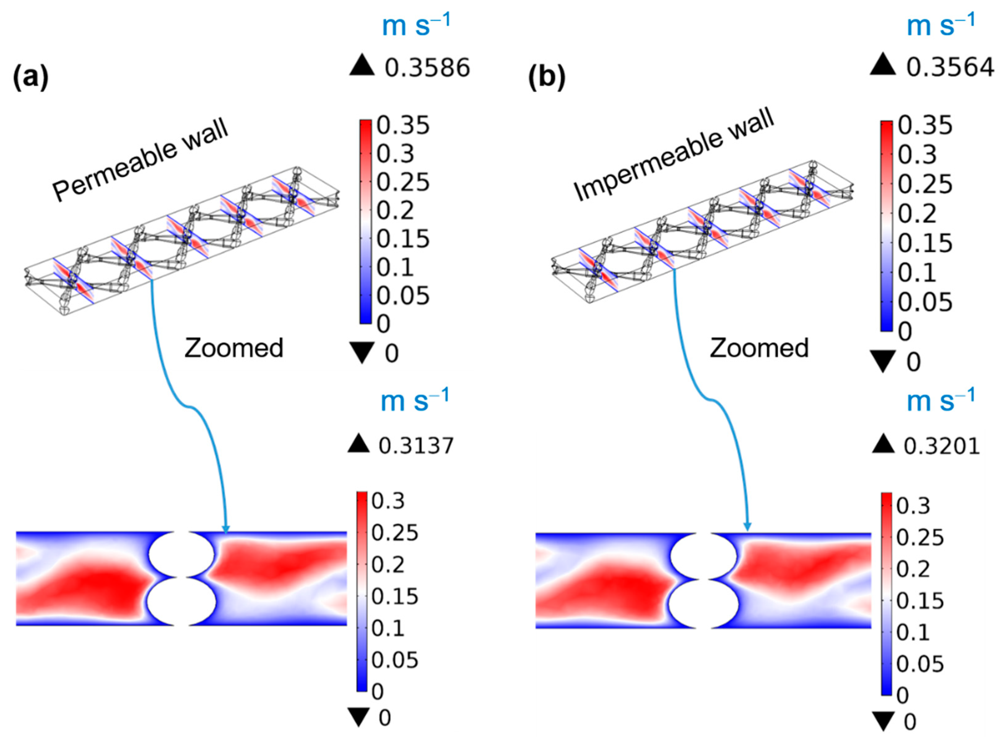
3.1. CFD Simulations

In this paper, the detailed geometry parameters of the feed spacer are listed in

Table 1. The detailed geometrical parameters of the CFD models [44].

Geometrical Parameters		Value
Spacer unit	$L_{1, \mathrm{A}}$ (μm)	234
	$L_{2, \mathrm{A}}$ (μm)	389
	$L_{3, \mathrm{A}}$ (μm)	500
	$L_{4, \mathrm{A}}$ (μm)	696
	$L_{5, \mathrm{A}}$ (μm)	566
	$L_{1, \mathrm{B}}$ (μm)	281
	$L_{2, \mathrm{B}}$ (μm)	535
	$L_{3, \mathrm{B}}$ (μm)	92
	$L_{4, \mathrm{B}}$ (μm)	878
	$L_{5, \mathrm{B}}$ (μm)	599
	$D_{1, \mathrm{A}}$ (μm)	422
	$D_{2, \mathrm{A}}$ (μm)	223
	$D_{1, \mathrm{B}}$ (μm)	445
	$D_{2, \mathrm{B}}$ (μm)	223
	$D_{\mathrm{tot}}$ (μm)	863
	$\alpha$ (°)	90
Computational domain	Length, $L$ (mm)	16.864
	Width, $W$ (mm)	3.3729
	Height, $H$ (mm)	0.853
	Porosity, $\epsilon$ (-)	0.90
	Hydraulic diameter, $D_{\mathrm{H}}$ (mm)	1.058

that are referred to previous literature [44]. The spacer thickness is about 34 mil (863 μm). The number of spatial discrete elements is 1,477,393 (Figure 3), which has comparable precision compared with our previous work [39]. The detailed mesh independence analysis was reported there. Based on the finite element method, Comsol Multiphysics was used to establish and solve the CFD models in this paper. More detailed model parameters can be found in our latest work [42]. The calculated velocity magnitude distributions using the permeable wall model (Figure 4a) and impermeable wall model (Figure 4b) demonstrate that the effect of the permeation flux of water (or water flux) on the cross velocity in the spacer-filled channel is negligible. This is because the water flux (≈10⁻⁵ m/s, see Figure 5a) is much smaller than the cross velocity in the feed channel (Figure 4a), which is consistent with the reported literature [29]. Even for the HPMs systems (e.g., $L_P$ = 5 L m⁻² h⁻¹ bar⁻¹, Figure 5b), this conclusion still holds true. Similarly, the calculated pressure magnitude distribution is basically the same using the permeable wall model (Figure 6a) and impermeable wall model (Figure 6b).

Using the permeable and impermeable wall models, the calculated friction coefficient ($f$) and Sherwood number ($Sh$) are shown in Figure 7a–d and Figure 7e–h, respectively, with the use of a commercial SWRO membrane (Case 1: $L_p$ = 1 L m⁻² h⁻¹ bar⁻¹) and HPMs (Case 2: $L_p$ = 3 L m⁻² h⁻¹ bar⁻¹; Case 3: $L_p$ = 5 L m⁻² h⁻¹ bar⁻¹); Case 4: $L_p$ = 10 L m⁻² h⁻¹ bar⁻¹). It should be noted that the calculated Sherwood number using the impermeable wall model in Figure 7e–h is corrected using Equations (11)–(15). The average errors of the calculated friction coefficient using the impermeable wall model are 0.12%, 0.44%, 0.69% and 1.17%, respectively, for Cases 1–4 compared with that of using the permeable wall model. Correspondingly, the average errors of the estimated Sherwood number are 6.47%, 7.96%, 7.39% and 8.46%, which basically coincide with the reported results in previous work [38]. In an RO system, it is more likely that fouling will occur in the lead elements [45], especially in the condition of high flux. Therefore, we further evaluated the Sherwood number using the impermeable wall model at the system inlet with the errors of 4.25%, 0.27%, 3.49% and 9.51%, respectively. Overall, the accuracy of the impermeable wall model is comparable and acceptable on the prediction of the friction coefficient and Sherwood number versus the permeable wall model. In computational time, the latter one (77.8 h) for each case is about three times than that of the former one (25.3 h). It should be emphasized that the impermeable wall model is only associated with the spacer geometry and inlet velocity, and is independent of other parameters, such as water permeability and operating pressure. Therefore, the Sherwood number with respect to various water permeabilities (Cases 1–4) can be directly calculated using Equations (11)–(15) based on the obtained relations ($f_{\mathrm{imp}}-\mathit{Re}$, $S{h}_{\mathrm{imp}}-\mathit{Re}$). However, the permeable wall model must be recalculated to obtain the Sherwood number when the water permeability or the other conditions change. Thus, the impermeable wall model has a significant advantage in computational efficiency in comparison to the permeable wall model, which can greatly reduce the computational cost, and can be used for the optimal design of the feed spacer.

3.2. Performance Evaluations at a System-Level

Using the system-level model, Equations (13)–(15) coupled with the permeable wall model, Equations (1)–(5), (7)–(10) and the impermeable wall model, Equations (1)–(4), (6)–(12) respectively, the effect of both CFD models on the RO system performance was evaluated. The input parameters for the SWRO system model (Cases 1–4) are listed in

Table 2. The input parameters for SWRO systems in Cases 1–4.

Input Parameters		Value
Operating conditions	Inlet transmembrane pressure, $\mathrm{\Delta }{P}_0$ (bar)	60
	Inlet average velocity magnitude, $U_0$ (m s−1)	0.2
Properties of feed solute	Feed salinity,$w_{\mathrm{b}, 0}$ (ppm)	35,000
	Density, $\rho$ (kg m−3)	1021
	Viscosity, $\mu$ (Pa s)	9.41 × 10−4
	Diffusion coefficient, $D_{\mathrm{s}}$ (m2 s−1)	1.45 × 10−9
	Reflection coefficient, $\mathrm{\sigma }$ (−)	1
	Osmotic pressure coefficient, $\phi$ (bar)	805.1
Membrane properties	Water permeability, $L_{\mathrm{P}}$ (L m−2 h−1 bar−1)	1 (Case1); 3 (Case 2); 5 (Case 3); 10 (Case 4)
	Salt permeability, $B$ (L m−2 h−1)	0.05
Membrane module parameters	Module length parallel to flow, $l_x$ (m)	1
	Module length perpendicular to flow, $l_y$ (m)	1
	Number of feed spacers per element, $n_{\mathrm{sp}}$	23
	Membrane area per membrane module, $A_0$ (m2)	37.2
Module configurations	Number of membrane elements per pressure vessel, $n_{\mathrm{mem}}$	8 (Case1); 5 (Case 2); 3 (Case 3); 2 (Case 4)
	Number of pressure vessels, $N_{\mathrm{pv}}$	30
Efficiencies	Efficiency of high-pressure pump, ${\eta }_{\mathrm{pump}}$ (−)	0.85
	Efficiency of energy recovery device, ${\eta }_{\mathrm{R}}$ (−)	0.95

. The simulated transmembrane pressure ($\mathrm{\Delta }P$), flow rate ($Q$), brine salinity ($w_{\mathrm{b}}$), permeate salinity ($w_{\mathrm{p}}$), permeation flux of water ($J_{\mathrm{W}}$) and $CPF$ along the dimensionless length ($X$) (Inlet: $X$ = 0; Outlet: $X$ = 1) for Cases 1–4 are shown in Figure 8a–f, Figure 9a–f, Figure 10a–f and Figure 11a–f, respectively. Obviously, the simulated results at a system-level based on the impermeable wall model are highly consistent with that of the permeable wall model, even for the HPMs systems. Furthermore, the errors of the calculated average permeate salinity (${\overline{w}}_{\mathrm{p}}$), average permeation flux (${\overline{J}}_{\mathrm{w}}$), maximum CP factor, (max (CPF)), recovery rate ($R_{\mathrm{r}}$), permeate rate ($Q_{\mathrm{p}}$) and $SEC$ are all less than 2% using both the permeable and impermeable wall models. More detailed results are listed in

Table 3. Output results and errors analysis at the system-level coupling with the impermeable wall model (M2) compared with that of using the permeable wall model (M1) with respect to Case 1 ($L_{\mathrm{P}}$ = 1 L m⁻² h⁻¹ bar⁻¹), Case 2 ($L_{\mathrm{P}}$ = 3 L m⁻² h⁻¹ bar⁻¹), Case 3 ($L_{\mathrm{P}}$ = 5 L m⁻² h⁻¹ bar⁻¹) and Case 4 ($L_{\mathrm{P}}$ = 10 L m⁻² h⁻¹ bar⁻¹).

Output Results	Value
	Case 1			Case 2			Case 3			Case 4
	M1	M2	Error	M1	M2	Error	M1	M2	Error	M1	M2	Error
${\overline{w}}_{\mathrm{p}}$ (ppm)	138	139	0.55%	88	89	0.79%	56	56	1.22%	40	40	1.47%
${\overline{J}}_{\mathrm{W}}$ (L m−2 h−1)	18.4	18.3	0.38%	34.1	33.9	0.64%	54.5	54.0	0.99%	81.0	79.9	1.26%
max (CPF) (−)	1.08	1.08	0.32%	1.21	1.21	0.04%	1.32	1.31	0.65%	1.50	1.48	1.86%
$R_{\mathrm{r}}$ (−)	0.43	0.43	0.38%	0.50	0.49	0.64%	0.48	0.47	0.99%	0.47	0.47	1.26%
$Q_{\mathrm{p}}$ (m3 h−1)	164	164	0.38%	190	189	0.64%	182	181	0.99%	181	178	1.26%
$SEC$ (kWh m−3)	2.17	2.17	0.06%	2.11	2.11	0.08%	2.12	2.12	0.12%	2.11	2.12	0.14%

. As the water permeability increases from 1 L m⁻² h⁻¹ bar⁻¹ to 10 L m⁻² h⁻¹ bar⁻¹, the maximum CP factor at the system inlet can reach up to about 1.50, which will intensify the membrane fouling. Therefore, it is crucial to enhance the mass transfer with a pressure loss penalty when the SWRO system is operated at higher flux. To achieve this, the spacer design and improvement of the cross velocity or unsteady-state shear technologies [46] are alternative methods.

4. Conclusions and Outlook

In this paper, we propose a multiscale model framework that couples the CFD models with a permeable wall and an impermeable wall, respectively, and the SWRO model at the system level. The simulated results indicate that the CFD simulations (e.g., velocity, pressure) and the system simulations (e.g., SEC, average permeation flux) using the permeable and impermeable wall models are basic unanimous (error < 2%). The error of the estimated Sherwood number at the system inlet using both models is smaller than 10%, even under extremely high-flux conditions (≈200 L m⁻² h⁻¹ at system inlet). Furthermore, the impermeable wall model is one-way coupled, which can greatly reduce the computational time compared to the fully coupled permeable wall model. The proposed multiscale framework coupling the impermeable wall model enables the feed spacer design and system design simultaneously for high permeability RO/NF membrane systems. Nevertheless, the impermeable wall model still has some limitations. On the one hand, it cannot accurately predict the local CP due to the assumed constant concentration boundary condition on membrane walls. On the other hand, the correct relations from ${\overline{k}}_{\mathrm{m}, \mathrm{imp}}$ to ${\overline{k}}_{\mathrm{m}, \mathrm{per}}$ must satisfy the condition of $J_{\mathrm{W}}/{\overline{k}}_{\mathrm{m}, \mathrm{imp}}<20$.

References

1. Anis, S.; Hashaikeh, R.; Hilal, N. Microfiltration membrane processes: A review of research trends over the past decade. J. Water Process. Eng. 2019, 32, 100941. [Google Scholar] [CrossRef]
2. Mouiya, M.; Abourriche, A.; Bouazizi, A.; Benhammou, A.; El Hafiane, Y.; Abouliatim, Y.; Nibou, L.; Oumam, M.; Ouammou, M.; Smith, A.; et al. Flat ceramic microfiltration membrane based on natural clay and Moroccan phosphate for desalination and industrial wastewater treatment. Desalination 2018, 427, 42–50. [Google Scholar] [CrossRef]
3. Al Aani, S.; Mustafa, T.; Hilal, N. Ultrafiltration membranes for wastewater and water process engineering: A comprehensive statistical review over the past decade. J. Water Process. Eng. 2020, 35, 101241. [Google Scholar] [CrossRef]
4. Brover, S.; Lester, Y.; Brenner, A.; Sahar-Hadar, E. Optimization of ultrafiltration as pre-treatment for seawater RO desalination. Desalination 2022, 524, 115478. [Google Scholar] [CrossRef]
5. Zhou, D.; Zhu, L.; Fu, Y.; Zhu, M.; Xue, L. Development of lower cost seawater desalination processes using nanofiltration technologies—A review. Desalination 2015, 376, 109–116. [Google Scholar] [CrossRef]
6. Wafi, M.; Hussain, N.; Abdalla, O.E.-S.; Al-Far, M.; Al-Hajaj, N.; Alzonnikah, K. Nanofiltration as a cost-saving desalination process. SN Appl. Sci. 2019, 1, 751. [Google Scholar] [CrossRef] [Green Version]
7. Qasim, M.; Badrelzaman, M.; Darwish, N.; Darwish, N.; Hilal, N. Reverse osmosis desalination: A state-of-the-art review. Desalination 2019, 459, 59–104. [Google Scholar] [CrossRef] [Green Version]
8. Lim, Y.; Goh, K.; Kurihara, M.; Wang, R. Seawater desalination by reverse osmosis: Current development and future challenges in membrane fabrication—A review. J. Membr. Sci. 2021, 629, 119292. [Google Scholar] [CrossRef]
9. Galama, A.; Saakes, M.; Bruning, H.; Rijnaarts, H.; Post, J. Seawater predesalination with electrodialysis. Desalination 2014, 342, 61–69. [Google Scholar] [CrossRef]
10. Al-Amshawee, S.; Yunus, M.; Azoddein, A.; Hassell, D.; Dakhil, I.; Hasan, H. Electrodialysis desalination for water and wastewater: A review. Chem. Eng. J. 2020, 380, 122231. [Google Scholar] [CrossRef]
11. Yadav, A.; Labhasetwar, P.; Shahi, V. Membrane distillation using low-grade energy for desalination: A review. J. Environ. Chem. Eng. 2021, 9, 105818. [Google Scholar] [CrossRef]
12. Yadav, A.; Patel, R.; Singh, C.; Labhasetwar, P.; Shahi, V. Experimental study and numerical optimization for removal of methyl orange using polytetrafluoroethylene membranes in vacuum membrane distillation process. Colloids Surf. A Physicochem. Eng. Asp. 2022, 635, 128070. [Google Scholar] [CrossRef]
13. Feinberg, B.; Ramon, G.; Hoek, E. Thermodynamic analysis of osmotic energy recovery at a reverse osmosis desalination plant. Environ. Sci. Technol. 2013, 47, 2982–2989. [Google Scholar] [CrossRef] [PubMed]
14. Lim, Y.; Ma, Y.; Chew, J.; Wang, R. Assessing the potential of highly permeable reverse osmosis membranes for desalination: Specific energy and footprint analysis. Desalination 2022, 533, 115771. [Google Scholar] [CrossRef]
15. Zhang, Z.; Wu, Y.; Luo, L.; Li, G.; Li, Y.; Hu, H. Application of disk tube reverse osmosis in wastewater treatment: A review. Sci. Total Environ. 2021, 792, 148291. [Google Scholar] [CrossRef] [PubMed]
16. Colla, V.; Branca, T.; Rosito, F.; Lucca, C.; Vivas, B.; Delmiro, V. Sustainable Reverse Osmosis application for wastewater treatment in the steel industry. J. Clean. Prod. 2016, 130, 103–115. [Google Scholar] [CrossRef]
17. Licona, K.; Geaquinto, L.; Nicolini, J.; Figueiredo, N.; Chiapetta, S.; Habert, A.; Yokoyama, L. Assessing potential of nanofiltration and reverse osmosis for removal of toxic pharmaceuticals from water. J. Water Process. Eng. 2018, 25, 195–204. [Google Scholar] [CrossRef]
18. Lin, Y.; Chiou, J.; Lee, C. Effect of silica fouling on the removal of pharmaceuticals and personal care products by nanofiltration and reverse osmosis membranes. J. Hazard. Mater. 2014, 277, 102–109. [Google Scholar] [CrossRef]
19. Bejaoui, I.; Mnif, A.; Hamrouni, B. Performance of Reverse Osmosis and Nanofiltration in the Removal of Fluoride from Model Water and Metal Packaging Industrial Effluent. Sep. Sci. Technol. 2014, 49, 1135–1145. [Google Scholar] [CrossRef]
20. Ndiaye, P.; Moulin, P.; Dominguez, L.; Millet, J.; Charbit, F. Removal of fluoride from electronic industrial effluent by RO membrane separation. Desalination 2005, 173, 25–32. [Google Scholar] [CrossRef]
21. Zhao, D.; Japip, S.; Zhang, Y.; Weber, M.; Maletzko, C.; Chung, T. Emerging thin-film nanocomposite (TFN) membranes for reverse osmosis: A review. Water Res. 2020, 173, 115557. [Google Scholar] [CrossRef]
22. Rahmawati, R.; Bilad, M.; Nawi, N.; Wibisono, Y.; Suhaimi, H.; Shamsuddin, N.; Arahman, N. Engineered spacers for fouling mitigation in pressure driven membrane processes: Progress and projection. J. Environ. Chem. Eng. 2021, 9, 106285. [Google Scholar] [CrossRef]
23. Lin, W.; Zhang, Y.; Li, D.; Wang, X.; Huang, X. Roles and performance enhancement of feed spacer in spiral wound membrane modules for water treatment: A 20-year review on research evolvement. Water Res. 2021, 198, 117146. [Google Scholar] [CrossRef]
24. Fimbres-Weihs, G.; Wiley, D. Review of 3D CFD modeling of flow and mass transfer in narrow spacer-filled channels in membrane modules. Chem. Eng. Process. 2010, 49, 759–781. [Google Scholar] [CrossRef]
25. Anqi, A.; Alkhamis, N.; Oztekin, A. Computational study of desalination by reverse osmosis—Three-dimensional analyses. Desalination 2016, 388, 38–49. [Google Scholar] [CrossRef]
26. Lin, W.; Shao, R.; Wang, X.; Huang, X. Impacts of non-uniform filament feed spacers characteristics on the hydraulic and anti-fouling performances in the spacer-filled membrane channels: Experiment and numerical simulation. Water Res. 2020, 185, 116251. [Google Scholar] [CrossRef] [PubMed]
27. Foo, K.; Liang, Y.; Weihs, G. CFD study of the effect of SWM feed spacer geometry on mass transfer enhancement driven by forced transient slip velocity. J. Membr. Sci. 2020, 597, 117643. [Google Scholar] [CrossRef]
28. Singh, C.; Yadav, A.; Kumar, A. Numerical simulations of the effect of spacer filament geometry and orientation on the performance of the reverse osmosis process. Colloid. Surface A 2022, 650, 129664. [Google Scholar] [CrossRef]
29. Li, M.; Bui, T.; Chao, S. Three-dimensional CFD analysis of hydrodynamics and concentration polarization in an industrial RO feed channel. Desalination 2016, 397, 194–204. [Google Scholar] [CrossRef]
30. Lin, W.; Lei, J.; Wang, Q.; Wang, X.-m.; Huang, X. Performance enhancement of spiral-wound reverse osmosis membrane elements with novel diagonal-flow feed channels. Desalination 2022, 523, 115447. [Google Scholar] [CrossRef]
31. Yadav, A.; Singh, C.; Patel, R.; Kumar, A.; Labhasetwar, P. Investigations on the effect of spacer in direct contact and air gap membrane distillation using computational fluid dynamics. Colloids Surf. A Physicochem. Eng. Asp. 2022, 654, 130111. [Google Scholar] [CrossRef]
32. Koutsou, C.; Yiantsios, S.; Karabelas, A. A numerical and experimental study of mass transfer in spacer-filled channels: Effects of spacer geometrical characteristics and Schmidt number. J. Membr. Sci. 2009, 326, 234–251. [Google Scholar] [CrossRef]
33. Completo, C.; Semiao, V.; Geraldes, V. Efficient CFD-based method for designing cross-flow nanofiltration small devices. J. Membr. Sci. 2016, 500, 190–202. [Google Scholar] [CrossRef]
34. Fimbres-Weihs, G.; Wiley, D. Numerical study of mass transfer in three-dimensional spacer-filled narrow channels with steady flow. J. Membr. Sci. 2007, 306, 228–243. [Google Scholar] [CrossRef]
35. Shakaib, M.; Hasani, S.; Mahmood, M. CFD modeling for flow and mass transfer in spacer-obstructed membrane feed channels. J. Membr. Sci. 2009, 326, 270–284. [Google Scholar] [CrossRef]
36. Liang, Y.; Toh, K.; Weihs, G.F. 3D CFD study of the effect of multi-layer spacers on membrane performance under steady flow. J. Membr. Sci. 2019, 580, 256–267. [Google Scholar] [CrossRef]
37. Toh, K.; Liang, Y.; Lau, W.; Weihs, G. The techno-economic case for coupling advanced spacers to high-permeance RO membranes for desalination. Desalination 2020, 491, 114534. [Google Scholar] [CrossRef]
38. Geraldes, V.; Afonso, M. Generalized mass-transfer correction factor for nanofiltration and reverse osmosis. AIChE J. 2006, 52, 3353–3362. [Google Scholar] [CrossRef]
39. Luo, J.; Li, M.; Heng, Y. A hybrid modeling approach for optimal design of non-woven membrane channels in brackish water reverse osmosis process with high-throughput computation. Desalination 2020, 489, 114463. [Google Scholar] [CrossRef]
40. Chen, Q.; Luo, J.; Heng, Y. High-Throughput Optimal Design of Spacers Using Triply Periodic Minimal Surfaces in BWRO. Separations 2022, 9, 62. [Google Scholar] [CrossRef]
41. Gu, J.; Luo, J.; Li, M.; Huang, C.; Heng, Y. Modeling of pressure drop in reverse osmosis feed channels using multilayer artificial neural networks. Chem. Eng. Res. Des. 2020, 159, 146–156. [Google Scholar] [CrossRef]
42. Luo, J.; Li, M.; Hoek, E.; Heng, Y. Supercomputing and machine learning-aided optimal design of high permeability seawater reverse osmosis membrane systems. Sci. Bull. 2023, in press. [Google Scholar] [CrossRef] [PubMed]
43. Li, F.; Meindersma, W.; Haan, A.; Reith, T. Optimization of commercial net spacers in spiral wound membrane modules. J. Membr. Sci. 2002, 208, 289–302. [Google Scholar] [CrossRef] [Green Version]
44. Bucs, S.; Radu, A.; Lavric, V.; Vrouwenvelder, J.; Picioreanu, C. Effect of different commercial feed spacers on biofouling of reverse osmosis membrane systems: A numerical study. Desalination 2014, 343, 26–37. [Google Scholar] [CrossRef]
45. Al-Amoudi, A.; Lovitt, R. Fouling strategies and the cleaning system of NF membranes and factors affecting cleaning efficiency. J. Membr. Sci. 2007, 303, 4–28. [Google Scholar] [CrossRef]
46. Zamani, F.; Chew, J.; Akhondi, E.; Krantz, W.; Fane, A. Unsteady-state shear strategies to enhance mass-transfer for the implementation of ultrapermeable membranes in reverse osmosis: A review. Desalination 2015, 356, 328–348. [Google Scholar] [CrossRef]
Figure 1. The multiscale modeling framework for SWRO desalination that integrates the permeable wall model and the impermeable wall model.
Separations 10 00134 g001
Figure 2. (a) Spacer sheet; (b) The computational domain (spacer-filled channel); (c) A spacer unit; (d) Filament A; and (e) Filament B.
Separations 10 00134 g002
Figure 3. The geometric model discretization for (a) the computational domain and (b) the zoomed spacer section.
Separations 10 00134 g003
Figure 4. The velocity magnitude distributions with an inlet average velocity magnitude of 0.15 m s−1 using (a) the permeable wall model (Case 1: L P = 1 L m−2 h−1 bar−1) and (b) the impermeable wall model.
Separations 10 00134 g004
Figure 5. The water flux with inlet average velocity magnitude of 0.15 m s−1 using the permeable wall model for (a) the commercial membrane ( L P = 1 L m−2 h−1 bar−1) and (b) the HPM ( L P = 5 L m−2 h−1 bar−1) systems.
Separations 10 00134 g005
Figure 6. The pressure magnitude distributions with an inlet average velocity magnitude of 0.15 m s−1 using (a) the permeable wall model and (b) the impermeable wall model.
Separations 10 00134 g006
Figure 7. The friction coefficient ( f ) and and Sherwood number ( Sh ) with respect to various Reynolds numbers (Re) using the impermeable wall model and the permeable wall model for Case 1 (a,e) ( L P = 1 L m−2 h−1 bar−1), (b,f) Case 2 ( L P = 3 L m−2 h−1 bar−1), (c,g) Case 3 ( L P = 5 L m−2 h−1 bar−1) and (d,h) Case 4 ( L P = 10 L m−2 h−1 bar−1).
Separations 10 00134 g007
Figure 8. The simulated results at the system level using the impermeable and permeable wall models with the feed salinity ( w ¯ b ,   0 = 35,000 ppm), water recovery ( R r ,   0 = 50%), pump efficiency (0.85), energy recovery device efficiency (0.95) and water permeability ( L p = 1 L m−2 h−1 bar−1). (a) Transmembrane pressure, Δ P (bar), (b) Flow rate, Q (m3 h−1), (c) Brine salinity, w b (ppm), (d) Permeate salinity, w p (ppm), (e) Permeation flux of water, J W (L m−2 h−1), (f) CP factor, C P F (−) along the dimensionless length ( X ).
Separations 10 00134 g008
Figure 9. The simulated results at the system level using the impermeable and permeable wall models with the feed salinity ( w ¯ b ,   0 = 35,000 ppm), water recovery ( R r ,   0 = 50%), pump efficiency (0.85), energy recovery device efficiency (0.95) and water permeability ( L p = 3 L m−2 h−1 bar−1). (a) Transmembrane pressure, Δ P (bar), (b) Flow rate, Q (m3 h−1), (c) Brine salinity, w b (ppm), (d) Permeate salinity, w p (ppm), (e) Permeation flux of water, J W (L m−2 h−1), (f) CP factor, C P F (−) along the dimensionless length ( X ).
Separations 10 00134 g009
Figure 10. The simulated results at the system level using the impermeable and permeable wall models with the feed salinity ( w ¯ b ,   0 = 35,000 ppm), water recovery ( R r ,   0 = 50%), pump efficiency (0.85), energy recovery device efficiency (0.95) and water permeability ( L p = 5 L m−2 h−1 bar−1). (a) Transmembrane pressure, Δ P (bar), (b) Flow rate, Q (m3 h−1), (c) Brine salinity, w b (ppm), (d) Permeate salinity, w p (ppm), (e) Permeation flux of water, J W (L m−2 h−1), (f) CP factor, C P F (−) along the dimensionless length ( X ).
Separations 10 00134 g010
Figure 11. The simulated results at the system level using the impermeable and permeable wall models with the feed salinity ( w ¯ b ,   0 = 35,000 ppm), water recovery ( R r ,   0 = 50%), pump efficiency (0.85), energy recovery device efficiency (0.95) and water permeability ( L p = 10 L m−2 h−1 bar−1). (a) Transmembrane pressure, Δ P (bar), (b) Flow rate, Q ( m3 h−1), (c) Brine salinity, w b (ppm), (d) Permeate salinity, w p (ppm), (e) Permeation flux of water, J W (L m−2 h−1), (f) CP factor, C P F (−) along the dimensionless length ( X ).
Separations 10 00134 g011