Article

An Electricity Consumption Disaggregation Method for HVAC Terminal Units in Sub-Metered Buildings Based on CART Algorithm

1
Beijing Key Laboratory of Green Built Environment and Energy Efficient Technology, Beijing University of Technology, Beijing 100124, China
2
College of Architecture and Urban Planning, Tongji University, Shanghai 201804, China
*
Author to whom correspondence should be addressed.
Buildings 2023, 13(4), 967; https://doi.org/10.3390/buildings13040967
Submission received: 9 March 2023 / Revised: 27 March 2023 / Accepted: 28 March 2023 / Published: 6 April 2023
(This article belongs to the Special Issue Study on Building Energy Efficiency Related to Simulation Models)

Abstract

:
Obtaining reliable and detailed energy consumption information about building service (BS) systems is an essential prerequisite for identifying energy-saving potential and improving energy efficiency of a building. Therefore, in recent years, energy sub-metering systems have been widely implemented in public buildings in China. A majority of electrical systems and equipment can be directly metered. However, in actual sub-metering systems, the terminal units of heating, ventilation and air conditioning (HVAC) systems, such as fan coils, air handling units and so on, are often mixed with the lighting-plug circuit. This mismatch between theoretical sub-metering systems and actual electricity supply circuits constitutes a lot of challenges in BS system management and control optimization. This study proposed an indirect method to disaggregate the energy consumption of HVAC terminal units from mixed sub-metering data based on the CART algorithm. This method was demonstrated in two buildings in Shanghai. The case study results show that the weighted mean absolute percentage errors (WMAPE) are within 5% and 15% during working hours in the cooling and heating seasons, respectively.

1. Introduction

Buildings are one of the world’s largest energy consumers and carbon emission producers. According to the tracking report from the International Energy Agency (IEA), the operation of buildings accounted for about 30% of global final energy consumption and 27% of total energy system emission in 2021. About 19% of energy-related carbon emission came from the generation of electricity and heat used in buildings. Compared to 2010, electricity consumption increased by 30% in 2021 [1]. With the widespread use of central heating, ventilation and air conditioning (HVAC) systems, the energy consumption per unit area of public buildings in China increased from 17 kgce/m2 in 2001 to more than 24.7 kgce/m2 in 2020 [2]. Various energy conservation measures need to be adopted to improve building energy efficiency and reduce carbon emission, which increases the possibility of achieving carbon neutrality in China by 2060.
At the building operation stage, accurate building system operation data are indispensable for optimizing HVAC system control strategy and analyzing building energy-saving potential. Therefore, it is very important to obtain accurate building energy consumption data, especially data of HVAC units.

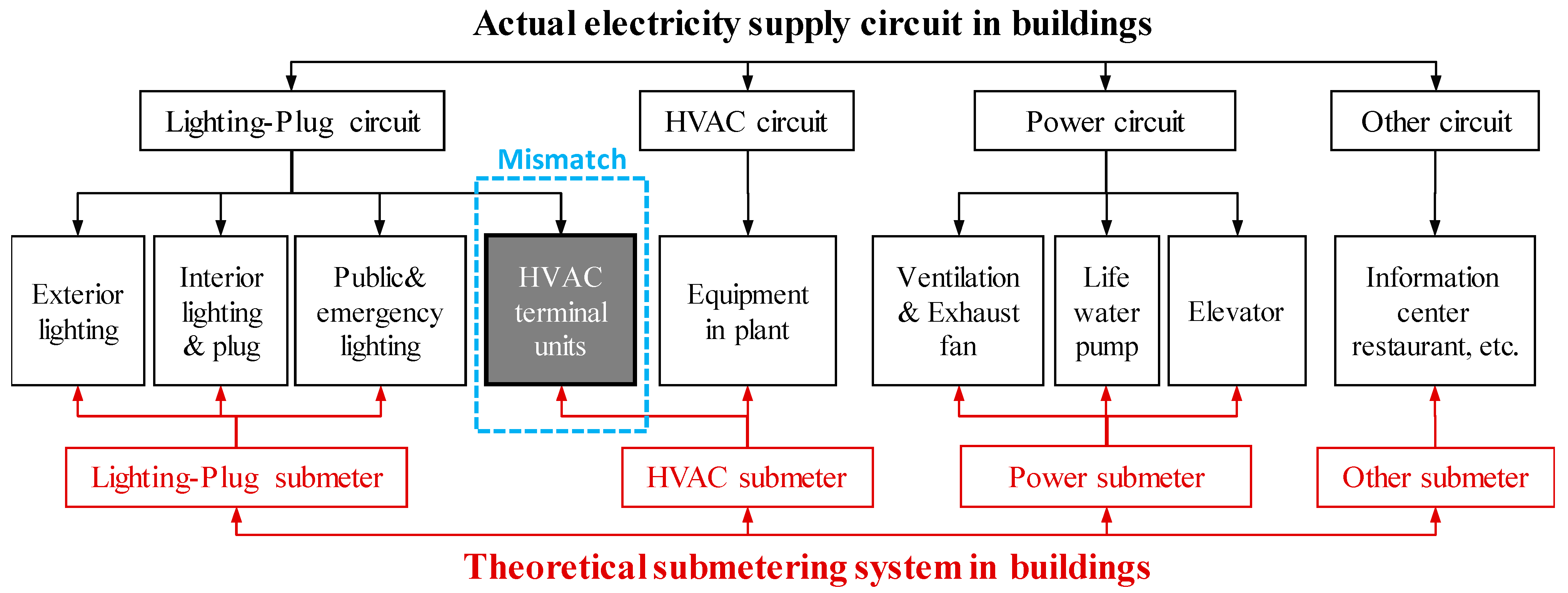
1.1. The Status Quo of Sub-Metering Systems

In recent years, energy sub-metering systems have been widely implemented in various buildings. A majority of electrical systems and equipment can be directly monitored and metered. Electricity sub-metering was first proposed by Dr. Hart in 1992 [3]. In 2008, the California Public Utilities Commission (CPUC) adopted a resolution to carry out electricity sub-metering in multi-story commercial buildings [4]. In 2007, the Chinese government issued document No. 558, declaring that a special compensation would be used for building energy monitoring platforms [5]. Large-scale investigations on public building energy consumption have been conducted in Shanghai since 1995 and have then extended to other cities in China, including Beijing, Tianjin, Changsha and Wuhan [6,7,8]. Statistical data from Shanghai show that more than 1400 large public buildings (the total area exceeding 60 million m2) have installed a sub-metering system [9].
The technical guidelines for electricity sub-metering data collection in China’s document No. 114 clearly stipulate that an entire building’s electricity consumption should be recorded by four primary sub-metering circuits, including the lighting-plug circuit, HVAC circuit, power circuit and other circuit [10]. This electricity sub-metering classification diagram is illustrated in Figure 1. The technical guidelines also point out that the electricity consumption of HVAC terminal units (e.g., fan coils and variable air volume (VAV) boxes) can be recorded in the lighting-plug circuit because, based on existing electricity-supply circuit design, HVAC terminals are usually plugged in the lighting-plug circuit [10]. Therefore, there is a grey area between an actual sub-metering model (black lines) and the theoretical (red lines) sub-metering classification model (shown in Figure 1). Additionally, the HVAC electricity consumption obtained from a building sub-metering system would be lower than the actual HVAC electricity consumption. In China, this is a common phenomenon. We conducted a survey of about 1400 buildings with a sub-metering system in Shanghai and found that only two buildings had direct sub-meters of HVAC terminal units. In most buildings, it is still impossible to obtain the electricity consumption of HVAC terminal units directly.
However, accurate sub-metering data are extremely significant in many fields, including evaluating the energy-saving potential of buildings [11], selecting suitable energy efficiency technology [12], reducing carbon emissions of building operation [13], and securing the optimal control of HVAC systems [14]. Therefore, it is necessary to establish an indirect method to acquire the electricity consumption of HVAC terminal units.

1.2. Non-Intrusive Load Monitoring (NILM) Method

In the early 1990s, researchers introduced a method called non-intrusive load monitoring (NILM) to measure the electricity consumption of facilities in buildings [15,16,17,18]. This method can also be used to distinguish equipment’s on/off signals (e.g., current, voltage, active power and reactive power) and record the power and operational duration. This method is eminently suitable for residential buildings with low-power appliances and simple electricity supply systems [19,20]. Norford et al. applied a NILM method to small-scale commercial buildings [21]. They proposed a load disaggregation model to distinguish the load of air-conditioning systems from other electrical appliances with similar power levels or operation time [22].
NILM methods can be divided into four categories: machine learning method, sparse coding, dynamic time warping (DTW) and Fourier analysis. Machine learning is one of the most popular approaches because it is easy to use and has high accuracy. Rafsanjani et al. combined Density-based Spatial Clustering of Applications with Noise (DBSCAN) algorithm and quadratic discriminant analysis (QDA) to disaggregate total building energy loads into individual energy consumption [23,24]. Kaselimi et al. proposed a Bayesian-optimized Bidirectional LSTM regression model to disaggregate the energy consumption of residential buildings [25]. Schirmer et al. used feed-forward Deep Neural Networks (DNNs), k-Nearest Neighbors (KNNs), Random Forests (RFs) and Support Vector Machines (SVMs) to disaggregate the electricity consumption of residential buildings separately [26]. Kaselimi M et al. proposed a Convolutional Neural Network (CNN)-based structure to estimate the current state of appliances in residential buildings [27]. Yang D et al. proposed an event-driven NILM method based on CNN to extract the energy consumption behavior of occupants [28]. Faustine A et al. proposed a UNet-NILM method based on multi-label learning strategy and multi-target quantile regression to detect the state and power of electrical appliances [29]. Xia et al. presented a deep Long Short-Term Memory (LSTM) model for load disaggregation. In this model, an encoder–decoder structure was designed to solve the problem of time dependency in multi-state devices [30]. Guo et al. presented a load disaggregation method based on combinatorial optimization to disaggregate the electricity load of residential buildings [31]. Monteiro et al. disaggregated residential buildings’ electricity load by using Multi-layer Perceptron (MLP), LSTM and Convolutional Neural Network (CNN) [32]. Samadi and Fattahi used K-means method to cluster the daily load profiles of buildings and calculated the common load and occupancy load in different day types [33]. Xiao et al. applied RF for the cooling load disaggregation of office buildings [34]. Athanasiadis C et al. proposed a real-time NILM method, including an event detection algorithm, a CNN classifier and a power estimation algorithm, to estimate the energy consumption of household appliances [35]. Shao et al. proposed a load disaggregation approach based on temporal motif mining. This approach used a clustering method to detect the power of household devices [36]. Burak Gunay et al. proposed an electricity end-use disaggregation method based on regression models for commercial buildings [37]. Zaeri et al. applied multiple linear regression models to disaggregate the electricity and heating consumption in commercial buildings. These models were estimated by a least-square solver with a genetic algorithm [38].
Sparse coding and DTW algorithm are widely used in NILM methods. Elafoudi et al. proposed a NILM method based on DTW algorithm to disaggregate the electricity consumption of residential building devices [39]. Kolter et al. used a sparse coding algorithm to train models for each device in a residential building with electricity consumption and applied these models to predict the electricity consumption of each device [40]. Matsui et al. applied a 0–1 sparse coding method to disaggregate the energy consumption of electric appliances from the total energy consumption of residential buildings [41].
Fourier analysis can be used to disaggregate different loads in the frequency domain. Dhar et al. took advantage of a Fourier series model to simulate real-time energy consumption of some campus buildings in Texas and obtained satisfactory results [42,43,44]. Ji et al. applied Fourier series models to disaggregate hourly electricity consumption of HVAC system terminal units from mixed lighting-plug sub-meters of commercial buildings [45]. The accuracy of the calculation results is high, although, in this study, the division of the date type is slightly rough, and a standardized and programmed calculation process is not achieved. Table 1 summarizes the details of above studies.
Comprehensive information and detailed monitoring data of HVAC systems are the basis for building energy analysis and system control [46]. However, most previous studies have disaggregated the total electricity consumption of residential buildings into individual devices or the total electricity consumption of public buildings into system levels only. It is difficult for most existing commercial buildings to obtain the electricity consumption of HVAC terminal units directly. Therefore, an effective method is still needed to disaggregate the electricity consumption of HVAC terminal units from mixed sub-metering data.
Previous studies on the characteristics of building electricity consumption have provided a theoretical basis for the disaggregation of mixed sub-metering data. The research conducted by Pandit et al. indicated that the electricity consumption of most commercial buildings follows an obviously periodical pattern [47]. The research by Braun et al. showed that sinusoidal functions could simulate the electricity demand in buildings [48]. They used a trigonometric formula to simulate the electricity consumption of commercial buildings. Afterward, the research by Claridge et al. indicated that the electricity consumption of lights and office equipment varied periodically and was not sensitive to outdoor weather conditions [49]. The investigations by Dhar et al. showed that for commercial buildings, electricity consumption had clear differences between weekdays and non-workdays [42,43,44]. Additionally, electricity consumption in different meteorological conditions should be treated differently. In our own previous research work, we used EnergyPlus to simulate the energy consumption of HVAC terminal units of a whole building. However, this method is time consuming because a detailed architectural model needs to be established and calibrated. When applied in another building, the model needs to be rebuilt [50].
It is a common practical problem that the electricity consumption of HVAC terminal units is mixed with lighting-plug sub-metering systems in most public buildings in China. This is one of the reasons why sub-metering data quality is poor in China. Many previous research studies focused on electricity consumption disaggregation for residential buildings, while only few research studies discussed the problem for public buildings. Some existing research studies adopted a Fourier series model in sub-metering data disaggregation. However, this algorithm is not suitable for categorical data. Different building types may require different date-type categorization methods. Therefore, in this study, we adopted a CART algorithm to disaggregate the real-time electricity consumption of the terminal units in a HVAC system, and we proposed a general calculation process to make it easier for other users, which would improve the data quality of sub-metering data in building energy management. The main novelties of this study are listed as follows:
(1)
This study adopts a CART algorithm to disaggregate the real-time electricity consumption of HVAC terminal units. It makes up for the deficiency that the Fourier series model is not suitable for categorical data.
(2)
A general disaggregation framework is proposed. It can be easily extended to different cases without constructing physical building energy models.
In this article, the methodology and model establishment processes are described in Section 2. In Section 3, two case studies in Shanghai are used to illustrate how to apply the proposed method. Discussions and limitations are presented in Section 4, and the conclusions are outlined in Section 5.

2. Methodology

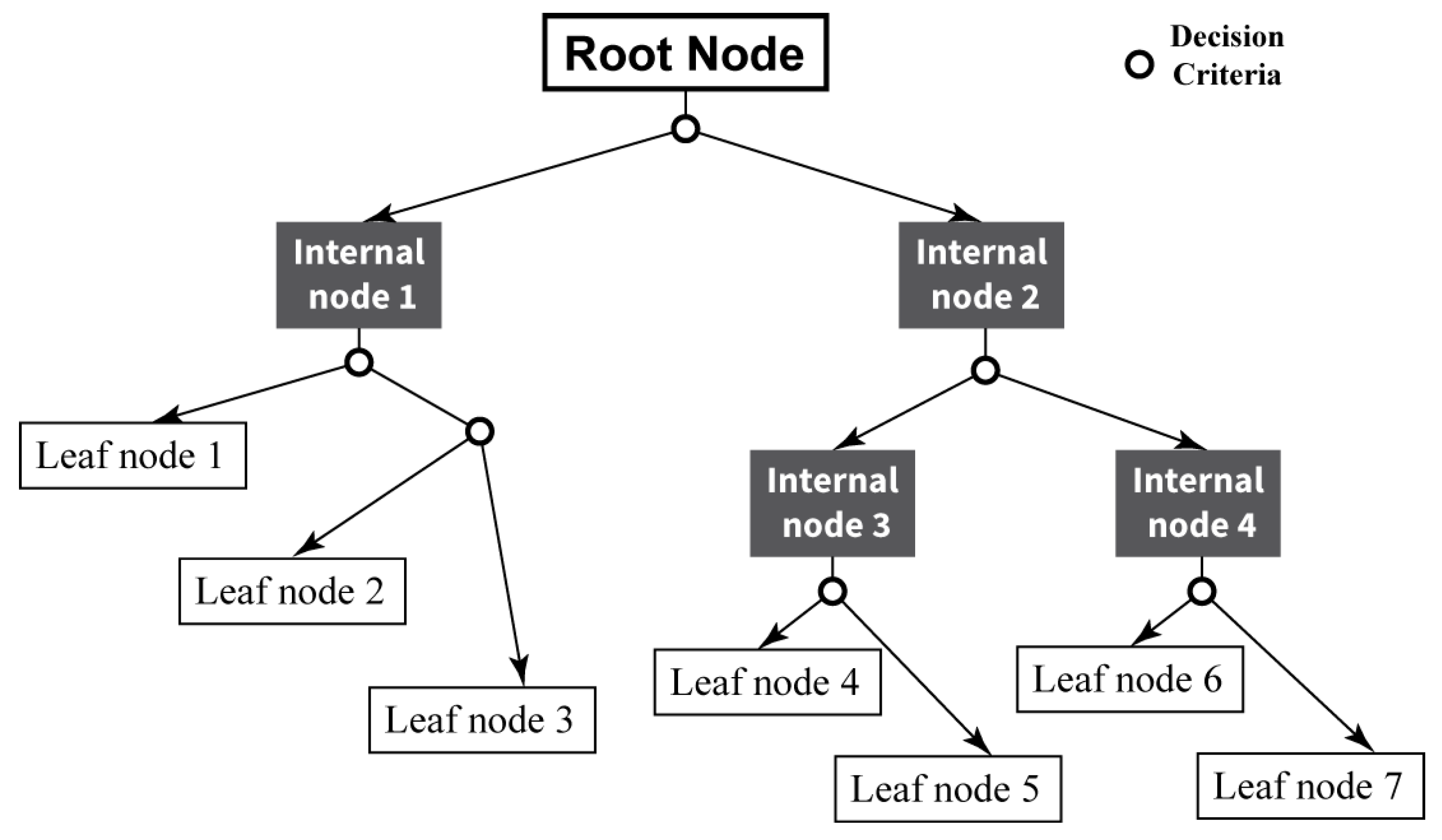
2.1. Principle of CART Algorithm

Decision tree is a widely used data mining method because of its high interpretability [51]. A decision tree model consists of root, internal and leaf nodes. The indicators of a decision tree model for picking branches are information gain, entropy and Gini impurity. Figure 2 shows a schematic diagram of a decision tree model. It uses a top-down recursive method at each node on the sample set to select the branch attribute according to the given criteria from a root node to a leaf node. A leaf node represents an objective function value, which is determined by the input variables along the path from the root node to the leaf node.
Compared to other data mining methods, the decision tree algorithm has some strong points that make it suitable for both classification and regression problems [52]: (1) it is simple to understand and interpret; (2) it is able to process both numerical and categorical data; (3) it requires little data preparation; (4) it can validate a model using statistical tests; (5) it uses a non-statistical approach that makes no assumptions of the training data or prediction residuals; and (6) it performs well with large datasets.
CART algorithms, first proposed by Breiman in 1984 [53,54], is a specific decision tree algorithm that is currently widely used. For classification problems, “Gini impurity” is used as the criteria for choosing branches, while for regression problems, mean squared error (MSE) is used.
Gini impurity represents the probability that a randomly chosen sample is misclassified in the sample set. Gini impurity can be calculated as follows:
G i n i A = 1 k = 1 n P k 2
where A represents node A; n is the number of items in a dataset, i = 1, 2, 3, …, n; and  P k  is the fraction of item i in the set.
For regression problems, the goal of CART is to minimize MSE. MSE represents the difference between the predicted value and the actual value in a leaf node, and the calculation formula is as follows:
M S E = 1 n i = 1 n y i y i ^ 2
where n is the number of items in a dataset, i = 1, 2, 3, …, n y i  is the actual value; and  y i ^  is the predicted value.
The right part of Figure 3 illustrates the procedure of a CART model, which can be referred to in [53,54,55] for details. The CART algorithm has the dual functions of classification and regression, which meets the research needs of this paper.

2.2. Establishment of an Extended CART Algorithm for HVAC Sub-Metering Systems

Previous studies [42,43,44,49] have indicated that electricity consumption of lighting-plug systems in commercial buildings presents periodical changes and is not related to both outdoor weather conditions and indoor occupancy rate. Hence, electricity consumption of lighting plugs follows the same pattern over a year, while that of a HVAC system is seasonal (only in summer and winter). Therefore, during a transition season when the HVAC system is closed, the electricity consumption measured by lighting-plug circuits is all lighting-plug electricity consumption. For these reasons, real-time lighting-plug sub-meter data in transition seasons can be used to train a CART model, which can then be used to predict the lighting-plug sub-meter electricity consumption in air-conditioning seasons. Thus, the electricity consumption of HVAC terminal units in air-conditioning seasons can be calculated by the following equation:
E t e r = E m i x E L c a l
where  E L c a l  is the calculated lighting-plug electricity consumption during an air-conditioning season (kWh);  E m i x  is the mixed electricity consumption of the lighting plug and HVAC terminal units that is directly collected from the sub-metering system(kWh); and  E t e r  is the electricity consumption of the HVAC terminal units (kWh).
This procedure is demonstrated on the left side of Figure 3. The model includes two main modules: (1) the lighting-plug electricity consumption prediction module, and (2) the calculation module for the electricity consumption of HVAC terminal units. The main steps are described in the following sections.

2.2.1. Data Pre-Processing

Data pre-processing consists of data cleaning and data transformation. Data cleaning is an important part of data pre-processing. Due to various faults in data collection, transmission and storage procedures, there are a lot of abnormal values, such as missing value, duplicates and outliers, in sub-metering data. Therefore, the data from sub-meters should be cleaned before training models. In this study, a box graph is used to find abnormal data, and linear interpolation is used to fill the missing data. For the data cleaning process, see [55,56] for details.
Commonly, the measurement intervals of sub-metering data are 1–15 min, and the recorded data are instantaneous power. Therefore, in order to facilitate the use of the model, instantaneous power should be converted to hourly electricity consumption. The calculation is shown in Formula (4):
E = i = 1 60 τ P i × τ 60
where E is the electricity consumption (kWh);  P i  is the instantaneous power (kW); and  τ  is the measurement interval (min).

2.2.2. Input Variable Selection

Because electricity consumption of lighting plugs changes periodically, timestamp features are selected as the input variables of the CART model. Table 2 demonstrates different encoding methods and corresponding symbols of timestamp features.
Features in Table 2 can be combined into different input patterns, as summarized in Table 3. For example, No. 1 means to select D, M, T1 and H1 as the model inputs.
In order to select the best input combinations, a CART model was built for each combination. The coefficient of variability (CV, Equation (5)), the weighted mean absolute percentage error (WMAPE, Equation (6)) and the mean time of multiple calculations are chosen as the criteria to select the best input combinations:
C V = i = 1 N E M i E P i 2 N i = 1 N E M i N
W M A P E = i = 1 N E M i E P i i = 1 N E M i
where  E M i  is the metered electricity consumption of the ith data point (kWh);  E P i  is the predicted electricity consumption of the ith data point (kWh); and N is the total point number of the dataset.

2.2.3. Training Period Selection

This section discusses the training period required for model training. Electricity consumption of the lighting-plug system in a transition season is used for training the CART model, and the data in an air-conditioning season are used for testing. In China, cooling seasons are usually from June to September, while heating seasons occur from December to March in the following year. Therefore, data in April, May, October and November can be used in the training process. Table 4 shows the different training periods discussed in this paper.

2.2.4. Electricity Consumption Prediction of Lighting-Plug System

In this study, the electricity consumption of a lighting-plug system and corresponding timestamp features in a transition season are used to train a CART model. The data in an air-conditioning season are the testing data. CV and WMAPE are chosen to evaluate the prediction results.

2.2.5. Electricity Consumption Calculation of HVAC Terminal Units

The real-time electricity consumption of HVAC terminal units can be calculated by using Equation (3). Similarly, CV and WMAPE are chosen to evaluate the disaggregation results. The relative error is also selected for evaluation, and the calculation formula is as follows:
R E = E M i E P i E M i × 100 %

3. Case Study

The model established in Section 3 is demonstrated and tested in this section. It is applied to two actual buildings in Shanghai where the electricity consumption of HVAC terminal units can be measured directly. Basic facilities and operation information about the two buildings are shown in Table 5.

3.1. Data Pre-Processing

In this part, the raw data are cleaned by removing outliers and divided into a training set and a testing set. Table 6 summarizes the data collected from the two buildings and describes the training data and testing data, respectively. Because the sub-metering system has not been used since 2014, the latest sub-metering data of Building A could not be obtained. Therefore, for Building A, data in 2013 are used in the case study, while for Building B, data in 2021 are used. The training data are then re-organized based on seasons and periods according to Table 4.

3.2. Input Variable Selection

The prediction accuracy of the model for the electricity consumption of the lighting-plug system during air-conditioning on and off time are considered separately. As shown in Table 5, the working period of Building A are from 8:00 to 22:00, and the working period of Building B are from 10:00 to 22:00.
Table 7 and Table 8 list the WMAPE, CV and a multiple-computing-mean time  T  (average time for 1000 runs) for different input combinations. The WMAPE and CV indices are calculated separately for three periods: working hours in the cooling season (WHC), working hours in the heating season (WHH), and non-working hours (NW).
In Table 7, Models No. 1 and 2, No. 3 and 4, and No. 5 and 6 are considered as three groups for the comparative analysis. The comparison results show that in each group, the prediction accuracy in working hours is the same, while in the non-working period, the WMAPE and CV of the models with the input H1 are 3.31% and 4.33%, respectively, which are less than those of the models with the input H2. Additionally, when comparing Models No. 8, 9 and 10, the prediction accuracy is very close, while Model No. 10 has the fastest calculation speed. Therefore, T3 is chosen as the date-type encoding form. The calculation speed of Model No. 11 is the highest with 0.0130 s, but the accuracy is significantly lower than the other models. When the model operates during working hours, the WMAPE and CV values of Model No. 11 exceed 12%, while these two criteria of the other models are all within 5%. Model No. 1 is the most accurate; however, its speed is nearly 14 times slower than Model No. 11. Taking model accuracy and running speed into consideration, Model No. 10 is most suitable for Building A. In summary, the electricity consumption prediction model of the lighting-plug system in Building A is mainly influenced by two variables: date type and hour.
The test results of Building B are displayed in Table 8. The evaluation criteria of the model during the WHC and WHH periods of the two buildings are similar. Additionally, during non-working hours, the model of Building A performs better than that of Building B.
Similar to Building A, the results of Model No. 1 to Model No. 6 indicate that in working hours, the predictive accuracy is similar, while in non-working period, the WMAPE and CV of the models with the input H1 are 12.64% and 17.79%, respectively, which are less than those of the models with the input H2. The WMAPE and CV of Model No. 8, Model No.9 and Model No.10 are close. Compared to the above three models, the performance of Model No. 11 is also satisfactory, and the calculation speed is the fastest. In working hours, the WMAPE values of all models are less than 5% and the CV values of all models are less than 9%. Similar to the results of Building A, Model No. 1 is the most accurate, but the calculation speed is more than six times slower than that of model No. 11. Model No. 7 has no significant advantage in both accuracy and calculation speed. Therefore, when comparing the test results of the 11 models, Model No. 11 has the fastest calculation speed while ensuring predictive accuracy. That means the electricity consumption prediction model of the lighting-plug system in Building B is mainly influenced by hour.

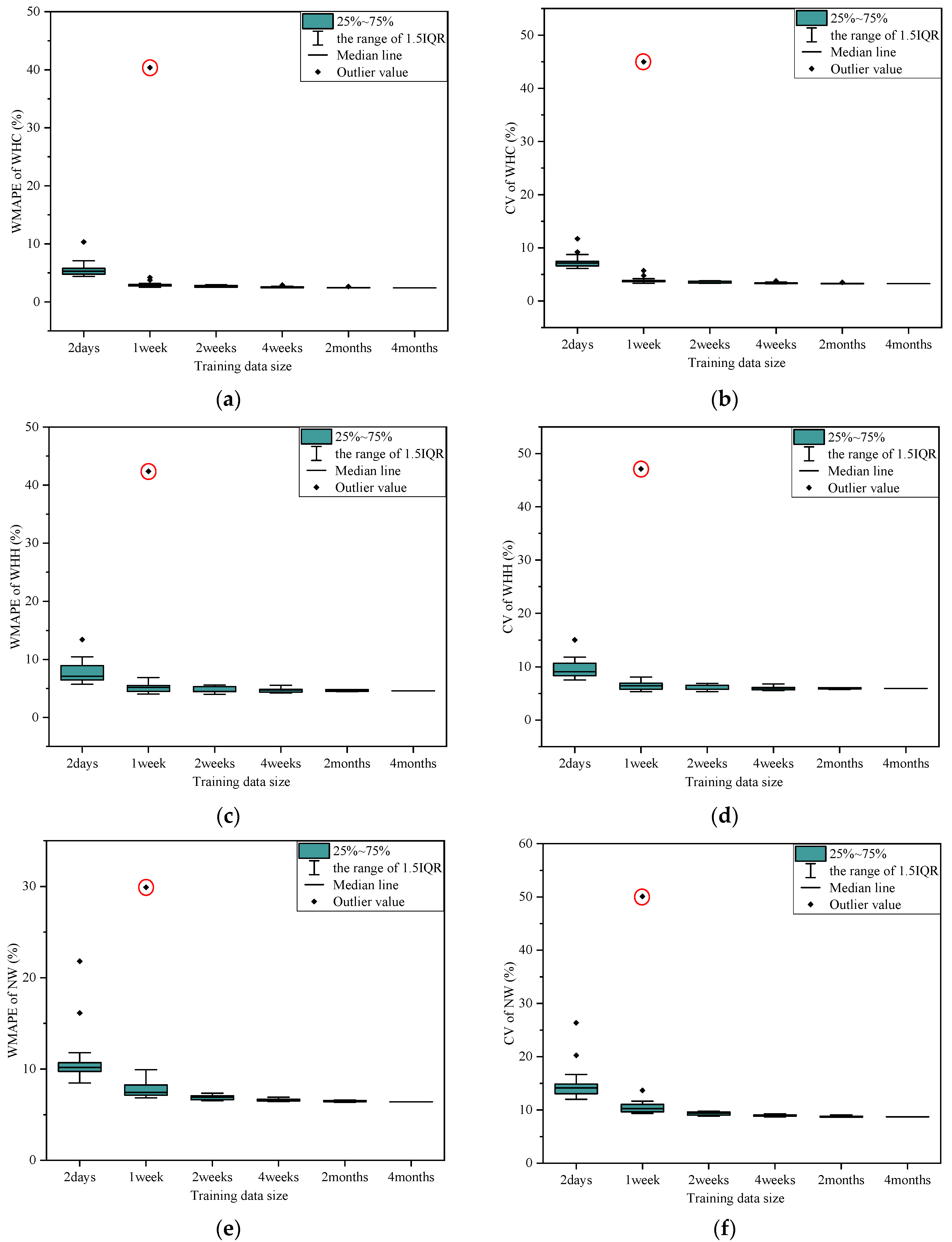
3.3. Training Period Selection

Based on Section 3.2, Model No. 10 is selected for Building A and Model No. 11 is selected for Building B. This section discusses which training period is best for the models in both buildings. The test results of the models with different training periods are shown in Figure 4 and Figure 5. The horizontal axis of the picture refers to the training periods used in the model, and the vertical axis represents the WMAPE and CV of the model with different training periods.
The prediction results for Building A displayed in Figure 4 show that training period has an influence on the accuracy of the model, especially during the NW period. The results shown in (a) and (b) indicate that the model prediction effect during the WHC period is the worst when the 2-day data are used to train the model, and the prediction effects with the other five training periods are close. Figure 4c–e illustrate that during the WHH and NW periods, when the model uses the 1-week and 2-day data as the model training sets, the estimation errors are greater than the errors using the other four training periods. The prediction results of models during the WHC and WHH periods are better than those of the NW period.
In the case of the 1-week training period, there is an outlier shown in the red circle. This is caused by using the data during the National Day Holiday (1 October–7 October 2013) as the training set. The input parameters used by Building A are date type and hour. Since the days during this period are all non-working time, the data in working hours cannot be trained. Thus, the model estimation errors are extremely large.
When the model uses the 2-das data as the training set, there are two outliers in the WMAPE of the model during the NW period. This training set corresponds to the combination of one day in the National Day Holiday and a shift day, which is on a weekend but is shifted to a workday (12 October 2013, Saturday). Due to the existence of holidays and shift days, the electricity consumption of normal workdays shows the features of non-workdays, while the regularity of electricity consumption on normal weekends shows the features of workdays, so the estimation errors of the model is relatively high.
Figure 4 shows that the model can achieve good prediction performance when the training period is four months, two months, four weeks and two weeks. There is no significant difference among these four different periods. Therefore, the 2-week data are selected as the training period for Building A.
Figure 5 shows the estimation errors for Building B. Figure 5a,b show that for WHC, the prediction accuracy of the model trained with the 2-week data is better than the other models. For WHH, as shown in Figure 5c,d, the model with the 2-week training period does not performs well. Figure 5e,f show that the model has the worst prediction accuracy during the NW period, especially when it is trained with the 2-day data. The input variable of Model No. 11 used by Building B is only hour, so other input patterns do not have significant impacts on model accuracy. Since Building B is a shopping mall that is open all year, the building’s electricity consumption does not show significant differences among different date types. Therefore, when the National Day Holiday data are used as the training set, the accuracy of the model in Building B does not decrease significantly. To sum up, the 2-week data are selected as the model training set.

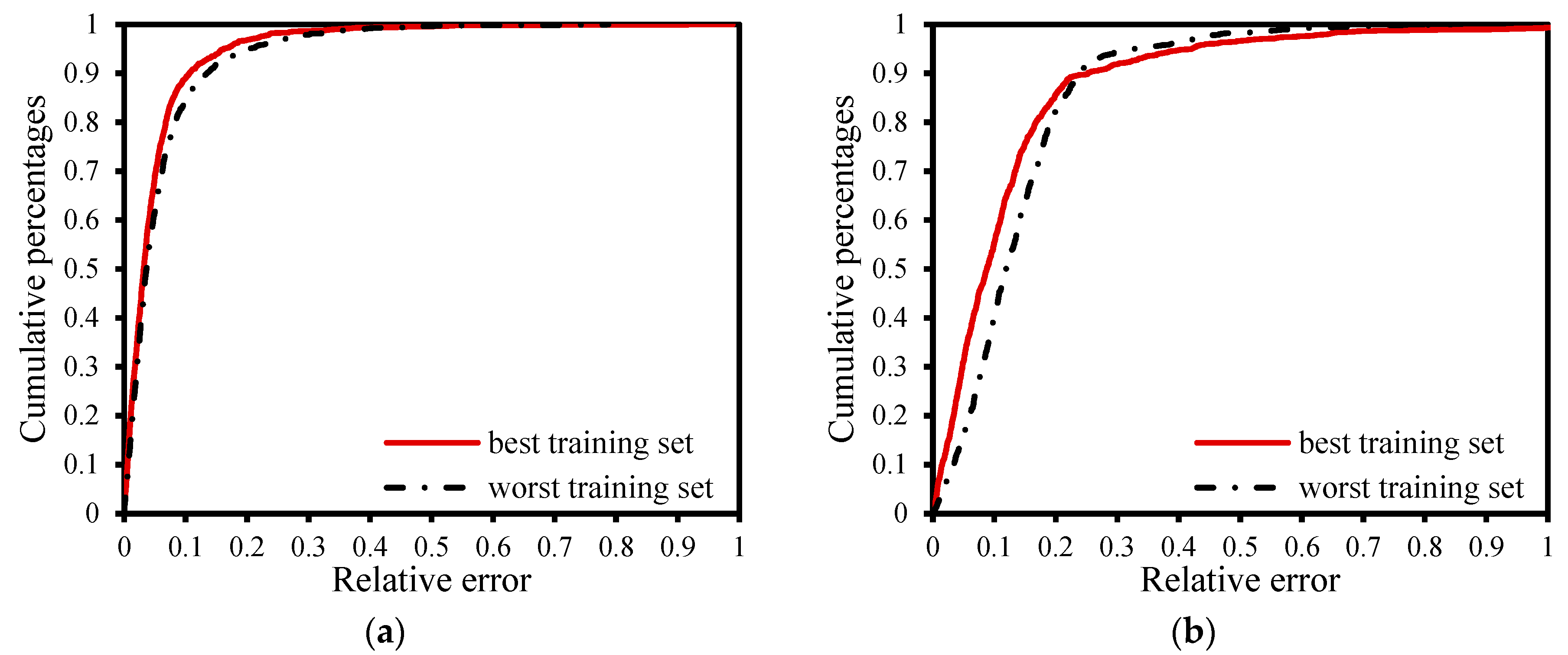
3.4. Electricity Consumption Disaggregation Results of Lighting-Plug System

Based on the results of Section 3.2 and Section 3.3, “T3-H1” is selected as the input combination and the 2-week data are used as the training set for the model in Case A. In Case B, “H1” is selected as the input variable and the 2-week data are used as the training set. In order to verify the accuracy of the model established in this study, the data sets with the best performance and the worst performance are selected to predict the hourly electricity consumption of the lighting-plug system separately. In Case A, the training set with the best performance is from 1 November to 14 November 2013, and the training set with the worst performance is from 15 April to 28 April 2013. In Case B, the training set with the best performance is from 18 May to 31 May 2021, and the training set with the worst performance is from 6 April to 19 April 2021.
Table 9 shows the model performance of Building A and Building B. For Case A, the WMAPE values of the best performance model during the WHC, WHH and NW are 2.50%, 4.42% and 6.59%, and the CV values are 3.35%, 5.75 % and 9.11%, respectively. The WMAPE values of the worst performance model during the WHC, WHH and NW are 2.94%, 5.62% and 7.15%, and the CV values are 3.82%, 6.87% and 9.75%, respectively. For Case B, the best WMAPE values during the WHC, WHH and NW are 2.57%, 4.81% and 16.00%, and the best CV values are 8.59%, 8.23% and 24.13%, respectively, while the worst WMAPE values are 5.55%, 4.89% and 21.09%, and the worst CV values are 8.27%, 8.54% and 27.23%, respectively.

3.5. Electricity Consumption Calculation of HVAC Terminal Units

This section verifies the accuracy of the method proposed in this research to predict the hourly electricity consumption of HVAC terminal units. The model disaggregation results of the best training set for the two buildings are shown in Figure 6. Additionally, Table 10 summarizes the WMAPE and CV values of the electricity consumption disaggregation results of the HVAC terminal units in the two buildings. Figure 7 and Figure 8 show the probability cumulative curves of the relative error of all data points.
In Figure 6, the red dots are actual electricity consumption of the HVAC terminal units during working hours in the two buildings, while the black crosses indicate the electricity consumption during working hours predicted by the CART model established in this study. It can be seen that the predicted values change consistently with the actual values.
For Building A, the minimum WMAPE values during the WHC, WHH and NW are 3.79%, 10.05% and 21.90%, and the minimum CV values are 5.09%, 13.07% and 30.26%, respectively, while the maximum WMAPE values during the WHC, WHH and NW are 4.47%, 12.76% and 23.75%, and the maximum CV values are 5.80%, 15.60% and 32.39%, respectively.
The probability cumulative curve of the samples at different relative error levels is shown in Figure 7. There are 1274 testing samples for the cooling season and 1227 testing samples for the heating season. During the WHC, the cumulative percentage of samples with a relative error lower than 15% is 93.7% when using the best training set, while it is 91.7% when using the worst training set. During the WHH, for the best data set, 75.6% of the samples’ relative errors are less than 15% and more than 91.8% of the samples’ relative errors are less than 30%. For the worst data set, 63.9% of the samples’ relative errors are less than 15% and 93.9% of the samples’ relative errors are less than 30%. Considering Table 10 and Figure 7 comprehensively, the following conclusions can be drawn for Case A: (A1) models with the best and the worst training sets have little difference; (A2) the disaggregation accuracy for the cooling season is better than the heating season; and (A3) the predication accuracy for working hours is much better than non-working hours.
Similarly, for Building B, the minimum WMAPE values during the WHC, WHH and NW are 2.25%, 8.34% and 6.47%, and the minimum CV values are 7.54%, 14.28% and 9.75%, respectively. The maximum WMAPE values during the WHC, WHH and NW are 2.24%, 8.48% and 5.83%, and the maximum CV values are 7.50%, 14.35% and 11.01%, respectively.
The number of testing samples for Case B is 1586 in the cooling season and 1573 in the heating season. For the model with the best training set, the proportion of the samples with relative errors less than 15% is 99.1% (during WHC) and 83.8% (during WHH). For the model with the worst training set, this proportion is 99.1% (during WHC) and 83.4% (during WHH), respectively. The conclusions for Case B are as follows: (B1) during the WHC and WHH, the disaggregation resluts of these two models are similar; (B2) the model accuracy in the cooling season is better than that in the heating season; and (B3) the disaggregation accuracy of WHC and non-working hours are better than WHH.

4. Discussion

Based on the results of the two case studies, the application effects of the proposed disaggregation method are further discussed in this section.
The time schedule input pattern of Building A is optimized as “T3-H1” and that for Building B is “H1”. This means that the model of Building A uses "Date Type" and "Hour" as the input variables, and the model of Building B only uses "Hour". Building A is a complex commercial building with both office and shopping areas, while Building B is purely a shopping mall. Thus, for buildings with office area, "Date Type" should be taken into consideration because the occupancy pattern on weekdays, weekends and holidays are quite different. Lighting system is usually off on weekends and holidays. However, for shopping malls, lighting systems follow the same pattern. Only "Hour" is used as the input.
By comparing the changes in model prediction accuracy under different training sets, it is determined that the amount of training data required for the two buildings are same. A 2-week data set can be used to train the models.
Based on the conclusions (A2) and (B2) drawn in Section 3.5, the disaggregation accuracy in the cooling season is better than in the heating season. During the WHC, the disaggregation accuracy of the model in two buildings are similar, while during the WHH, the disaggregation accuracy of the model in Building B is higher than that in Building A. The on-site survey results show that some other types of heating facilities (such as electric heaters) are occasionally used during the heating season in Building A, which affects the energy consumption regularity of the lighting-plug system to some extent. For example, some staff use electric heaters in the office when it is too cold in winter. This phenomenon incidentally affects the accuracy of the hourly electricity use calculation of the lighting-plug system and HVAC terminal units. Therefore, the disaggregation accuracy in the cooling season is better than in the heating season.
Based on the conclusions (A3) drawn in Section 3.5, the result for working hours is much better than that for non-working hours. One reason is that the electricity consumption of HVAC terminal units is very small during non-working hours. A little difference could cause large WMAPE and CV errors. Another reason is that during working hours, occupants have formed a certain behavior pattern and the lighting systems are generally turned on. However, during non-working hours, occupant behaviors are quite random. For example, sometimes some people would work overtime. It is difficult to accurately predict the electricity consumption of the HVAC terminal units caused by these random occupant behaviors. Compared to the electricity consumption of the HVAC terminal units during working hours, the consumption during non-working hours only accounts for a little part of the operating electricity consumption of the HVAC terminal units. Thus, the disaggregation results in working hours are more importance in practice.
Generally, the HVAC system keeps off during non-working hours. However, the hourly electricity consumption of the HVAC terminal units in non-working hours is still considered in this research. Our purpose is to monitor the operating schedule of the HVAC terminals using the calculated energy data. For example, if energy use appears during non-working time, it indicates that some HVAC terminal units may not be closed.

5. Conclusions

In order to solve the mismatch problem of sub-metering systems in public buildings, this research proposes a disaggregation method based on a CART algorithm. This method performs well in two buildings in Shanghai.
The main conclusions of this study are as follows: (1) Considering the prediction accuracy and running time of the model, T3-H1 is selected as the input parameter for the office–shopping mall complex building (Building A), and H1 is selected for the shopping mall (Building B). (2) The impact of date type on electricity consumption of office buildings is more significant than shopping malls. (3) The 2-week data set can meet the model accuracy requirements. (4) For the hourly electricity consumption disaggregation result of the HVAC terminal units in Building A, the minimum WMAPE values of WHC and WHH are 3.79% and 10.05%, and the minimum CV values are 5.09% and 13.07%, respectively. For Building B, the minimum WMAPE values of WHC and WHH are 2.25% and 8.34%, and the minimum CV values are 7.54% and 14.28%, respectively.
The advantages of this proposed method are the following: (1) It is simple and convenient to applied. The input variables in the model just need time features, which are all very easy to obtain and sufficient to support the model accuracy. According to the case study results, two-week data are enough for training a model, so it is very convenient in practical application. (2) This method is versatile. Although there are only two case studies in this paper, this method can be used in other buildings to disaggregate seasonal sub-metering data with non-seasonal sub-metering data.
The limitations of this proposed method are the following: (1) This method can only disaggregate seasonal data from non-seasonal data. It cannot disaggregate the electricity consumption of equipment or devices with the same operation patterns. (2) Other features, such as weather and occupant behaviors, can be taken into consideration in future works.

Author Contributions

Conceptualization, Y.J.; Software, X.Y. and Y.J.; Validation, X.Y.; Formal analysis, M.N.; Investigation, J.G.; Resources, Y.J.; Writing—original draft, Y.J.; Writing—review & editing, X.Y. and J.G.; Visualization, X.Y.; Funding acquisition, Y.J. All authors have read and agreed to the published version of the manuscript.

Funding

This study was funded by the Youth Program of National Natural Science Foundation of China (No. 51908006).

Data Availability Statement

Not applicable.

Conflicts of Interest

The authors declare no conflict of interest.

Abbreviations

HVACHeating, Ventilation and Air Conditioning
VAVVariable Air Volume System
CARTClassification and Regression Tree
NILMNon-intrusive Load Monitoring
EDAEnd-use Disaggregation Algorithm
ANNArtificial Neural Network
GiniGini Impurity
CVCoefficient of Variability
WMAPEWeighted Mean Absolute Percentage Error
WHCWorking Hours in Cooling Season
WHHWorking Hours in Heating Season
NWNon-working Hours
EL_calCalculated lighting-plug electricity consumption in the air conditioning season (kWh)
EmixMixed electricity consumption of the lighting plug and HVAC terminal units (kWh)
EterElectricity consumption of terminal units in the air conditioning system (kWh)
EElectricity consumption (kWh)
PiInstantaneous power (kW)
τCount cycle of instantaneous power (min).
DDays in one year
MMonths from January to December
TDate types
HEquipment use time
EMiMetered electricity consumption of the ith data point (kWh)
EpiPredicted electricity consumption of the ith data point (kWh)
NTotal point number of the dataset
  T Multiple-computing-mean time (s)

References

  1. IEA. Buildings: IEA, Paris. License: CC BY 4.0. 2022. Available online: https://www.iea.org/reports/buildings (accessed on 10 December 2022.).
  2. Building Energy Conservation Research Center of Tsinghua University. Annual Report on China Building Energy Efficiency 2022; Building Energy Conservation Research Center of Tsinghua University: Beijing, China, 2022. [Google Scholar]
  3. Hart, G.W. Nonintrusive appliance load monitoring. Proc. IEEE 1992, 80, 1870–1891. [Google Scholar]
  4. Howard, E. California. Guide to the Implementation of Tenant Submetering and Billing for Commercial Buildings in Northern California; SILO Inc.: Brooklyn, NY, USA, 2008. [Google Scholar]
  5. Ministry of Finance of the People's Republic of China. Interim Measures for the Administration of Special Funds for Energy Saving of State-owned Buildings and Large-scale Public Buildings; Document No. 5582007; Ministry of Finance of the People's Republic of China: Beijing, China, 2007.
  6. Junruo, W. Case analysis on energy consumption of large-scale public buildings in shanghai area based on partial subentry measurement system. New Build. Mater. 2010, 37, 48–50. [Google Scholar]
  7. Zhang, H.W.Q.; Li, Y.; Wang, X. Research and development on electricity sub-metering system for large public buildings (Part Ⅰ): System structure. Heat. Vent. Air Cond. 2010, 40, 10–13+50. [Google Scholar]
  8. Wang, X.W.Q.; Shen, Q.; Zhang, H. Research and development on electricity sub-metering system for large public buildings (Part Ⅱ): Uniform model and methodology of energy consumption classification. Heat. Vent. Air Cond. 2010, 40, 14–17. [Google Scholar]
  9. Tongji University BEAD. Building Energy Consumption Sub-metering Data Status and Application Seminar; Tongji University BEAD: Shanghai, China, 2016. [Google Scholar]
  10. Ministry of Housing and urban-rural development of the People’s Republic of China. Technical Guideline for Sub-Metering Data Collection of Energy Consumption Monitoring System in State-Owned Buildings and Large-Scale Public Buildings; Document No. 114; Ministry of Housing and urban-rural development of the People’s Republic of China: Beijing, China, 2008.
  11. Qu, Y.; Zhang, Z.; Wang, H.; Yang, F. Energy Consumption Analysis of Public Buildings Located in the Severe Cold Region. Procedia Eng. 2017, 205, 2111–2117. [Google Scholar]
  12. Guo, C.; Bian, C.; Liu, Q.; You, Y.; Li, S.; Wang, L. A new method of evaluating energy efficiency of public buildings in China. J. Build. Eng. 2022, 46, 103776. [Google Scholar]
  13. Sizirici, B.; Fseha, Y.; Cho, C.-S.; Yildiz, I.; Byon, Y.-J. A Review of Carbon Footprint Reduction in Construction Industry, from Design to Operation. Materials 2021, 14, 6094. [Google Scholar] [CrossRef]
  14. Granderson, J.; Lin, G.; Singla, R.; Fernandes, S.; Touzani, S. Field evaluation of performance of HVAC optimization system in commercial buildings. Energy Build. 2018, 173, 577–586. [Google Scholar] [CrossRef]
  15. Marceau, M.; Zmeureanu, R. Nonintrusive load disaggregation computer program to estimate the energy consumption of major end uses in residential buildings. Energy Convers. Manag. 2000, 41, 1389–1403. [Google Scholar] [CrossRef] [Green Version]
  16. Laughman, C.; Lee, K.; Cox, R.; Shaw, S.; Leeb, S.; Norford, L.; Armstrong, P. Power signature analysis. IEEE Power Energy Mag. 2003, 1, 56–63. [Google Scholar]
  17. Giri, S.; Bergés, M. An energy estimation framework for event-based methods in Non-Intrusive Load Monitoring. Energy Convers. Manag. 2015, 90, 488–498. [Google Scholar] [CrossRef]
  18. Murata, H.; Onoda, T. Estimation of power consumption for household electric appliances. In Proceedings of the Conference Estimation of Power Consumption for Household Electric Appliances, Singapore, 18–22 November 2002; Volume 5, pp. 2299–2303. [Google Scholar]
  19. Liu, Q.; Nakoty, F.M.; Wu, X.; Anaadumba, R.; Liu, X.; Zhang, Y.; Qi, L. A secure edge monitoring approach to unsupervised energy disaggregation using mean shift algorithm in residential buildings. Comput. Commun. 2020, 162, 187–195. [Google Scholar] [CrossRef]
  20. Dash, S.; Sahoo, N. Electric energy disaggregation via non-intrusive load monitoring: A state-of-the-art systematic review. Electr. Power Syst. Res. 2022, 213, 108673. [Google Scholar] [CrossRef]
  21. Norford, L.K.; Mabey, N. Non-Intrusive Electric Load Monitoring in Commercial Buildings. Symposium on Improving Building Systems in Hot and Humid Climates; Texas A&M University: College Station, TX, USA, 1992. [Google Scholar]
  22. Norford, L.K.; Leeb, S.B. Non-intrusive electrical load monitoring in commercial buildings based on steady-state and transient load-detection algorithms. Energy Build. 1996, 24, 51–64. [Google Scholar] [CrossRef]
  23. Rafsanjani, H.N.; Ahn, C. Linking Building Energy-Load Variations with Occupants’ Energy-Use Behaviors in Commercial Buildings: Non-Intrusive Occupant Load Monitoring (NIOLM). Procedia Eng. 2016, 145, 532–539. [Google Scholar] [CrossRef] [Green Version]
  24. Rafsanjani, H.N.; Ahn, C.R.; Chen, J. Linking building energy consumption with occupants’ energy-consuming behaviors in commercial buildings: Non-intrusive occupant load monitoring (NIOLM). Energy Build. 2018, 172, 317–327. [Google Scholar] [CrossRef]
  25. Kaselimi, M.; Doulamis, N.; Doulamis, A.; Voulodimos, A.; Protopapadakis, E. Bayesian-optimized Bidirectional LSTM Regression Model for Non-intrusive Load Monitoring. In Proceedings of the ICASSP 2019–2019 IEEE International Conference on Acoustics, Speech and Signal Processing (ICASSP), Brighton, UK, 12–17 May 2019; pp. 2747–2751. [Google Scholar]
  26. Schirmer, P.A.; Mporas, I.; Paraskevas, M. Evaluation of Regression Algorithms and Features on the Energy Disaggregation Task. In Proceedings of the 2019 10th International Conference on Information, Intelligence, Systems and Applications (IISA), Patras, Greece, 15–17 July 2019; pp. 1–4. [Google Scholar]
  27. Kaselimi, M.; Protopapadakis, E.; Voulodimos, A.; Doulamis, N.; Doulamis, A. Multi-Channel Recurrent Convolutional Neural Networks for Energy Disaggregation. IEEE Access 2019, 7, 81047–81056. [Google Scholar] [CrossRef]
  28. Yang, D.; Gao, X.; Kong, L.; Pang, Y.; Zhou, B. An Event-Driven Convolutional Neural Architecture for Non-Intrusive Load Monitoring of Residential Appliance. IEEE Trans. Consum. Electron. 2020, 66, 173–182. [Google Scholar] [CrossRef]
  29. Faustine, A.; Pereira, L.; Bousbiat, H.; Kulkarni, S. UNet-NILM: A Deep Neural Network for Multi-Tasks Appliances State Detection and Power Estimation in NILM. In Proceedings of the 5th International Workshop on Non-Intrusive Load Monitoring NILM’20 Association for Computing Machinery, New York, NY, USA, 18 November 2020; pp. 84–88. [Google Scholar]
  30. Xia, M.; Liu, W.; Wang, K.; Song, W.; Chen, C.; Li, Y. Non-intrusive load disaggregation based on composite deep long short-term memory network. Expert Syst. Appl. 2020, 160, 113669. [Google Scholar] [CrossRef]
  31. Guo, Y.; Xiong, X.; Fu, Q.; Xu, L.; Jing, S. Research on non-intrusive load disaggregation method based on multi-model combination. Electr. Power Syst. Res. 2021, 200, 107472. [Google Scholar] [CrossRef]
  32. Monteiro, R.; de Santana, J.; Teixeira, R.; Bretas, A.; Aguiar, R.; Poma, C. Non-intrusive load monitoring using artificial intelligence classifiers: Performance analysis of machine learning techniques. Electr. Power Syst. Res. 2021, 198, 107347. [Google Scholar] [CrossRef]
  33. Samadi, M.; Fattahi, J. Energy use intensity disaggregation in institutional buildings—A data analytics approach. Energy Build. 2021, 235, 110730. [Google Scholar] [CrossRef]
  34. Xiao, Z.; Gang, W.; Yuan, J.; Zhang, Y.; Fan, C. Cooling load disaggregation using a NILM method based on random forest for smart buildings. Sustain. Cities Soc. 2021, 74, 103202. [Google Scholar] [CrossRef]
  35. Athanasiadis, C.; Doukas, D.; Papadopoulos, T.; Chrysopoulos, A. A Scalable Real-Time Non-Intrusive Load Monitoring System for the Estimation of Household Appliance Power Consumption. Energies 2021, 14, 767. [Google Scholar] [CrossRef]
  36. Shao, H.; Marwah, M.; Ramakrishnan, N. A Temporal Motif Mining Approach to Unsupervised Energy Disaggregation: Applications to Residential and Commercial Buildings. Proc. Conf. AAAI Artif Intell 2013, 27, 1327–1333. [Google Scholar] [CrossRef]
  37. Burak, G.H.; Shi, Z.; Wilton, I.; Bursill, J. Disaggregation of commercial building end-uses with automation system data. Energy Build. 2020, 223, 110222. [Google Scholar]
  38. Zaeri, N.; Ashouri, A.; Gunay, H.B.; Abuimara, T. Disaggregation of electricity and heating consumption in commercial buildings with building automation system data. Energy Build. 2021, 258, 111791. [Google Scholar] [CrossRef]
  39. Elafoudi, G.; Stankovic, L.; Stankovic, V. Power disaggregation of domestic smart meter readings using dynamic time warping. In Proceedings of the Conference Power Disaggregation of Domestic Smart Meter Readings Using Dynamic Time Warping, Athens, Greece, 21–23 May 2014; pp. 36–39. [Google Scholar]
  40. Kolter, J.Z.; Batra, S.; Ng, A.Y. Energy Disaggregation via Discriminative Sparse Coding. In Proceedings of the 23rd International Conference on Neural Information Processing Systems, Vancouver, Canada, 6–9 December 2010; Volume 1, pp. 1153–1161. [Google Scholar]
  41. Matsui, K.; Yamagata, Y.; Nishi, H. Disaggregation of Electric Appliance’s Consumption Using Collected Data by Smart Metering System. Energy Procedia 2015, 75, 2940–2945. [Google Scholar]
  42. Dhar, A.; Reddy, T.A.; Claridge, D.E. A Fourier Series Model to Predict Hourly Heating and Cooling Energy Use in Commercial Buildings with Outdoor Temperature as the Only Weather Variable. J. Sol. Energy Eng. 1999, 121, 47–53. [Google Scholar] [CrossRef]
  43. Dhar, A.; Reddy, T.A.; Claridge, D.E. Modeling Hourly Energy Use in Commercial Buildings with Fourier Series Functional Forms. J. Sol. Energy Eng. 1998, 120, 217–223. [Google Scholar] [CrossRef]
  44. Dhar, A.; Reddy, T.A.; Claridge, D.E. Generalization of the Fourier Series Approach to Model Hourly Energy Use in Commercial Buildings. J. Sol. Energy Eng. 1999, 121, 54–62. [Google Scholar] [CrossRef]
  45. Ji, Y.; Xu, P.; Ye, Y. HVAC terminal hourly end-use disaggregation in commercial buildings with Fourier series model. Energy Build. 2015, 97, 33–46. [Google Scholar] [CrossRef]
  46. Fan, C.; Wang, J.; Gang, W.; Li, S. Assessment of deep recurrent neural network-based strategies for short-term building energy predictions. Appl. Energy 2018, 236, 700–710. [Google Scholar] [CrossRef]
  47. Parzen, E.; Pandit, S.M.; Wu, S.-M. Time Series and System Analysis with Applications. J. Am. Stat. Assoc. 1985, 80, 251. [Google Scholar] [CrossRef]
  48. Braun, J.E. Performance and control characteristics of a large cooling system. ASHRAE Trans. 1987, 93, 1830–1852. [Google Scholar]
  49. Claridge, D.E.; Haberl, J.S.; Turner, D.; O'Neal, D.L.; Jaeger, S. Improving energy conservation retrofits with measured savings. ASHRAE J. 1991, 33, 10–14. [Google Scholar]
  50. Ji, Y.; Xu, P. A bottom-up and procedural calibration method for building energy simulation models based on hourly electricity submetering data. Energy 2015, 93, 2337–2350. [Google Scholar] [CrossRef]
  51. Lior, R.; Maimon, O. Data Mining with Decision Trees: Theory and Applications; World Scientific Publishing Co. Inc.: Singapore, 2007. [Google Scholar]
  52. James, G.; Witten, D.T.H. An Introduction to Statistical Learning; Springer: New York, NY, USA, 2013; Volume 103, pp. 78–129. [Google Scholar]
  53. Breiman, L.; Friedman, J.R.O.; Stone, C. Classification and Regression Trees; Wadsworth International Group: Belmont, CA, USA, 1984; Volume 40, pp. 17–23. [Google Scholar]
  54. Breiman, L.; Friedman, J.H.R.O. Classification and Regression Trees. Wadsworth & Brooks. J. Am. Stat. Association. 1984, 18, 358. [Google Scholar]
  55. Wang, H.; Xu, P.; Lu, X.; Yuan, D. Methodology of comprehensive building energy performance diagnosis for large commercial buildings at multiple levels. Appl. Energy 2016, 169, 14–27. [Google Scholar] [CrossRef]
  56. Fu, Y.; Li, Z.; Feng, F.; Xu, P. Data-quality detection and recovery for building energy management and control systems: Case study on submetering. Sci. Technol. Built Environ. 2016, 22, 798–809. [Google Scholar] [CrossRef]
Figure 1. Structure of a sub-metering system and the gap between an actual model and the theoretical classification model.
Buildings 13 00967 g001
Figure 2. Schematic diagram of a decision tree model.
Buildings 13 00967 g002
Figure 3. The establishment procedure of a CART model.
Buildings 13 00967 g003
Figure 4. Case A test results with different training data sizes: (a) the range of WMPE varies during the WHC; (b) the range of CV varies during the WHC; (c) the range of WMPE varies during the WHH; (d) the range of CV varies during the WHH; (e) the range of WMPE varies during the NW; and (f) the range of CV varies during the NW.
Buildings 13 00967 g004
Figure 5. Test results of Building B with different training periods: (a) the range of WMPE varies during the WHC; (b) the range of CV varies during the WHC; (c) the range of WMPE various during the WHH; (d) the range of CV various during the WHH; (e) the range of WMPE various during the NW; and (f) the range of CV various during the NW.
Buildings 13 00967 g005
Figure 6. Energy consumption disaggregation results of HVAC terminal units: (a) Building A with the best training set, and (b) Building B with the best training set.
Buildings 13 00967 g006
Figure 7. Building A: the probability cumulative curve of the samples at different relative error levels. (a) Cooling season. (b) Heating season.
Buildings 13 00967 g007
Figure 8. Building B: the probability cumulative curve of the samples at different relative error levels. (a) Cooling season. (b) Heating season.
Buildings 13 00967 g008
Table 1. Summary of existing NILM methods.
No.AuthorMethodBuilding TypeInputsOutputReference
1Rafsanjani et al.Machine learningCommercial buildingOccupant, minimum numbers of data points, entry events, and departure eventsOccupants’ power changes[23,24]
2Kaselimi et al.Machine learningResidential buildingAggregate energy signals over a time windowThe consumption of electric appliances[25]
3Schirmer et al.Machine learningResidential buildingStatistical features, line currents, line voltages, and load anglesThe consumption of electric appliances[26]
4Kaselimi MMachine learningResidential buildingCurrent, active power, reactive power, and apparent powerThe current state of appliances[27]
5Yang DMachine learningResidential buildingCharacteristics of residential applianceThe consumption of electric appliances[28]
6Faustine AMachine learningResidential buildingAggregate power signal and power signalsThe consumption of electric appliances[29]
7Xia et al.Machine learningResidential buildingOriginal main power data and differential processing dataThe consumption of electric appliances[30]
8Guo et al.Machine learningResidential buildingTwo-phase current cycle changes, single-phase voltage cycle changes, and apparent power changesThe consumption of electric appliances[31]
9Monteiro et al.Machine learningResidential buildingNumber of connected devices, number of device combinations, and labelled current waveformsThe consumption of electric appliances[32]
10SamadiMachine learningInstitutional buildingAmbient temperature, workday, time of day, daylight length, intensity of sunlight, number of occupants, and humidityCommon and occupancy loads, and exterior and interior lighting[33]
11Xiao et al.Machine learningOffice buildingTotal load, outdoor weather or coefficients of Fourier for total loadOccupant load, building envelope load, fresh air load, and equipment load.[34]
12Athanasiadis CMachine learningResidential buildingActive power transient responseActive power of appliances[35]
13Shao et al.Temporal motif miningResidential buildingAggregated power observation time seriesThe disaggregated time series for each device[36]
14Burak Gunay et al.Regression modelCommercial buildingAHU schedule, outdoor temperature, AHU fan state, chiller pump state, AHU supply air pressure, AHU schedule Occupant-controlled loads, scheduled distribution loads, and cooling loads[37]
15Zaeri et al.Regression modelCommercial buildingDischarge airflow rate for AHUs and occupancy dataOccupant-controlled loads and distribution loads[38]
16Elafoudi et al.Dynamic time warpingResidential buildingAggregate active power data and a library of signatures for expert classificationThe name of appliances, and the timestamp of the event[39]
17Kolter et al.Sparse codingResidential buildingWhole home signal and models of each device’s electricity consumptionThe consumption of electric appliances[40]
18Matsui et al.Sparse codingResidential buildingModel of each electric appliance’s electricity consumption over a weekThe consumption of electric appliances[41]
19Ji et al.Fourier seriesCommercial buildingSub-metering dataThe energy consumption of HVAC terminals[45]
Table 2. Summary of symbols and encoding methods of timestamp features.
FeatureSymbolCodeExplanation
DateD1–365 (or 366)Days in one year
MonthM1–12Months from January to December
Date TypeT10–8Monday–Sunday (1–7), holiday (8), and compensated workday (0).
T20–2Weekday (1), weekend (0), and holiday (2)
T30–1Workday (1) and non-workday (0)
HourH10–24Hours in one day
H28–17, 0For office building, service hours (8:00–17:00) are labeled as 8–17, other hours (0)
10–22, 0For shopping mall, service hours (10:00–22:00) are labeled as 10–22, other hours (0)
8–22, 0For office–shopping complex building service hours (8:00–22:00) are labeled as 8–22, other hours (0)
——The special serve time is adjusted according to the actual building information
Table 3. Summary of different schedule input combinations.
No.Input Combination
1D-M-T1-H1
2D-M-T1-H2
3D-M-T2-H1
4D-M-T2-H2
5D-M-T3-H1
6D-M-T3-H2
7M-T1-H1
8T1-H1
9T2-H1
10T3-H1
11H1
Table 4. Summary table of the training data size selection.
No.Training PeriodDescription
14 monthswhole transition season data
22 months1-month data in spring and 1-month data in fall
34 weeks2-week data in spring and 2-week data in fall
42 weeks2-week data in transition season
51 week1-week data in transition season
62 days1-workday data and 1-non-workday data
Table 5. Structural information for the two buildings in Shanghai used in this study.
Building NameBuilding ABuilding B
CityShanghaiShanghai
Building typeComplex buildingShopping mall
FloorsShopping mall (1–4) and offices (5–34)9
Area (m2)68,33040,000
Service timeShopping mall: Full year 10:00–22:00;
Office: Weekdays 8:00–18:00
Full year: 10:00–22:00
HVAC terminal unitsAHU (shopping mall) and FCU+FAU (office)AHU
Energy typeElectricElectric
Table 6. Selected electrical input data from two buildings studied in Shanghai.
Building NameData of Lighting-Plug SystemTraining DataTesting Data
Data of Transition SeasonData of HVAC Terminal Units
Cooling SeasonHeating Season
A1 January–31 December 20131 April–31 May
1 October–30 November
1 June–30 September1 January–31 March
1 December–31 December
B1 January–31 December 20211 April–31 May
1 October–30 November
1 June–30 September1 January–31 March
1 December–31 December
Table 7. Test results for lighting-plug system in different schedule input patterns in Case A.
Model No.Input CombinationWMAPE (%)CV (%)   T  (s)
WHCWHHNWWHCWHHNW
1D-M-T1-H11.001.221.891.391.912.750.1780
2D-M-T1-H21.001.225.201.391.917.080.1432
3D-M-T2-H11.091.182.821.501.794.580.2503
4D-M-T2-H21.091.186.091.501.797.940.1892
5D-M-T3-H11.091.182.881.491.794.580.2090
6D-M-T3-H21.091.186.131.491.797.950.1706
7M-T1-H11.551.883.382.182.815.060.1394
8T1-H12.303.344.572.994.606.560.0195
9T2-H12.383.485.963.164.848.300.0148
10T3-H12.383.486.253.164.848.650.0140
11H112.2814.0222.8215.4218.2337.310.0130
Table 8. Test results for lighting-plug system in different schedule input patterns in Case B.
Model No.Input CombinationWMAPE (%)CV (%)   T  (s)
WHCWHHNWWHCWHHNW
1D-M-T1-H10.820.748.152.901.0712.410.0529
2D-M-T1-H20.820.7420.792.901.0732.200.0970
3D-M-T2-H10.820.757.932.901.0911.990.0508
4D-M-T2-H20.820.7520.802.901.0932.200.0809
5D-M-T3-H10.830.757.882.911.0811.950.0544
6D-M-T3-H20.830.7520.792.911.0832.200.0893
7M-T1-H12.221.5811.836.975.5518.460.0653
8T1-H13.264.0716.477.548.7523.310.0127
9T2-H13.174.0516.538.887.5123.500.0098
10T3-H13.164.0816.418.847.7123.560.0101
11H13.144.0916.488.847.7723.590.0084
Table 9. The input parameters, training periods and disaggregation estimation errors of the model in Case A and Case B.
CaseInput PatternTraining Data Size and PerformanceWMAPE (%)CV (%)
WHCWHHNWWHCWHHNW
AT3-H12 weeks (best)
(1 November–14 November 2013)
2.504.426.593.355.759.11
2 weeks (worst)
(15 April–28 April 2013)
2.945.627.153.826.879.75
BH12 weeks (best)
(18 May–31 May 2021)
2.574.8116.008.598.2324.13
2 weeks (worst)
(6 April–19 April 2021)
5.554.8921.098.278.5427.23
Table 10. Electricity consumption disaggregation results of HVAC terminal units.
Building PerformanceWMAPE (%)CV (%)
WHCWHHNWWHCWHHNW
ABest3.7910.0521.905.0913.0730.26
Worst4.4712.7623.755.8015.6032.39
BBest2.258.346.477.5414.289.75
Worst2.248.485.837.5014.3511.01
Disclaimer/Publisher’s Note: The statements, opinions and data contained in all publications are solely those of the individual author(s) and contributor(s) and not of MDPI and/or the editor(s). MDPI and/or the editor(s) disclaim responsibility for any injury to people or property resulting from any ideas, methods, instructions or products referred to in the content.

