Article

Smart Determination of Gold Content in PCBs of Waste Mobile Phones by Coupling of XRF and AAS Techniques

1
Department of Industrial Engineering, of Information and Economy, University of L’Aquila, Via Giovanni Gronchi 18, Zona Industrial Pile, 67100 L’Aquila, Italy
2
Department of Science and Chemical Technologies, Tor Vergata University of Rome, Via della Ricerca Scientifica 1, 00133 Rome, Italy
3
Department of Chemical Engineering, Materials and Environment, Sapienza University of Rome, Via Eudossiana 18, 00184 Rome, Italy
4
Department of Chemistry, Sapienza University of Rome, P.le Aldo Moro 5, 00185 Rome, Italy
*
Author to whom correspondence should be addressed.
Processes 2021, 9(9), 1618; https://doi.org/10.3390/pr9091618
Submission received: 4 August 2021 / Revised: 1 September 2021 / Accepted: 2 September 2021 / Published: 8 September 2021
(This article belongs to the Section Environmental and Green Processes)

Abstract

:
Quantitative determination of most economic valuable metals in waste is the first fundamental operation of evaluating the feasibility of recycling processes. Field-portable X-ray fluorescence spectrometers (FPXRFs) represent a more practical, efficient, and economic tool in determining the elemental composition of samples with respect to conventional analytical techniques, such as atomic absorption spectrometry (AAS) and inductively coupled plasma emission spectrometry (ICP). In this paper, quick and smart determination of gold content in printed circuit boards (PCBs) of waste mobile phones was studied. The aim of the research was to combine the practicality of FPXRFs with the reliability of quantitative spectrometry analysis and evaluate the error between the two techniques. Several samples (33) of PCBs were ground to a size below 0.5 mm, and then, the powders were analyzed by FPXRFs at different acquisition times with five replications for each sample. The same analyzed samples then underwent chemical attack to determine the quantitative gold content by AAS. The obtained results were associated with FPXRFs response with the purpose of realizing a calibration curve (100–1000 mg/kg Au). The curve was validated for accuracy and precision by other PCBs waste samples; the control samples were added as standards to obtain a more reliable calibration curve. The curve was evaluated with RPD classification, regression linear, and Bolt–Altman analysis.

1. Introduction

In the current context of increasing pressure on resources and environment caused by production and consumption, the concept of circular economy responds to the desire for sustainable growth. To date, the economy is led by the “production–consumption–disposal” model, which is a linear model, where each product is destined to reach the end of its life. The transition to a circular economy shifts the focus to reducing, reusing, and recycling existing materials and products, and what generally was considered as waste must now necessarily be turned into a resource. Thanks to this approach, rather than waste being viewed as a problem, it is seen as a valuable resource that can be managed to produce sustainable benefits.
Determination of chemical composition of waste is crucial to ensure it receives the most suitable management; information about elemental concentration, such as valuable or pollutant elements, allows for the identification of the best treatment to recover valuable elements and to remove pollutant ones.
Currently, the chemical characterization of waste is performed in laboratories using instrumental methods, and the most important are atomic absorption spectroscopy (AAS) and inductively coupled plasma mass spectroscopy (ICP-MS). These methods require the dissolution of solid samples by aqua regia or other strongly acidic mixtures. For this, AAS and ICP-MS are particularly costly and time consuming, and require qualified personnel [1].
The measure of the element concentrations with sufficient accuracy could provide relevant advantages for the management of the waste, both for proper disposal and for possible recovery of materials. In particular, the composition of waste may be associated with its economic values; preliminarily, it is possible to determine whether a recovery process can be economically feasible. In this case, a fast but accurate characterization is of considerable importance.
Field-portable X-ray fluorescence spectrometry (FPXRF) could be an alternative to AAS or ICP-MS. FPXRF has the advantage of being a fast and non-destructive technique that can provide both quantitative and qualitative measurements of materials [2,3]. Other advantages of the use of the FPXRF for analytical purposes, with respect to other techniques, such as AAS, ICP-OES, and WDXS, are due to the low investment cost and time consumption during the analysis, as many elements can be determined simultaneously. Moreover, the analyses can be carried out on dried and solid samples and does not involve acid attack and digestion of the samples, which is a heavy procedure both economically and environmentally. The elements present in a wide array of soil and mineral matrices can be determined, including the heavy metals present in contaminated soils, whose concentrations can be analyzed in the field, contrary to the techniques cited above.
The applications concerning the FPXRF have been the subject of numerous papers: mining and geological exploration uses [4,5,6,7,8], uses in relation to soil and sediments [9,10,11,12,13,14,15], environmental uses [2,16,17,18,19,20,21,22], uses in relation to geochemical and geochemistry research [23,24,25], and automotive uses [26]. This technique is also used for the fast identification of metals by customs authorities for controlling imports and exports [27,28]. The limits in the optimal elemental analysis of different types of materials are tied to: (a) the calibration developed for a small number of elements of interest and limited concentration ranges that reduce the analytical possibilities, (b) the factory calibrations, which are often developed for specific applications, (c) the “a priori” choice of the measurement acquisition parameters that often do not match the sensitivity needed by the operator for the particular analysis, and (d) the absence of a protocol for the preparation of the sample for the analyses to assure the reproducibility of the method.
In this study, we used a fairly simple technique that does not need elaborate calculations but solves the problem of the superimposing elemental spectral lines with a Bayesian deconvolution [29,30,31]. The net intensity of the spectral lines was then normalized with a Compton signal, whose intensity and shape are proportional to the atomic number [32] of the element considered and of the density and composition of the material analyzed.
The calibration lines were obtained with a large number of standards made of different matrices and containing the elements in a wide range of concentrations.
Two main approaches are currently applied to quantify the elements in a sample by using the FPXRF, and their aim is to minimize the role of the matrix that mainly affects the accuracy in the determination of the concentrations. The two approaches are briefly described below:
(1)
The fundamental parameter approach (FPA) and theoretical influence coefficients [33] with some variations [34,35]. This approach consists of an algorithm that solves a set of non-linear equations describing the dependence of the measured intensities and the thickness of the samples with the element concentrations that have to be determined. This method lacks accuracy for a set of samples that contain the elements in a wide range of concentrations. Moreover, a model that is suitable for soils and sediments may not be applicable for sludge and industrial waste. The concentration of one element analyzed could be affected by the presence of the other elements; as a consequence, an accurate analysis requires the identification and quantification of all the elements present in the sample, even if not of interest, to eliminate their influence. A variant of this method is the empirical influence coefficient method [36] with filtered and unfiltered spectra [37]. This method transforms the non-linear equations into a set of linear ones. As pointed out by Rousseau [34], the accuracy of the results is dependent on the nature of the sample and on the element concentration range.
(2)
The multivariate statistical analysis (MVA) that demonstrates the interactions among elements with statistical methods and makes the needed corrections.
The present work is the first to examine waste from printed circuit boards (PCBs) by using FPXRF to measure gold. The purpose of the study is to objectively determine whether gold can be detected by FPXRF and how the measurements can be compared with those obtainable by the more accurate AAS technique, which is a laborious and expensive procedure. The goal is to preliminarily evaluate whether FPXRF is suitable for fast analysis of gold in waste in order to determine whether it is worth purchasing waste to recover the precious metal.

2. Materials and Methods

2.1. Apparatus

An FPXRF spectrometer (Bruker IV SD model) equipped with an Rh anode (maximum anode voltage 45 kV and maximum current 45 µA) was used. The beam at the surface of the sample was about 4.3 × 3.4 mm. The tube voltage and the current of the tube for the gold analysis were fixed at 40 kV and 15 µA, respectively, in air with an Al/Ti filter to remove the background and the light element emissions. The content of gold was associated with the area of the peaks.
Atomic absorption (AAS, Analytikjena, ContrAA 700, FKV, Torre Boldone (BG), Italy) using the air–acetylene flame was used to measure gold concentration on 1 g samples after their dissolution by acid attack with aqua regia by using a mixture of HNO3:HCl at a 1:3 ratio.

2.2. Calibration Curve Construction by Using Real Matrices

Printed circuit boards (PCBs) were selected to evaluate the suitability of FPXRF gold measurements. For the construction of the calibration curve, 10 PCBs (named from S1 to S10) were subjected to two stages of grinding: firstly, by using a cutting mill, and then by pulverizing the obtained materials using a steel vibrating disc mill. The powders were analyzed by FPXRF (Bruker-Tracer IV SD) at 180 s after preliminary investigations at different times of 60, 90, 120, 150, and180 s. The acquisitions were performed on powders reduced to a particle size of 0.5 mm [1,9], and the thickness was selected at 10 mm in order to conduct the analysis on infinitely thick samples [38,39]. The powder was thickened by a gentle and repeated impact of the container on a flat surface.
These parameters were kept constant for each acquisition to ensure data replicability.
Five replications, with an average error of 7.4 ± 4.3%, were made for each acquisition by emptying the sample holder and subsequently feeding the sample in order to reduce errors due to non-homogeneousness of the samples.
The same samples were analyzed by atomic absorption for gold content, making it possible to associate the FPXRF analysis with the gold concentration obtained by AAS.

2.3. Evaluation of the Calibration Curve

The evaluation of the calibration curve was performed using waste powders after the grinding and mixing of PCBs in different quantities used as standard. As for the construction of the calibration curve, 1 g of powder was analyzed by FPXRF with five replications, and the same amount was analyzed by AAS. The content of gold was determined by using the calibration curve realized above. The concentration of gold was compared with the data obtained by AAS in order to identify the differences between the two analytical techniques. A total of 33 PCB samples were analyzed to evaluate and improve the quality of the calibration curve. To elaborate, for each calibration curve, a series of unknown samples was used for the validation. These samples were added to the calibration curve to increase its robustness and accuracy. The first validation was performed with 13 samples; the measurements were subsequently added as standard to obtain a more reliable calibration curve. This step was repeated with the aim of making the calibration curve more accurate (PCB samples 14–23). The last set of samples (PCB samples 24–33) was used to validate the calibration curve obtained, considering all previous analyses.
The validation of the calibration curve was assessed by the relative percent difference (RPD) defined as the sum of the absolute differences between the supposed true AAS concentration and the concentration obtained by the calibration curve, divided by the AAS concentration. For RPD < 10%, the calibration curve is excellent; for 10–25%, it is good; for 25–50%, it is fair; and if the value is > 50%, the validation is poor [9].

2.4. Statistical Analysis

The last 10 samples were the unknown samples used for the validation of the calibration curve, as these were used to compare FPXRF and AAS measurement methods by statistical analysis.
The Bland–Altman plot with limits of agreement (LA) was analyzed to investigate the agreement between FPXRF and AAS measurements. LA was calculated using the following relationship [40]:
LA = m.d. ± 1.96·σ
where m.d. is the mean difference between the two measurements and σ is the standard deviation of the differences.
A linear regression model was used to study the relationship between gold concentration measured using AAS and FPXRF. Gold data were log transformed to satisfy the hypotheses of the linear regression [1], and the resulting equation model is:
Y = a0 + a1·X + ε
where Y is the log-transformed gold FPXRF concentrations, X is the gold AAS concentrations, a1 is the slope of the straight line, a0 is the y-intercept, and ε is the residual. The squared regression coefficient (R2) was used as measure of goodness of fit. The closer the R2 value is to 1, the more the relationship between the two sets of concentrations measured by two different methods is explained by a straight line.

3. Results

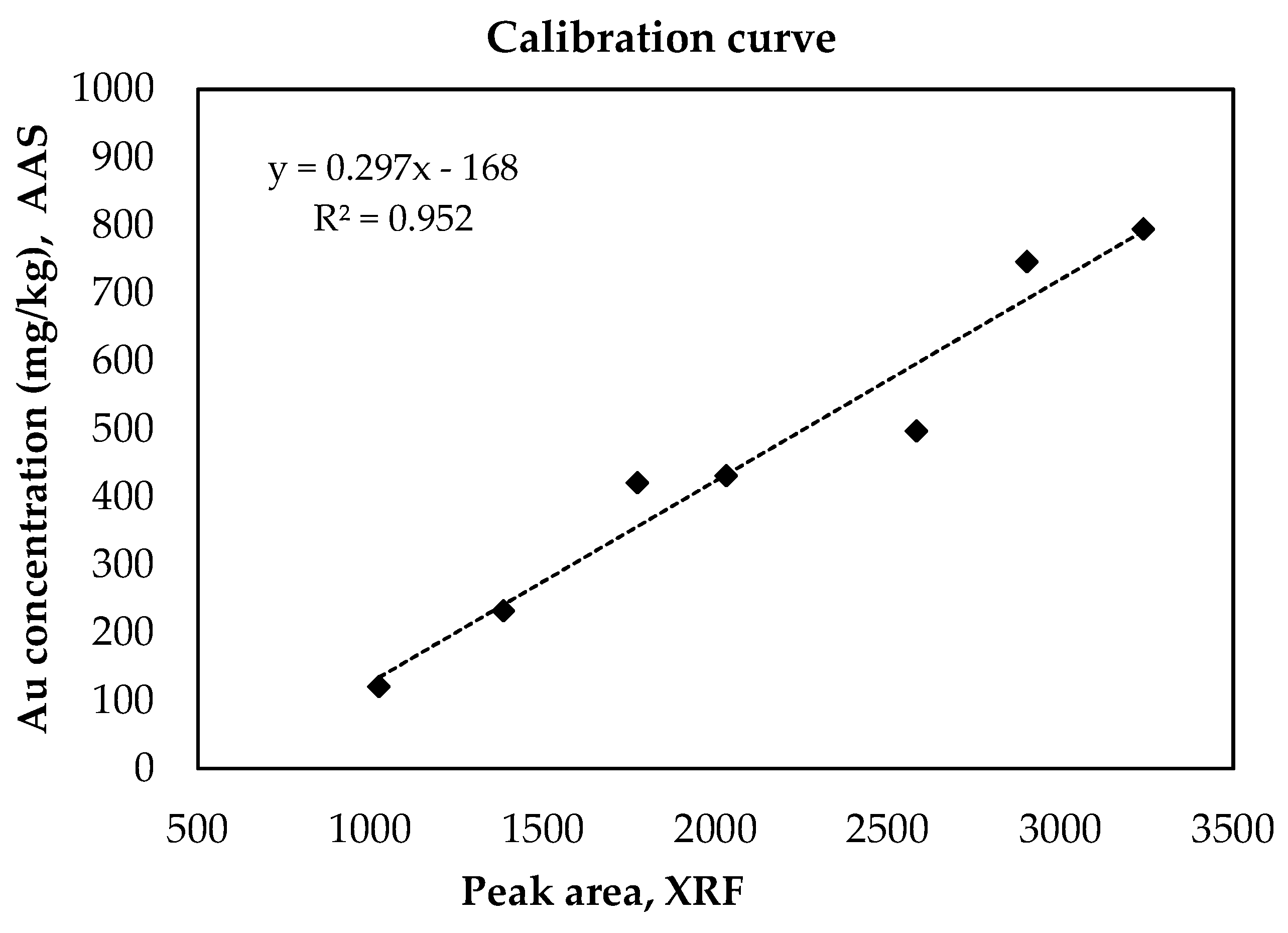
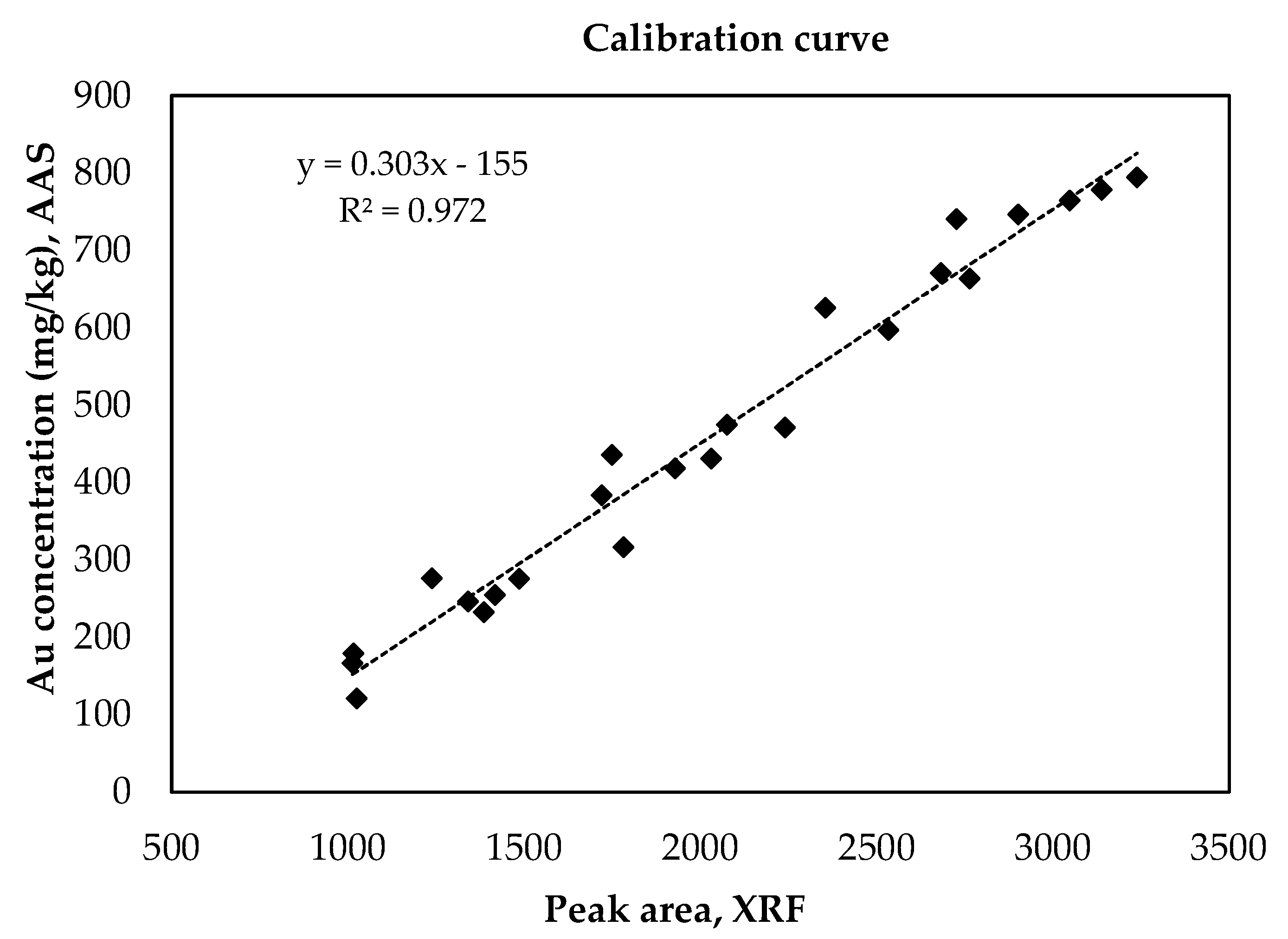
3.1. Calibration Curve Construction Using Real Matrices

Table 1 reports the peak areas and the gold concentrations determined by AAS for the 10 PCB samples analyzed for the construction of the calibration curve.
The gold concentration is within the range from 120.7 mg/kg to 1000.2 mg/kg, given the relatively high variability in gold concentration of the PCBs in waste mobiles; this waste is suitable for the construction of the gold calibration curve. For the concentration of gold greater than 800 mg/kg, the response of XRF in terms of peak area was not reliable, as it overly amplified the signal. For this reason, only seven out of ten standards were selected for the construction of curve calibration by excluding the concentration above 800 mg/kg (Figure 1).
The peak areas reported in Figure 1 were obtained by deconvolution of the spectra after the identification of all elements contained in the matrices. The deconvolution of the spectra was used to reduce interferences from other elements of the samples. The R2 is above 0.95. This curve was evaluated with other similar waste samples of PCBs to verify the robustness of the calibration and to calculate the deviation from the values determined by AAS.

3.2. Evaluation of the Calibration Curve

The first evaluation was performed by using 13 samples of PCB waste powders. Table 2 shows the gold concentration for AAS and XRF.
The average of the differences is ±28.4 mg/kg with a maximum value of 80.3 mg/kg (overestimation of XRF) and a minimum of −96.7 mg/kg (underestimation of XRF), considering the gold concentration obtained by AAS as a reference. The average RPD (%) on the 13 samples is 7.2%.
The samples used for the evaluation of the calibration curve were also used to improve it, as reported in Figure 2.
R2 has a higher value than that obtained by using seven PCB samples (see Figure 1).
In order to assess the existence of a correction factor to align the XRF results with those obtained by AAS and to consolidate the results, additional samples were used for the evaluation of the curve. More in detail, due to the lack of data in the ranges 250–400 mg/kg and 500–650 mg/kg, 10 samples obtained as mixtures of the previously standards were selected for the validation. The results are reported in Table 3.
From these data, it is possible to observe that for the samples 14 and 22, XRF provides unreliable values with an error higher than 150 mg/kg; to elaborate, XRF underestimates the values obtained by AAS. For the remaining eight samples, the difference between the values from the data provided by the two techniques was an average of 42 mg/kg; hence, an RPD of 17.3% was calculated. A trend seems to be emerging in relation to previous calculations: XRF underestimates the concentration of gold compared to AAS.
Once again, data used for the evaluation of the calibration curve added new standards to obtain a more reliable curve useful for gold measurement by FPXRF, as reported in Figure 3.
The curve was evaluated using new PCB samples with the aim of confirming the trend of XRF to underestimate the gold content. The results are reported in Table 4.
In this case, XRF overestimated the gold concentration obtained by AAS. The average difference for gold concentration measured by XRF and the quantitative value obtained with AAS for the same samples was ±72.6 mg/kg. Consequently, the error between the quantitative technique of atomic absorption spectroscopy and the technique of portable XRF observed for the 10 control samples resulted in a range of deviation of 13.4%, value significantly lower than 20% as established by EPA Method 6200 for portable fluorescence to consider acceptable the calibration [9]. The accuracy of the curve was estimated by RPD and, the obtained value was 14.7%, also confirms a good calibration curve [9].
In order to evaluate the goodness of the calibration curve, the gold concentration obtained by FPXRF and AAS was plotted, as shown in Figure 4.
The R2 of regression between the two sets of data is near 0.98, and the regression line matches the line well at a 45 degree, which is a sign of good accuracy of the curve.

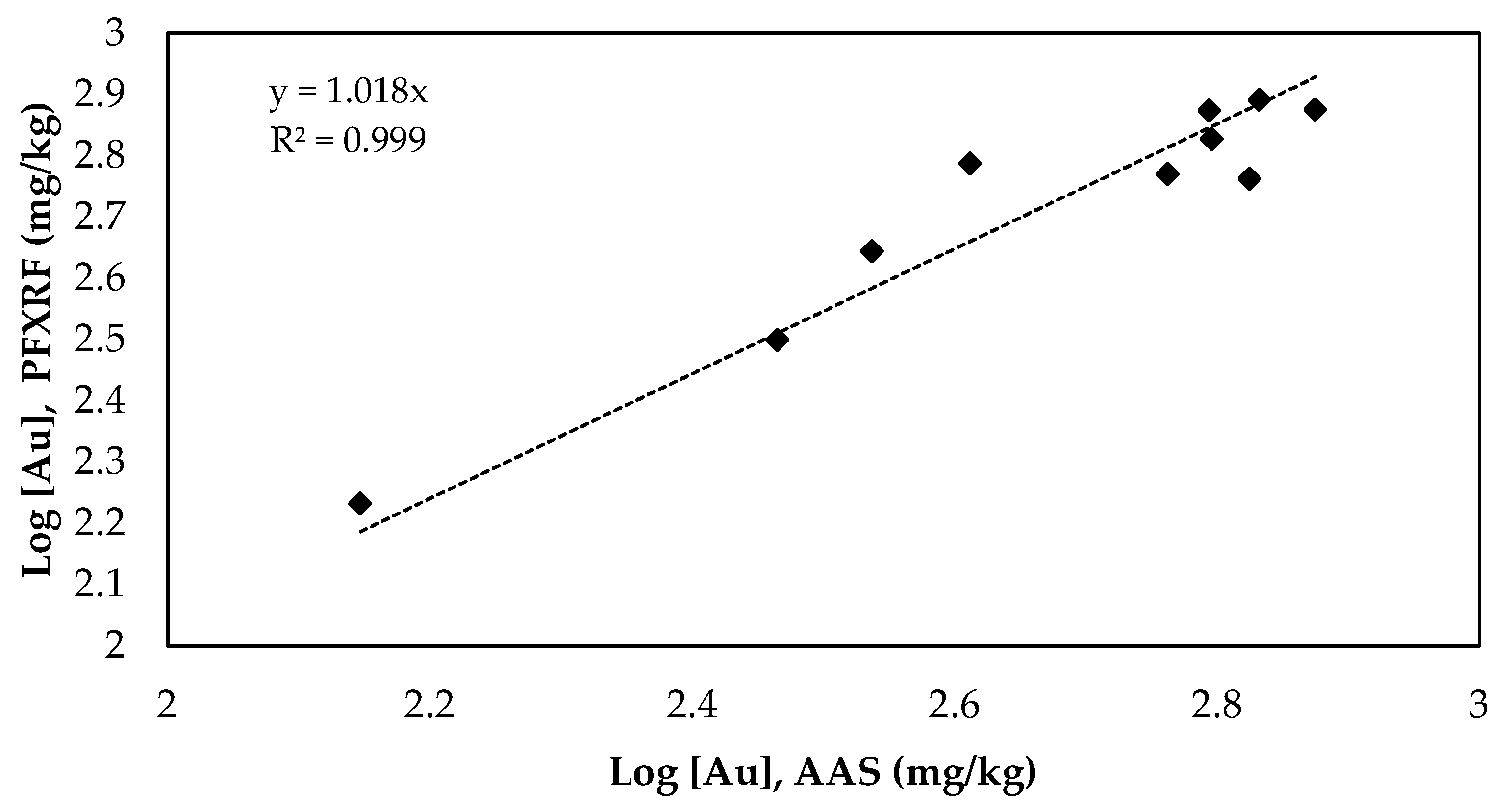
3.3. Statistical Analysis and FPXRF

The results of the Bland–Altman plot analysis are shown in Table 5 and Figure 5.
The mean gold concentration measured by FPXRF is 54.81 mg/kg lower than those measured by AAS. The accuracy of FPXRF for the gold measurement versus the AAS method is 80.19 mg/kg, and the limits of agreement (LA) are between −102.8 and 212.00 mg/kg. The range between the lower and the upper limit is 0.70 times the range between the minimum and maximum value measured with AAS.
The analysis showed that there are not outliers; in fact, all of the values are within the range of the lower and upper lines.
In regard to the regression analysis, two models were investigated for the estimation of the parameters. The first model is described by the following Equation (3):
Y = 0.8746X + 0.3861
R2 for this model is 0.920.
The second model consists of a line passing through the origin in the absence of the y-intercept. In this case, R2 is higher than that calculated with Equation (3) and equals 0.999. The value of the parameter is as follows:
Y = 1.018X
Equation (4) describes the data (Figure 6), and this was considered for validation.
The variance theorem was used to assess errors in the estimation of parameters: the value of the variance of error is σe2 = 0.005.
For the validation of the model, it was assumed that the measure of gold falls within the range defined by the chosen significance level (Equation (5)):
Yobserved = Ycalculated ± tα/2,n−1 σ*
where tα/2,n−1 is the t-Student value for a significance level of 95%, while σ* is the standard deviation of the predicted value (Y calculated) that depends on σe2, the number of samples, and the AAS values. The R2 value was 0.999; therefore, the model showed a linear relationship between the two measurement methods. R2 was used to classify the data obtained by FPXRF; according to EPA [11], in the specific case, the data qualitive level was assumed to be definitive (R2 > 0.900).
Table 6 and Figure 7 report the results of the statistical analysis.
The test of agreement revealed that the mean difference of measurements obtained with AAS and FPXRF is 72.6 mg/kg. This result is independent of gold concentration range, since the same mean difference was observed within the calibration range. The analysis of the obtained results is necessary considering that AAS data are affected by chemical attack procedures, analytical error of gold measurement, and spectral interferences due to the complexity of matrices [41]. R2 of linear regression (>0.90) analysis and RPD classification suggest that FPXRF analysis of gold concentrations in waste gives a quantitative measurement. Similar results were also obtained by other authors, as described in the work of Havukainen et al. [42].

4. Conclusions

Field-portable X-ray fluorescence spectrometers were used to determine the gold concentration from PCBs of waste mobile phones. The main aim was to determine whether this technique can replace conventional analytical techniques, such as atomic absorption spectrometry (AAS), that are more expensive and require more time consumption.
Firstly, a calibration curve was realized using waste samples of PCBs ground to a size below 0.5 mm and analyzed using FPXRFs at different acquisition times with five replications; then, the same samples were dissolved with aqua regia and analyzed using AAS to determine the quantitative gold content. The obtained results were associated with the FPXRFs response with the purpose of realizing a calibration curve (100–800 mg/kg Au). After validation of the curve, a statistical analysis was performed to determine the accuracy of the FPXRF measurements with respect to the AAS measurements. An RPD value of 14.7% was found, confirming a good calibration curve. Bolt–Altman analysis showed that the mean gold concentration measured by FPXRF is 54.81 mg/kg lower than those measured by AAS. The accuracy of the FPXRF gold measurement versus that of the AAS method is 80.19 mg/kg, and the limits of agreement are between −102.8 and 212.00 mg/kg. Moreover, the regression analysis shows a linear correlation between the FPXRF and AAS measurements.
FPXRF could be used for semi-quantitative analysis in waste treatment as a fast and non-consumable characterization of the samples in order to identify an economic prefeasibility of a possible recycling and recovery process or possible negotiations on waste management. A first screening of the material can be performed using XRF, which will showcase the advantages of this method of analysis, i.e., speed, portability, and the lower cost of measurements.

Author Contributions

Conceptualization, L.P. (Luigi Piga). and L.P. (Loris Pietrelli); formal analysis, N.M.I. and V.I.; investigation, N.M.I. and G.B.; resources, L.P. (Luigi Piga), F.M.; data curation, N.M.I., V.I.; writing–original draft preparation, N.M.I. and V.I.; supervision, L.P. (Luigi Piga)., L.P. (Loris Pietrelli) and F.M. All authors have read and agreed to the published version of the manuscript.

Funding

This research received no external funding.

Institutional Review Board Statement

Not applicable.

Informed Consent Statement

Not applicable.

Data Availability Statement

Not applicable.

Acknowledgments

The authors would like to thank Nike Srl for supplying the waste mobiles phones on which this work was carried out.

Conflicts of Interest

The authors declare no conflict of interest.

References

  1. Kilbride, C.; Poole, J.; Hutchings, T.R. A comparison of Cu, Pb, As, Cd, Zn, Fe, Ni and Mn determined by acid extraction/ICP-OES and ex situ field portable X-ray fluorescence analyses. Environ. Pollut. 2006, 143, 16–23. [Google Scholar] [CrossRef] [PubMed]
  2. Kalnicky, D.J.; Singhvi, R. Field portable XRF analysis of environmental samples. J. Hazard. Mater. 2001, 83, 93–122. [Google Scholar] [CrossRef] [Green Version]
  3. Hou, X.; He, Y.; Jones, B.T. Recent advances in portable X-ray fluorescence spectrometry. Appl. Spectrosc. Rev. 2004, 39, 1–25. [Google Scholar] [CrossRef]
  4. Drake, P.L.; Lawryk, N.J.; Ashley, K.; Sussell, A.L.; Hazelwood, K.J.; Song, R. Evaluation of two portable lead-monitoring methods at mining sites. J. Hazard. Mater. 2003, 102, 29–38. [Google Scholar] [CrossRef]
  5. Hall, G.E.M.; Bonham-Carter, G.F.; Buchar, A. Evaluation of portable X-ray fluorescence (pXRF) in exploration and mining. Geochem. Explor. Environ. Anal. 2014, 14, 99–123. [Google Scholar] [CrossRef] [Green Version]
  6. Simandl, G.J.; Stone, R.S.; Paradis, S.; Fajber, R.; Reid, H.M.; Grattan, K. An assessment of a handheld X-ray fluorescence instrument for use in exploration and development with an emphasis on REEs and related speciality metals. Miner. Deposita 2014, 49, 999–1012. [Google Scholar] [CrossRef]
  7. Young, K.E.; Evans, C.A.; Hodges, K.V.; Bleacher, J.E.; Graff, T.G. A review of the handheld X-ray fluorescence spectrometer as a tool for field geologic investigations on Earth and in a planetary surface exploration. Appl Geochem. 2016, 72, 77–87. [Google Scholar] [CrossRef] [Green Version]
  8. Ryan, J.G.; Shevais, J.W.; Li, Y.; Reagan, M.K.; Li, H.Y.; Heaton, D.; Godard, M.; Kirchenbaur, M.; Whattam, S.A.; Pearce, J.A.; et al. Application of a handheld X-ray fluorescence spectrometer for real-time, high-density quantitative analysis of drilled igneous rocks and sediments during IODP Expedition 352. Chem. Geol. 2017, 451, 55–56. [Google Scholar] [CrossRef] [Green Version]
  9. US EPA. Field Portable X-Ray Fluorescence Spectrometry for the Determination of Elemental Concentrations in Soil and Sediment; Method 6200; US EPA: Washington, DC, USA, 1998. [Google Scholar]
  10. US EPA. Innovative Technology Verification Report: XRF Technologies for Measuring Trace Elements in Soil and Sediment; Office of Research and Development; US EPA: Washington, DC, USA, 2006. [Google Scholar]
  11. US EPA. Field Portable X-ray Fluorescence Spectrometry for the Determination of Elemental Concentrations in Soil and Sediment; SW-846 Test Method 6200; US EPA: Washington, DC, USA, 2007. [Google Scholar]
  12. Radu, T.; Diamond, D. Comparison of soil pollution concentrations determined using AAS and portable XRF techniques. J. Hazard. Mater. 2009, 171, 1168–1171. [Google Scholar] [CrossRef]
  13. Parsons, C.; Grabulosa, E.M.; Pili, E.; Floor, G.H.; Roman-Ross, G.; Charlet, L. Quantification of trace arsenic in soils by field-portable X-ray fluorescence spectrometry: Considerations for sample preparation and measurement conditions. J. Hazard. Mater. 2013, 262, 1213–1222. [Google Scholar] [CrossRef]
  14. Mejía-Piña, G.; Huerta-Diaz, M.A.; González-Yajimovich, O. Calibration of handheld X-ray fluorescence (XRF) equipment for optimum determination of elemental concentrations in sediment samples. Talanta 2016, 161, 359–367. [Google Scholar] [CrossRef]
  15. Brent, R.N.; Wines, H.; Luther, J.; Irving, N.; Collins, J.; Drake, B.L. Validation of handheld X-ray fluorescence for in situ measurement of mercury in soils. J. Environ. Chem. Eng. 2017, 5, 768–776. [Google Scholar] [CrossRef]
  16. Marguì, E.; Queralt, I.; Hidalgo, M. Application of X-ray fluorescence spectrometry to determination and quantitation of metals in vegetal material. Trac. Trend. Anal. Chem. 2009, 28, 362–372. [Google Scholar] [CrossRef]
  17. Chou, J.; Clement, G.; Bursavich, B.; Elbers, D.; Cao, B.; Zhou, W. Rapid detection of toxic metals in non-crushed oyster shells by portable X-ray fluorescence spectrometry. Environ. Pollut. 2010, 158, 2230–2234. [Google Scholar] [CrossRef]
  18. Weindorf, D.C.; Zhu, Y.; Chakraborty, S.; Bakr, N.; Huang, B. Use of portable X-ray fluorescence spectrometry for environmental quality assessment of peri-urban agriculture. Environ. Monit. Assess. 2012, 184, 217–227. [Google Scholar] [CrossRef] [PubMed]
  19. Turner, A.; Solman, K.R. Analysis of the elemental composition of marine litter by field-portable-XRF. Talanta 2016, 159, 262–271. [Google Scholar] [CrossRef] [PubMed] [Green Version]
  20. Bull, A.; Brown, M.T.; Turner, A. Novel use of field-portable-XRF for the direct analysis of trace elements in marine macroalgae. Environ. Pollut. 2017, 200, 228–233. [Google Scholar] [CrossRef] [PubMed]
  21. Turner, A. In situ elemental characterization of marine micro-plastics by portable XRF. Mar. Pollut. Bull. 2017, 124, 286–291. [Google Scholar] [CrossRef] [PubMed]
  22. Turner, A.; Filella, M. Field-portable-XRF reveals the ubiquity of antimony in plastic consumer products. Sci. Total Environ. 2017, 584–584, 982–989. [Google Scholar] [CrossRef] [PubMed] [Green Version]
  23. Higueras, P.; Oyarzun, R.; Iraizoz, J.M.; Lorenzo, S.; Esbrí, J.M.; Martínez-Coronado, A. Low-cost geochemical surveys for environmental studies in developing countries: Testing a field portable XRF instrument under quasi-realistic conditions. J. Geochem. Explor. 2012, 113, 3–12. [Google Scholar] [CrossRef] [Green Version]
  24. Rowe, H.; Hughes, N.; Robinson, K. The quantification and application of handheld energy-dispersive x-ray fluorescence (ED-XRF) in mudrock chemostratigraphy and geochemistry. Chem. Geol. 2012, 324–325, 122–131. [Google Scholar] [CrossRef]
  25. Cohen, D.R.; Cohen, E.J.; Graham, I.T.; Soares, G.G.; Hand, S.J.; Archer, M. Geochemical exploration for vertebrate fossils using field portable XRF. J. Geochem. Explor. 2017, 181, 1–9. [Google Scholar] [CrossRef]
  26. Figi, R.; Nagel, O.; Tuchschmid, M.; Lienemanna, P.; Gfeller, U.; Bukowiecki, N. Quantitative analysis of heavy metals in automotive brake linings: A comparison between wet-chemistry based analysis and in-situ screening with a handheld X-ray fluorescence spectrometer. Anal. Chim. Acta 2010, 676, 46–52. [Google Scholar] [CrossRef] [PubMed]
  27. Kloos, D. Underkarat jewelry: The perfect crime? Investigations and analysis of jewelry using XRF. ICCD Adv. X-Ray Anal. 2003, 46. [Google Scholar]
  28. Su, Q.; Yin, Y. ED-XRF determination on the content of cadmium and lead in polymeric materials. Chem. Res. Appl. 2015.
  29. Adami, K.Z. Variational Methods in Bayesian Deconvolution; PHYSTAT2003; SLAC: Stanford, CA, USA, 8–11 September 2003. [Google Scholar]
  30. Curis, E.; Osan, J.; Falkenberg, G.; Benazeth, S.; Torok, S. Simulating systematic errors in X-ray absorption spectroscopy experiments: Sample and beam effects, Spectrochim. Acta Part. B 2005, 60, 841–849. [Google Scholar] [CrossRef]
  31. Elam, W.T.; Scruggs, B.; Eggert, F.; Nicolosi, J.A. F-13 Advantages and Disadvantages of Bayesian Methods for Obtaining XRF Net Intensities. Powder Diffr. 2010, 25, 215. [Google Scholar] [CrossRef] [Green Version]
  32. Manninen, S.; Pitkanen, T.; Koikkalainen, S.; Pakkari, T. Study of the ratio of elastic to 333 inelastic scattering of photons. Int. J. Appl. Radiat. Isot. 1984, 35, 93–98. [Google Scholar] [CrossRef]
  33. Sherman, J. The theoretical derivation of fluorescent X-ray intensities from mixtures. Spectrochim. Acta. 1955, 7, 283–306. [Google Scholar] [CrossRef]
  34. Rousseau, R.M.; Boivin, J.A. The Fundamental Algorithm: A natural extension of the Sherman equation, part I: Theory. Rigaku J. 1998, 15, 13–15. [Google Scholar]
  35. Rousseau, R.M. The quest for a Fundamental Algorithm in X-ray fluorescence analysis and calibration. Open Spectrosc, J. 2009, 3, 31–42. [Google Scholar] [CrossRef] [Green Version]
  36. Criss, J.W.; Birks, L.S. Calculation methods for fluorescent Xray spectrometry, empirical coefficients vs. fundamental parameters. Anal. Chem. 1968, 40, 1080–1087. [Google Scholar] [CrossRef]
  37. Conrey, R.M.; Goodman-Elgar, M.; Bettencourt, N.; Seyfarth, A.; Van Hoose, A.; Wolff, J.A. Calibration of a portable X-ray fluorescence spectrometer in the analysis of archaeological samples using influence coefficients. Geochem. Explor. Environ. A 2014, 14, 291–301. [Google Scholar] [CrossRef]
  38. Ravansari, R.; Wilson, S.C.; Tighe, M. Portable X-ray fluorescence for enviromental assessment of soils: Not just a point and shoot method. Environ. Int. 2020, 134, 105250. [Google Scholar] [CrossRef] [PubMed]
  39. Imanishi, Y.; Bando, A.; Komatani, S.; Wada, S.; Tsuji, K. Experimental parameters for XRF analysis of soils. Adv. X-ray Anal. 2010, 53, 248–255. [Google Scholar]
  40. Ranganathan, P.; Pramesh, C.S.; Aggarwal, R. Common pitfalls in statistical analysis: Measure of agreement. Perspect. Clin. Res. 2017, 8, 187–191. [Google Scholar] [CrossRef] [PubMed]
  41. US EPA. Flame Atomic Absorption Spectrophotometry; Method 7000B; US EPA: Washington, DC, USA, 2007. [Google Scholar]
  42. Havukainen, J.; Hiltunen, J.; Puro, L.; Horttanainen, M. Applicability of a field portable X-ray fluorescence for analyzing elemental concentration of waste samples. Waste Manag. 2019, 83, 6–13. [Google Scholar] [CrossRef]
Figure 1. Calibration curve for FPXRF obtained by using real samples of PCBS as standards (number of standards: 7).
Processes 09 01618 g001
Figure 2. Calibration curve for FPXRF obtained by using real samples of PCBS as standards (number of standards: 16).
Processes 09 01618 g002
Figure 3. Calibration curve for FPXRF obtained by using real samples of PCBS as standards (number of standards: 24).
Processes 09 01618 g003
Figure 4. Regression of FPXRF and AAS concentration.
Processes 09 01618 g004
Figure 5. Bland–Altman analysis of agreement between Au measurement using XRF and AAS (mg/kg).
Processes 09 01618 g005
Figure 6. Regression of FPXRF data and AAS analysis.
Processes 09 01618 g006
Figure 7. Statistical confidence determined for the model (4).
Processes 09 01618 g007
Table 1. Peak area for the XRF analysis and the relative concentration of gold obtained by AAS.
PCB SamplesAu Peak Area—XRF AnalysisAu Concentration (mg/kg)—AAS Analysis
S11385.0232.5
S29451.4999.8
S32901.4746.6
S42581.8497.0
S51024.6120.7
S63238.8794.5
S71772.4420.7
S820,146.0943.1
S930,044.61000.2
S102030.4431.2
Table 2. Analysis of PCB samples: gold determination by XRF using the calibration curve and by AAS.
SampleAu Concentration—AAS
(mg/kg)
Au Concentration—XRF
(mg/kg)
Difference
(mg/kg)
RPD
(%)
1471.0495.124.15.0
2430.6510.980.317.1
3451.2453.01.80.4
4625.9529.2−96.716.7
5254.4251.0−3.41.3
6418.5402.6−15.93.9
7764.3745.7−18.62.5
8166.5133.8−32.721.8
9778.1796.518.42.3
10663.5650.3−13.22.0
11474.5477.93.40.7
12316.3359.042.712.6
13246.0228.4−17.67.4
average ±28.47.2
Table 3. Analysis of PCB samples: gold determination by XRF using the calibration curve and by AAS.
SampleAu Concentration—AAS (mg/kg)Au Concentration—XRF (mg/kg)Difference
(mg/kg)
RPD
(%)
14650.4487.5−162.928.6
15597.4601.03.60.6
16275.6278.12.50.9
17383.8350.2−33.69.2
18671.0646.9−24.13.7
19179.0133.2−45.829.3
20276.2201.8−74.431.1
21435.6359.3−76.319.2
22566.5380.5−186.039.3
23740.3660.8−79.511.3
average ± 68.917.3
Table 4. Analysis of PCB samples: gold determination by XRF using the calibration curve and by AAS.
SampleAu Concentration—AAS (mg/kg)Au Concentration—XRF (mg/kg)Difference
(mg/kg)
RPD
(%)
24578.8588.49.61.6
25668.4579.5−88.914.2
26625.7672.546.87.2
27291.8316.324.58.1
28680.0779.099.013.6
29409.3612.7203.439.8
30750.2751.51.30.2
31140.3170.730.419.3
32622.5747.7125.218.3
33344.5441.396.824.6
average ± 72.614.7
Table 5. Results of Bland–Altman analysis of agreement between Au measurement using XRF and AAS (mg/kg).
Bland–Altman Analysis (mg/kg)
Mean of difference54.81
SD of difference80.19
Limits of agreement
Lower−102.38
Upper212.00
Table 6. Statistical results of the Au concentration.
Au Concentration Range (mg/kg)
AAS
Au Concentration Range (mg/kg)
FPXRF
R2Gradient of LineY-InterceptVarianceStandard DeviationConfidential IntervalData
Quality Level
140.3–750.2170.7–7790.9991.018--0.0110.104Range 0.061–0.154
Average 0.080
Definitive
Publisher’s Note: MDPI stays neutral with regard to jurisdictional claims in published maps and institutional affiliations.

