Research on Regional Short-Term Power Load Forecasting Model and Case Analysis

Abstract

Integrated energy services will have multiple values and far-reaching significance in promoting energy transformation and serving “carbon peak and carbon neutralization”. In order to balance the supply and demand of power system in integrated energy, it is necessary to establish a scientific model for power load forecasting. Different algorithms for short-term electric load forecasting considering meteorological factors are presented in this paper. The correlation between electric load and meteorological factors is first analyzed. After the principal component analysis (PCA) of meteorological factors and autocorrelation analysis of the electric load, the daily load forecasting model is established by optimal support vector machine (OPT-SVM), Elman neural network (ENN), as well as their combinations through linear weighted average, geometric weighted average, and harmonic weighted average method, respectively. Based on the actual data of an industrial park of Nantong in China, the prediction performance in the four seasons with the different models is evaluated. The main contribution of this paper is to compare the effectiveness of different models for short-term electric load forecasting and to give a guideline to build the proper methods for load forecasting.

1. Introduction

Integrated energy services will have multiple values and far-reaching significance in promoting energy transformation and serving “carbon peak and carbon neutralization”. Before the implementation of integrated energy services, in order to balance the supply and demand of the power system, it is necessary to establish a scientific model for power load forecasting. The balance of supply and demand in the power system plays an important role in regional economic and social development. To improve the quality of power supply, it is important to analyze various characteristics of regional electric load and establish a proper model for the short-term electrical load forecasting [1].

Many factors affect electric load forecasting, including social-economic factors, such as population and industrial structure, and meteorological conditions [2,3]. Therein, complex and changeable meteorological factors are essential factors in load forecasting and have the greatest impact on forecast results [2]. Forecasting that considers meteorological factors can improve forecasting accuracy.

According to relevant statistics, in large cities with large population, residential power consumption in summer can reach 50% or even higher of the total power load. The prediction of residential power load plays an important role in regional energy allocation, energy-saving control, and power grid reliability. At the same time, residential power load shows the characteristics of complexity and uncertainty, which is closely related to temperature, humidity, wind speed, week type, building function, building area, industrial structure, and other factors.

In short-term load forecasting, the processing methods of meteorological factors mainly include the following ideas: (1) Do not consider the influence of meteorological factors; (2) Only the influence of single meteorological factor shall be considered; (3) Considering the influence of multiple meteorological factors without coupling effect; (4) Considering the influence of meteorological index formed by coupling multiple meteorological factors; (5) Consider the influence of real-time meteorological factors. In the actual prediction process, the appropriate treatment scheme is selected according to local conditions in combination with the actual local weather and load conditions.

Load forecasting can be divided into ultra-short-term, short-term, medium-term, and long-term according to different purposes. Short-term load forecasting refers to daily load forecasting and weekly load forecasting. It is necessary to fully study the law of power grid load changes and analyze the relevant factors of load changes for arrangement of daily scheduling plan or weekly scheduling plan.

Extensive research has been done on load forecasting, and the algorithms can be divided into two groups. Traditional statistical algorithms including the time series model [4,5,6] and the linear regression model [7] are the early and widely developed methods for load forecasting. It is modeled only based on load time series, which is computationally fast. However, short-term load forecasting is affected by many factors as mentioned above. When the weather changes greatly or the holidays occur, these models fail to forecast accurately [8]. Therefore, the second load forecasting algorithm that considers meteorological factors came into being. It takes into account weather and calendar factors to make the forecast results closer to the actual situation. These modern intelligent algorithms include the artificial neural network (ANN) [9,10,11], the expert system [12], support vector machine(SVM) [13,14,15,16], etc. Though these individual forecasting models obtain satisfactory performance, each model has unavoidable drawbacks, and their performance varies under different conditions, which results in risks and limitations in the practical applications [17].

Thus, it is possible to consider combining different individual forecasting models. In 1969, Bates and Granger made a systematic study on the combination forecasting method for the first time and then aroused great interest in combination forecasting models [18]. According to the pros and cons of individual algorithms, the combination of these algorithms can reduce the risks of the individual method and achieve better forecasting performance. Various combinations are proposed, such as the BP neural network model combined with the gray theory model based on variable weights [19], different types of neural network combinations based on non-positive constraint theory [20], SVM combined with chaos theory [21], etc. These researches of combination models mainly focus on the determination of the optimal weights to improve the forecast accuracy, and, meanwhile, avoid falling into local optimal solution, lower convergent rate, and increasing modeling complexity [22,23,24].

In addition, some recent papers have also proposed some short-term load forecasting methods: a novel hybrid forecasting algorithm is proposed in [25]. The proposed hybrid forecasting method is based on locally weighted support vector regression (LWSVR) and the modified grasshopper optimization algorithm (MGOA). Obtaining the appropriate values of LWSVR parameters is vital to achieving satisfactory forecasting accuracy. Therefore, the MGOA is proposed in this paper to optimally select the LWSVR’s parameters. The proposed MGOA can be derived by presenting two modifications on the conventional GOA in which the chaotic initialization and the sigmoid decreasing criterion are employed to treat the drawbacks of the conventional GOA. There are also other related papers, e.g., the work in [26] proposes an ultra-short-term power load forecasting method based on two-layer xgboost (extreme gradient boosting) algorithm. The work in [27] proposes a short-term power load forecasting model based on similar day selection and multi-integration combination. In [28], particle swarm optimization (PSO) is proposed to optimize the neural network model of quantum weighted gated circulating unit to predict short-term power load. The work in [29] introduces K-means clustering analysis technology based on cosine similarity to predict short-term power load. The work in [30] proposes a load forecasting method based on improved deep belief network algorithm.

It can be seen that there are many short-term load forecasting methods, such as time series model, multiple linear regression, support vector machine, and so on. Compared with other traditional algorithms, support vector machine has better prediction effect for small samples and has the advantages of strong learning ability and high precision in processing high-dimensional data. However, the prediction effect of support vector machine is closely related to the quality of parameter estimation. At present, the commonly used grid parameter optimization methods have a large amount of calculation and limited parameter estimation accuracy. Using an intelligent optimization algorithm to find the global optimal parameter combination has gradually become an effective way to improve the application effect of support vector machine. In light of this, by coupling a simulated annealing particle swarm optimization algorithm and support vector machine, an optimized support vector machine model is constructed to study the short-term load forecasting effect under different meteorological variable input conditions and analyze the influence of meteorological factors on load forecasting.

In the field of power load forecasting, static neural network, mainly represented by BP neural network, is most widely used. This kind of model actually transforms dynamic time modeling into static space modeling, resulting in its insufficient ability to capture the highly complex time-varying characteristics of load. Therefore, Elman neural network with dynamic adaptive time-varying characteristics is applied after adding a receiving layer on BP neural network.

For the short-term load forecasting of regional power system, the problems existing in the current research include the following.

• In the practical application of power load forecasting models, most models and methods cannot predict the load according to different regions and different utilization types, and there is a lack of intelligent forecasting methods that can effectively adapt to a variety of conditions and improve the accuracy.
• The current research lacks in-depth analysis of regional basic situation, economy, population and industrial structure, analysis of regional power load characteristics, understanding of environmental and meteorological factors, and detailed analysis of the impact of environmental and meteorological factors on load forecasting.
• In the actual dispatching of power system, seasonal power shortage occurs from time to time, especially in summer and winter. Therefore, it is necessary to strengthen the research on seasonal power load forecasting in order to meet the power supply demand more reasonably.

This paper presents some combined models for short-term load forecasting. It integrates simulated annealing OPT-SVM and ENN through time-varying weights selection. Compared with other traditional algorithms, support vector machines have better prediction effects for small samples. The advantages of strong learning ability and high accuracy when processing high-dimensional data are also very prominent. The Elman neural network has better generalization and prediction ability for nonlinear and high-frequency time series data. The proposed models can take into account regional power load characteristics and their correlation with meteorological factors such as temperature, humidity, wind speed, and sunshine. On the one hand, they can improve the adaptability of the power dispatching department to regional power load changes; on the other hand, they can improve the accuracy of load forecasting to meet the demand of regional power load. The accuracy of short-term electrical load forecasting based on single OPT-SVM and ENN varies in different periods. The weighted combination of the results of different forecasting models in each period could result in higher accuracy of load forecasting. To this end, the time history of the contribution of each single model to the combined forecasting is studied. The effectiveness of the combination forecasting model is analyzed from the statistical accuracy so as to provide a useful reference for deepening the application of the time-varying weight combination model in short-term load forecasting.

The innovation of our paper is to find out a time-varying weight combination model which takes the results of two single models of OPT-SVM and Elman NN as input, studies the time history changes of each single model’s contribution to the combined forecasting, and uses statistics methods to analyze the effectiveness of the combined model, providing a useful reference for deepening the application of time-varying weight combination models in short-term load forecasting.

The rest of this paper is organized as follows. The experimental data are described in Section 2. In Section 3, the mathematical principles and processes of the proposed models are described in detail. Furthermore, Section 4 presents and discusses the forecasting results. Finally, the proposed models are summarized in Section 5.

2. Data Preparation

Under the influence of meteorological and other factors, regional power load often presents complex time-varying characteristics of continuity, nonlinearity, and multifrequency nesting. Therefore, in order to establish a scientific and accurate power load forecasting model, it is necessary to understand the time-varying characteristics of regional power load, analyze the correlation between power load and meteorological factors, and provide a priori knowledge for selecting the key influencing factors of power load forecasting.

The basic data of this paper come from the actual load demand data of an industrial park in Nantong, Jiangsu, China from 1 March 2016 to 28 February 2017. These data contain the following.

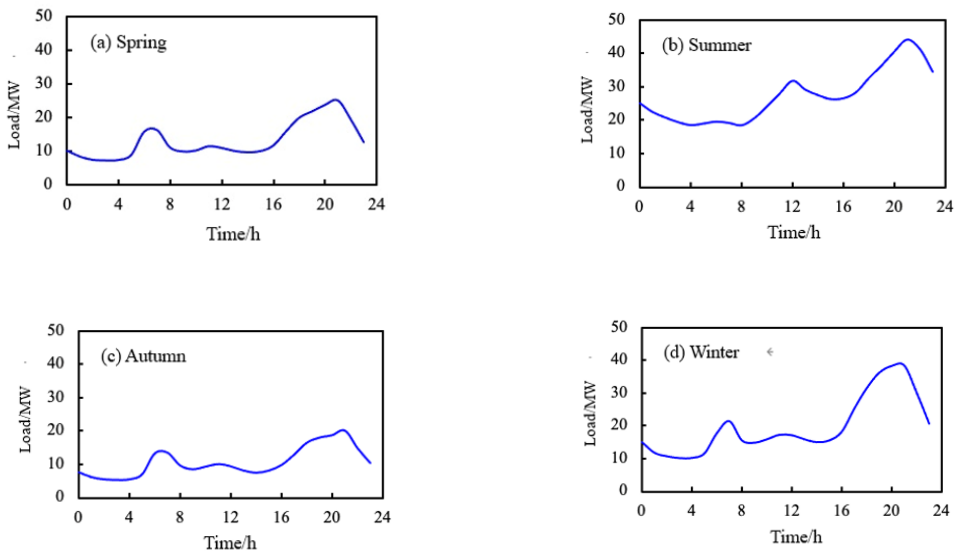
• Load demand data with a time interval of 15 min for industries, residents, and businesses; then, the hourly load demand and daily load demand are derived by accumulation, and the daily load curve is given in Figure 1;
• Meteorological data (e.g., temperature, relative humidity, wind speed, evaporation, and surface temperature) of every hour from Nantong Weather Station.

The studied industrial park area is about 170 km², with relatively concentrated distribution, simple terrain, and less-fluctuated climate, so one weather station can effectively cover the area.

The first three-quarters of the remaining load sequence length after excluding the pre-ordered autocorrelation load is used as the training sample, and the last one-quarter as the prediction verification sample; the modeling period and forecasting period are determined according to the four seasons and the load autocorrelation time lag as follows:

• Spring: March 5 to May 11 as modeling period, totaling 68 days, and May 11 to June 3 as forecasting period, totaling 23 days;
• Summer: June 11 to August 12 as modeling period, totaling 63 days, and August 13 to September 3 as forecasting period, totaling 22 days;
• Autumn: September 12 to November 11 as modeling period, totaling 63 days, and November 12 to December 3 as forecasting period, totaling 21 days;
• Winter: December 6 to February 6 (2017) as modeling period, totaling 63 days, and February 7 to February 28 as forecasting period, totaling 21 days.

During the preprocessing of the raw data, horizontal and vertical processing methods are used here to deal with abnormal data [31], and the Least squares method is applied for curve fitting to obtain the missing data. The power load forecasting model established should consider the influence of meteorological factors, and the meteorological factors, such as temperature, humidity, precipitation, sunshine days, wind speed, and electricity load, have different dimensions and units and cannot be used directly. Therefore, it is necessary to standardize all relevant factors so that all data are in the same order of magnitude.

Furthermore, the different types of meteorological data are normalized as follows:

$$Y=\frac{I_i-I_{min}}{I_{max}-I_{min}}$$

(1)

where Y is the normalized data, and $I_i$, $I_{min}$, and $I_{max}$ are the current sample value, minimum, and maximum of the training data, respectively.

3. Optimal Combined Model Considering Meteorological Factors

This paper improves the results of short-term load forecasting by the steps as shown in Figure 2.

3.1. Data Optimization

The pre-ordered autocorrelation load and comprehensive meteorological factors are taken as the input of the forecasting model. Therefore, the processing of the data is introduced as follows.

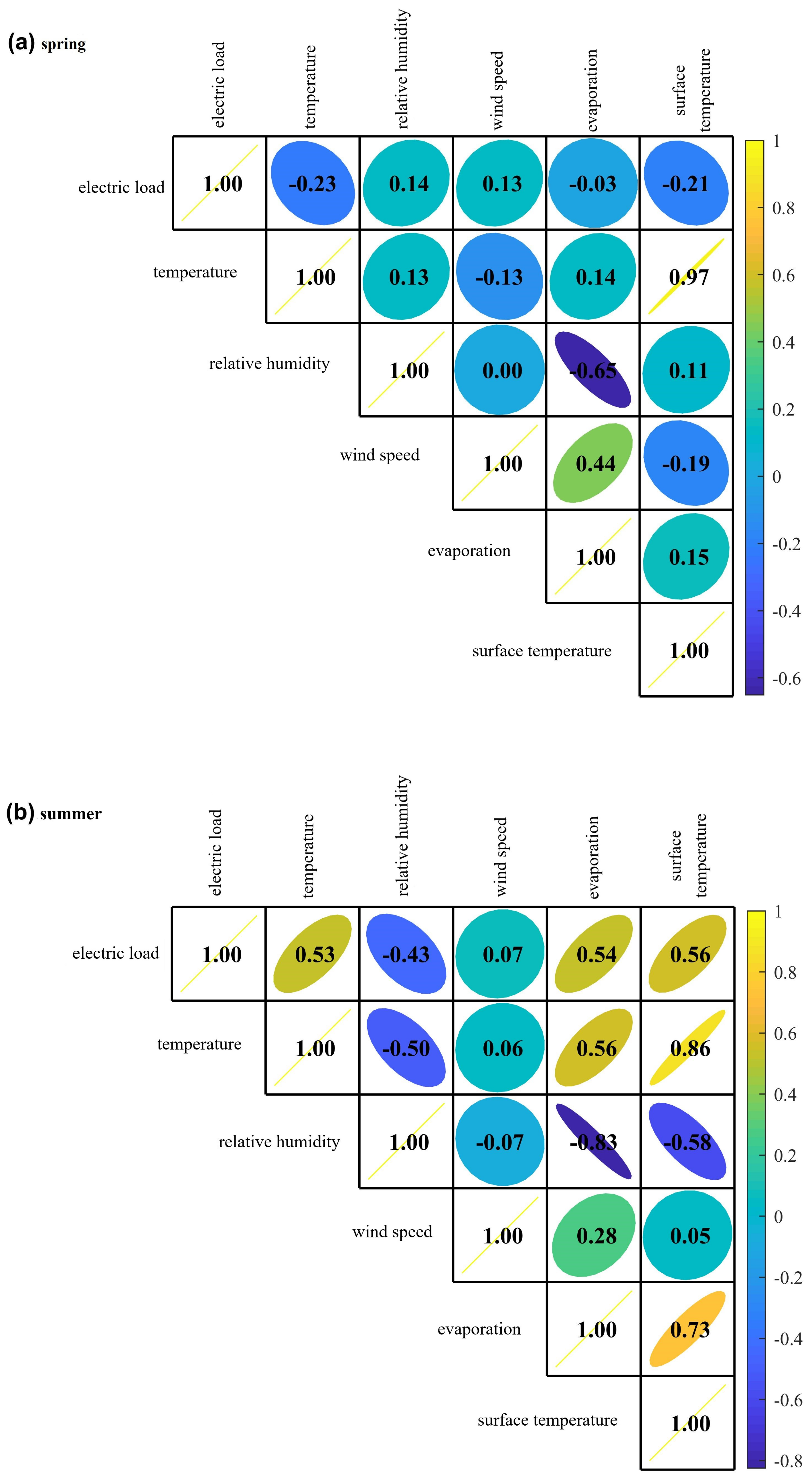
3.1.1. Correlation Analysis

First of all, the correlation analysis between electric load and meteorological factors is necessary. Pearson correlation coefficient is a measure of linear correlation between two sets of data, which has a value between −1 and 1. It is defined as

$${\rho }_{X,Y}=\frac{cov\left(X,Y\right)}{{\sigma }_X{\sigma }_Y}=\frac{E\left[\left(X-{\mu }_X\right)\left(Y-{\mu }_Y\right)\right]}{{\sigma }_X{\sigma }_Y}$$

(2)

where ${\rho }_{X,Y}$ represents the overall correlation coefficient, X and Y are two variables, $cov(X,Y)$ is the covariance of the variables X and Y, ${\mu }_X$ and ${\mu }_Y$ are the expectations of the variables X and Y, and ${\sigma }_X$ and ${\sigma }_Y$ are the standard deviations of the variables X, Y.

3.1.2. Principal Component Analysis (PCA)

There could exist correlations between different meteorological factors so that multiple meteorological variables may contain redundant information. PCA can be used to extract main feature factors from multiple meteorological factors for dimensionality reduction. It replaces the original variables with fewer new variables and enables these new variables to retain the original full variable information as much as possible. The detailed steps of PCA can be found in [32].

3.1.3. Autocorrelation Analysis of Electrical Load

The pre-ordered autocorrelation load is taken as the input of the proposed load forecasting model in this paper, and the autocorrelation time lag needs to be determined. The pre-ordered autocorrelation load time lag is determined according to the autocorrelation function (ACF) in [33].

3.2. Model Description

The proposed combined model integrates two individual models (i.e., OPT-SVM and ENN) based on the time-varying optimal weight selection. OPT-SVM and ENN both have good forecasting performance.

3.2.1. Optimal Supporting Vector Machine (OPT-SVM)

The basic idea of SVM algorithm is to construct an optimal hyperplane from the sample space or feature space to make the margin between different types of data points as far as possible. Given the sample sets $\left\{x_i,y_i\right\},i=1,2,\dots ,n$, $x_i$ is the input sample, $y_i$ is the output sample, and n is the total number of samples. The nonlinear load forecasting SVM model is expressed as

$$f\left(x\right)={\omega }^T\phi \left(x\right)+b$$

(3)

where $\phi \left(x\right)$ denotes the nonlinear mapping from the input space to high-dimensional feature space. $\omega$ is the weight vector and b is constant. They can be obtained by the principle of structural minimization, and the optimization target can be expressed as follows:

$$\frac{1}{2}{\omega }^2+c\underset{i=1}{\sum ^n}{\left|y_i-\left(\omega ,\phi \left(x_i\right)\right)-b\right|}_{\epsilon }$$

(4)

with c as penalty factor.

Introducing slack variables ${\xi }_i$ and ${\xi }_i^{*}$ into (4), it turns into

$$\frac{1}{2}{∥\omega ∥}^2+c\underset{i=1}{\sum ^n}\left({\xi }_i+{{\xi }_i}^{*}\right),\mathrm{s}.\mathrm{t}.\left\{\begin{array}{c}{y}_i-\left({\omega }^T\left(x_i\right)+b\right)\le \epsilon +{{\xi }_i}^{*}\\ \left({\omega }^T\phi \left(x_i+\mathrm{b}\right)\right)-y_i\le \epsilon +{\xi }_i\\ {\xi }_i,{{\xi }_i}^{*}\ge 0,i=1,\dots ,n\end{array}\right.$$

(5)

By introducing Lagrange multiplier $\alpha$, we transform Equation (5) into

$$f\left(x,a\right)=\underset{i=1}{\sum ^n}\left({{\alpha }_i}^{*}-{\alpha }_i\right)K\left(x_i,x\right)+b$$

(6)

where $K(x,x_i)$ is the kernel function. Here, we choose Gauss radial basis function (GRBF) as kernel function for its good analytical performance. GRBF is expressed as

$$K\left(x_i,x_j\right)=e^{-\gamma {∥x_i-x_j∥}^2}$$

(7)

where $\gamma$ is a tunable parameter.

Error penalty parameter c and kernel function parameter $\gamma$ are the two key parameters to the SVM. Compared with other traditional algorithms, support vector machines have better prediction effects for small samples. The advantages of strong learning ability and high accuracy when processing high-dimensional data are also very prominent. However, the prediction effect of support vector machines is closely related to the quality of parameter estimation. Currently, the commonly used gridding parameter optimization method has a large amount of calculation and limited parameter estimation accuracy. The use of intelligent optimization algorithms to find the global optimal parameter combination has gradually become an improved support vector and the most effective way to attain the machine application effect. Particle Swarm Optimization (PSO), as an excellent representative algorithm with clear principles and simple calculations, has been widely used in solving optimization problems. PSO is a swarm intelligence evolutionary computation technology based on iterative optimization. Furthermore, the simulated annealing algorithm is introduced to the PSO algorithm to increase its global optimization ability. The specific steps of the algorithm can refer to the work in [34]. Here, we utilize PSO to solve the optimal SVM parameters to avoid lengthy calculations. Because of this, this chapter builds an optimized support vector machine model by coupling the simulated annealing particle swarm optimization algorithm and support vector machine to study the effect of short-term load forecasting under different meteorological variable input conditions and analyze the influence of meteorological factors on load forecasting.

According to the description of simulated annealing PSO and SVM above, the algorithm of OPT-SVM for electric load forecasting proceeds as follows:

• Take the first three-quarters of the load sequence as the training sample, and the last one-quarter as the prediction verification sample. Determine the modeling period and forecast period in terms of the division of seasons and autocorrelation load time lag.
• Initialize the parameters of simulated annealing PSO algorithm, including number of particles L, particle dimension D, learning factors $c_1$, $c_2$, initial temperature $T_0$, cooling rate ${\alpha }_c$, and maximum number of iterations M.
• Taking the maximum certainty coefficient of SVM as the objective function, use the simulated annealing PSO algorithm to optimize the penalty factor c and the kernel function parameter $\gamma$ to obtain the best parameter combination.
• Assign the best parameter combination $(c,\gamma )$ to SVM to predict the load in the first period of the training period; after the prediction completed, take the measured load in the first period as a known value, and continue to predict the load in the second period with pre-ordered autocorrelation load and meteorological factors as the input of the second period, and repeat forward until the end of the forecast period.
• De-normalize the simulated value to obtain the predicted load value.

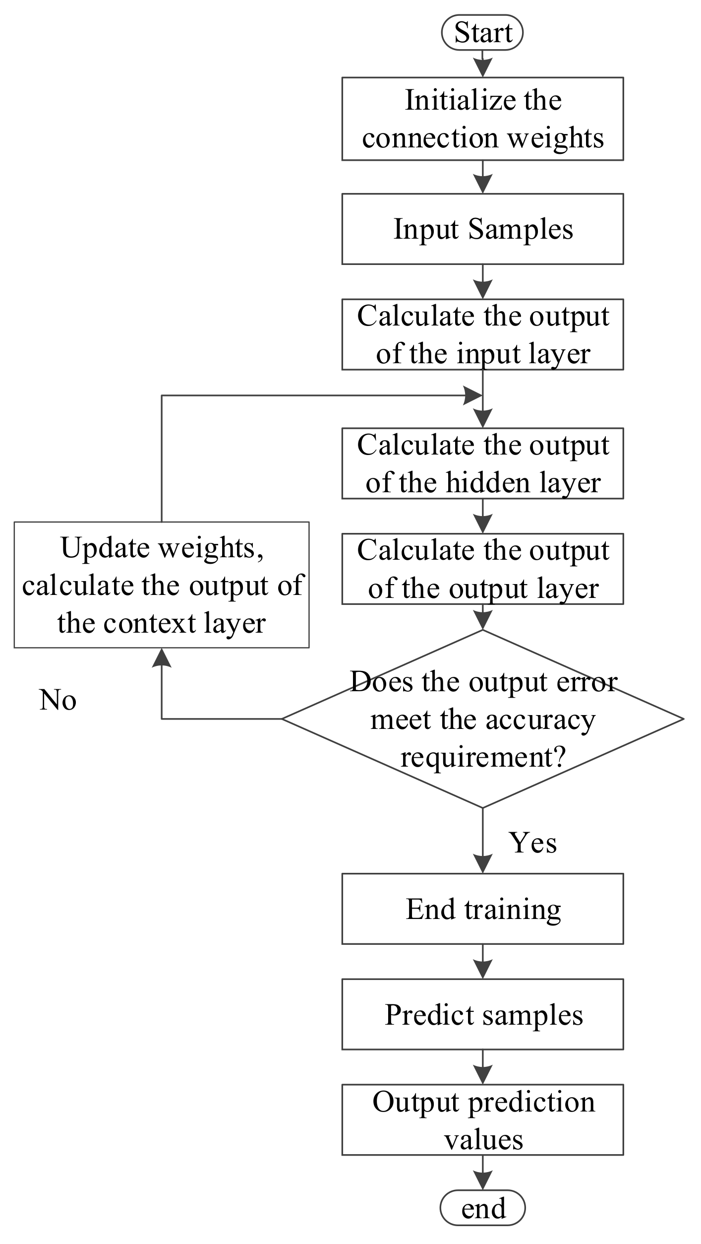
3.2.2. Elman Neural Network (ENN)

ENN is based on the basic structure of the BP neural network and adds a “feedback”. Such an internal feedback network increases its ability to deal with dynamic information of the network itself, which means the system can adapt to the time-varying characteristics and that it is more suitable to establish the forecast model of time series.

ENN includes an input layer, hidden layer, context layer, and output layer. The connection of the input layer, the hidden layer, and the output layer is similar to the BP neural network. The input layer performs signal transmission and the output layer plays a weighting role. The context layer is used to memorize the output value of the hidden layer unit at the previous moment, and is usually considered as a delay operator network. The structure diagram is shown in Figure 3.

The mathematical model of ENN is

$$x\left(k\right)=f({\omega }_1{x}_c\left(k\right)+{\omega }_{2}i(k-1))$$

(8)

$$x_c\left(k\right)=a·x_c(k-1)+x(k-1)$$

(9)

$$y\left(k\right)=g\left({\omega }_{3}x\left(k\right)\right)$$

(10)

where y is the m-dimensional output vector, x is the n-dimensional hidden layer vector, i is the r-dimensional input vector, $x_c$ is the n-dimensional feedback state vector, a is the self-connected feedback gain factor, ${\omega }_1$ is connection weight between the context layer and the hidden layer, ${\omega }_2$ is the connection weight of the input layer and the hidden layer, ${\omega }_3$ is the connection weight of the hidden layer and the output layer, $g(.)$ is the transfer function of the output neuron, and $f(.)$ is the transfer function of the hidden layer neuron.

Like the BP neural network, the number of hidden neurons is the core parameter to determine the model structure. A trial and error process is needed to decide the optimal number of hidden neurons. Once the model structure is settled, the connection weights between different layers are determined by self-learning using the gradient descent method. The training and prediction process by ENN is shown in Figure 4.

3.2.3. Combined Forecasting Model

For the same prediction problem, the optimized combination of multiple different prediction models can effectively improve the prediction accuracy of the model under certain conditions. The combination model development includes three key steps: (1) selection of proper individual models, (2) construction of the mathematical expression of the combination from multiple individual models, and (3) solving the weight of each single model through optimization algorithms.

As the OPT-SVM and ENN are selected here as the candidates for the combined model, the mathematical expressions of the combination model are then supposed to be determined. We focuses on three forms of expressions: linear weighted average, geometric weighted average, and harmonic weighted average; they are expressed as follows:

$$f_{t,c}={\alpha }_1\left(t\right)f_{1,t}+{\alpha }_2\left(t\right)f_{2,t}+\dots +{\alpha }_m\left(t\right)f_{m,t}$$

(11)

$$f_{c,t}=f_{1,t}^{{\alpha }_1\left(t\right)}{f}_{2,t}^{{\alpha }_2\left(t\right)}\dots f_{m,t}^{{\alpha }_m\left(t\right)}$$

(12)

$$f_{c,t}=\frac{1}{\frac{{\alpha }_1\left(t\right)}{f_{1,t}}+\frac{{\alpha }_2\left(t\right)}{f_{2,t}}+\dots +\frac{{\alpha }_m\left(t\right)}{f_{m,t}}}$$

(13)

where t represents the t-th forecast period; $f_c$ is the combined prediction result; $f_1,\dots ,f_m$ are forecast values of m individual prediction models; ${\alpha }_1,\dots ,{\alpha }_m$ are the weights of individual models, respectively; and ${\alpha }_1+{\alpha }_2+\dots +{\alpha }_m=1,{\alpha }_i\ge 0,i=1,2,\dots ,m$.

Solving the time-varying weights Can be regarded as an optimization problem as follows:

$$minQ=Q({\alpha }_1,{\alpha }_2,\dots ,{\alpha }_m),s.t.\left\{\begin{array}{c}{\alpha }_1+{\alpha }_2+\dots +{\alpha }_m=1\\ {\alpha }_i\ge 0,i=1,2,\dots ,m\end{array}\right.$$

(14)

where Q is the objective function that indicates the combined forecast accuracy corresponding to a certain set of weights. In this paper, the Mean absolute percentage error (MAPE) is used as the optimization objective function.

In the t-th forecast period, assign all the data before the t-th period, including simulated values of the modeling period, the predicted values of the forecast period, and the actual measured values of the corresponding period, to Equation (14). Equation (14) is then solved by the sequential quadratic programming method. In the $(t+1)$-th period, the predicted value and measured value of $(t+1)$-th period are incorporated into the known knowledge of the weight solution problem by real-time learning of the latest prediction experience, thereby updating the weights of individual models.

4. Results and Discussion

4.1. Correlation Analysis Results of Meteorological Factors and Daily Load in Four Seasons

Figure 5 shows the correlation analysis results between electric load and meteorological variables. The dependent variable is the electric load, and the independent variables are the meteorological factors. The color bars in the right of each figure represent the range of the correlation coefficient, and the numbers in the figure represent the correlation coefficient. When the correlation coefficient is positive, it shows a trend toward the upper right side; when the correlation coefficient is 1, it is a straight line; when the correlation coefficient is negative, it shows a trend toward the lower left side. The smaller the correlation coefficient, the closer the graph is to a circle. The first row in the figure shows the correlation coefficients between electric load and various meteorological factors. The other rows in the figure are the correlations between various meteorological factors.

It can be seen from the correlation analysis results that the correlation between summer load and meteorological factors the most obvious, followed by autumn and winter loads, and the correlation between spring load and meteorological factors is slightly weaker. In general, air temperature (surface temperature) has the most significant impact on the seasonal load. Besides, among meteorological factors, the correlation between air temperature and the surface temperature reaches 0.9, and the correlation between relative humidity and evaporation in spring, summer, and autumn is also relatively high. It would cause multi-collinearity, which should be carefully treated.

4.2. Analysis of Time-Varying Characteristics of the Resident Load

The total regional power load is composed of three parts: commercial area, industrial area, and residential area, among which the hourly power load of commercial area and industrial area has obvious periodicity, and the influence of environmental factors is relatively small. Resident electric load is difficult to predict due to the influence of people’s lifestyle and weather factors. This paper mainly studies the daily load forecasting, and tries to forecast the hourly residential load with an additional example.

The hourly load of typical daily residents in the four seasons in the region is shown in Figure 6 (select April 15 in spring, August 21 in summer, October 22 in autumn, and February 14 in winter as typical days). It can be seen from the figure that the hourly load characteristics and trends of residents on typical days in different seasons are relatively similar, and the peak load is mainly concentrated at 20 o’clock.

The hourly load trend of residents on a typical day is similar. The peak electricity consumption is mainly concentrated from 17:00 to 22:00. As this period is the time when residents are off work, the load in the residential area reaches the peak of the day.

Due to weather changes, residential areas have increased air conditioning in summer, air conditioning and heating in winter, and the hourly load peak and valley values of residents in summer and winter are higher than those in spring and autumn. The peak difference between summer and spring is about 15 MW. The peak difference in autumn is nearly 20 MW.

4.3. PCA Results of the Meteorological Factors

PCA is conducted on five meteorological variables of temperature, wind speed, relative humidity, evaporation, and surface temperature on a daily scale in the four seasons. The results are presented in

Table 1. The first principal component coefficients and contribution of meteorological factors on daily scales.

Variables	Spring	Summer	Autumn	Winter
Air temperature	0.69	0.43	0.49	0.55
Relative humidity	0.15	−0.44	0.73	0.62
wind speed	−0.09	0.09	0.15	−0.02
Evaporation	0.04	0.54	−0.15	−0.16
Surface temperature	0.70	0.56	0.42	0.54
Contribution/%	49.75	64.06	39.64	41.27

.

Taking winter as an example, the comprehensive meteorological factor (the first principal component) contains 41.27% of information. The normalized variables temperature, relative humidity, and surface temperature have similar coefficient values greater than 0.5, indicating that these three variables are closely related to the meteorological conditions. At the same time, the new factor almost contains the main information of each representative variable, which can be used as a new meteorological feature to represent the meteorological factor. Only the first principal component is used as the comprehensive meteorological factor inputting the proposed model.

4.4. Pre-Ordered Autocorrelation Load Time Lag Results

The autocorrelation function values of daily load in the four seasons are shown in Figure 7. The blue line in the figure represents the critical value of the 95% significance level of the autocorrelation function (the critical value is inversely proportional to the length of the time series). According to the length of the entire load sequence of the four seasons, we checked the critical value table of the correlation coefficient to determine the critical values to be 0.205, 0.209, 0.210, and 0.211. When the autocorrelation function value is greater than the critical value, it indicates that the time lag load is significantly correlated with the target period load; otherwise, the autocorrelation is not significant. The maximum time lag where the positive autocorrelation function value is greater than the critical value is taken as the pre-ordered autocorrelation load time lag. As a result, the pre-ordered autocorrelation load time lag is four days in spring, seven days in summer and autumn, and three days in winter.

4.5. Evaluation Criteria

In this paper, MAPE and maximum absolute percentage error (max APE) are selected to evaluate the predictive performance of the model. The good stability of MAPE can be used as a benchmark for evaluation criteria [35]. They are defined as

$$MAPE=\frac{1}{n}{\sum }_{i=1}^n\frac{|{\widehat{y}}_i-y_i|}{y_i}\times 100\%$$

(15)

$$max\_APE=max(\frac{|{\widehat{y}}_i-y_i|}{y_i}\times 100\%;i=1,2,\dots ,n)$$

(16)

where n is the number of samples, ${\widehat{y}}_i$ is the predicted value, and $y_i$ is the actual value.

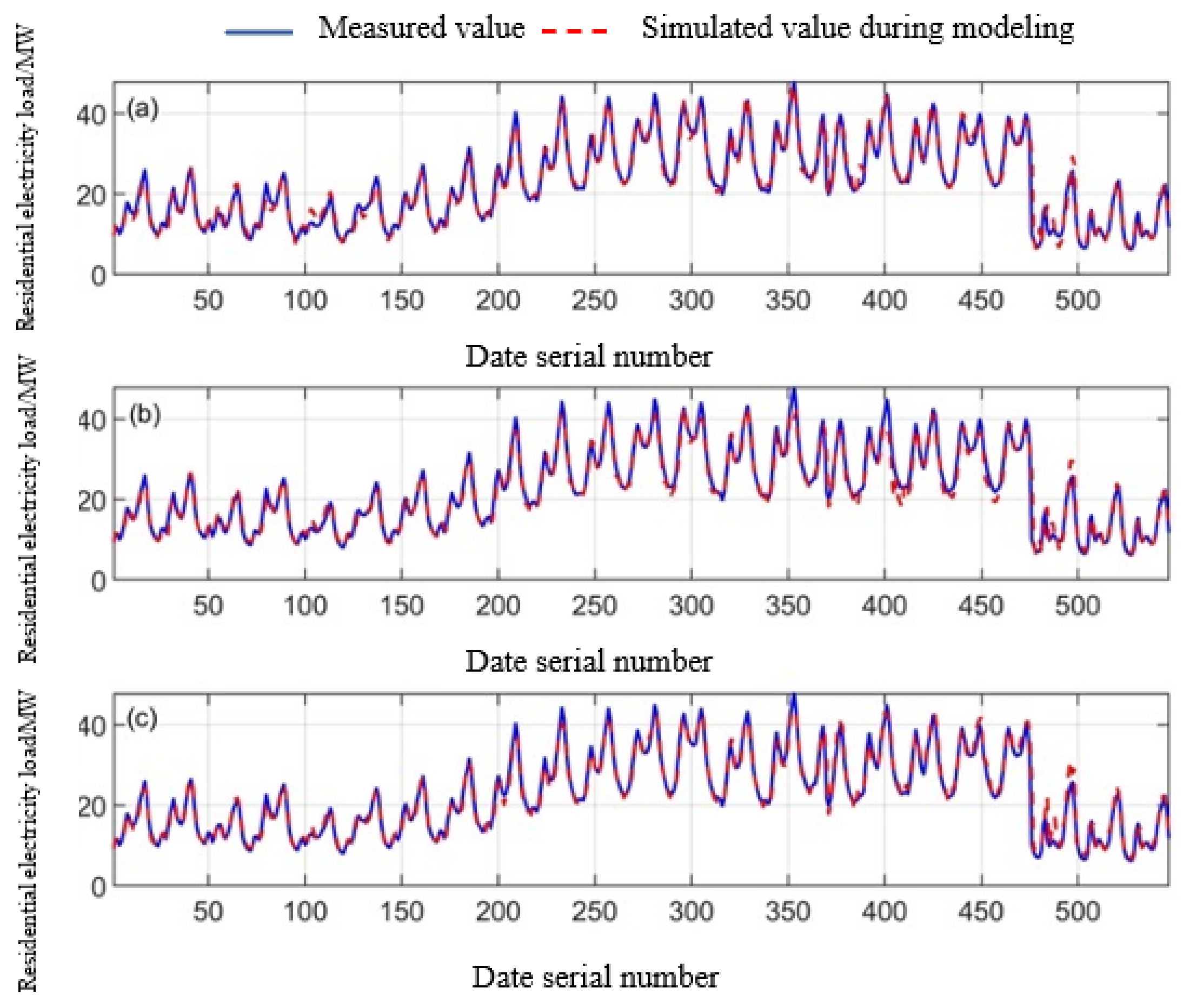
4.6. Load Forecasting Results

First, the forecasting results obtained by individual models are summarized and compared in

Table 2. Forecasting accuracy comparison of OPT-SVM and ENN.

Season	Model	Modeling Stage			Prediction Stage
		Sequence Length (d)	MAPE(%)	max_APE(%)	Sequence Length (d)	MAPE(%)	max_APE (%)
Spring	OPT-SVM	68	1.98	2.90	23	1.96	3.10
	ENN	68	1.08	7.90	23	1.54	8.02
Summer	OPT-SVM	63	3.87	6.29	22	5.69	24.36
	ENN	63	2.69	12.23	22	3.90	26.41
Autumn	OPT-SVM-PCA	63	2.54	4.12	21	1.81	4.15
	ENN	63	1.58	5.85	21	2.04	8.10
Winter	OPT-SVM-PCA	63	3.50	9.70	21	2.80	4.80
	ENN	63	4.28	72.49	21	3.21	9.74

and Figure 8. Figure 8 shows the statistical error results of the OPT-SVM and Elman model for the four-season daily load in simulation period and forecast period. In the figure, the cross x represents the average position, the horizontal line in the box represents the median, the upper and lower boundaries of the box are the 75% and 25% quantiles, and the upper and lower ends of the whiskers line represent the maximum and minimum values except for outliers. It can be seen that for the daily load in spring, summer, and autumn, the average error, 75%, and 25% quantile of ENN are significantly smaller than OPT-SVM; and in winter, the average error and 75% quantile of ENN are larger than that of OPT-SVM. Therefore, ENN has a better forecasting performance for the daily load in spring, summer, and autumn, while OPT-SVM is more suitable for the daily load forecasting in winter.

For the hourly load forecast of residents in summer and winter shown in Figure 9 and Figure 10, the addition of meteorological factors (OPT-SVM-T and OPT-SVM-PCA) to the pre-autocorrelation load helps to improve the prediction accuracy. Here, OPT-SVM-T refers to a load forecasting model that considers the preorder autocorrelation load and adds air temperature as input. Support vector machine model: (1) Load forecasting model (OPT-SVM) that does not consider meteorological variables and takes pre-order autocorrelation load as input; (2) Load forecast model that takes pre-order autocorrelation load and temperature as input (OPT-SVM-T); (3) The load forecasting model (OPT-SVM-PCA) that considers the pre-order load and adds the comprehensive meteorological variable factor (this article uses the first principal component after the principal component analysis of multiple meteorological variables as the comprehensive meteorological factor) as the input. Among them, the use of pre-autocorrelation load and comprehensive weather and OPT-SVM-PCA with the factor as the input has a better forecasting effect on the summer resident load, and the OPT-SVM-T taking into account the temperature factor is more effective for improving the accuracy of the winter resident load forecasting.

• For the hourly load of residents in summer, the Elman-PCA, which adds comprehensive weather factors, has higher accuracy in load forecasting than the other two models. For the hourly load of residents in winter, the Elman-T model has a better application effect.
• For the hourly load of residents in summer and winter, both Elman-PCA and Elman-T are better than the optimized support vector machine model under the same input conditions. Here, Elman-T refers to Elman neural network that considers the pre-order autocorrelation load and adds the temperature as input to the load forecasting model.
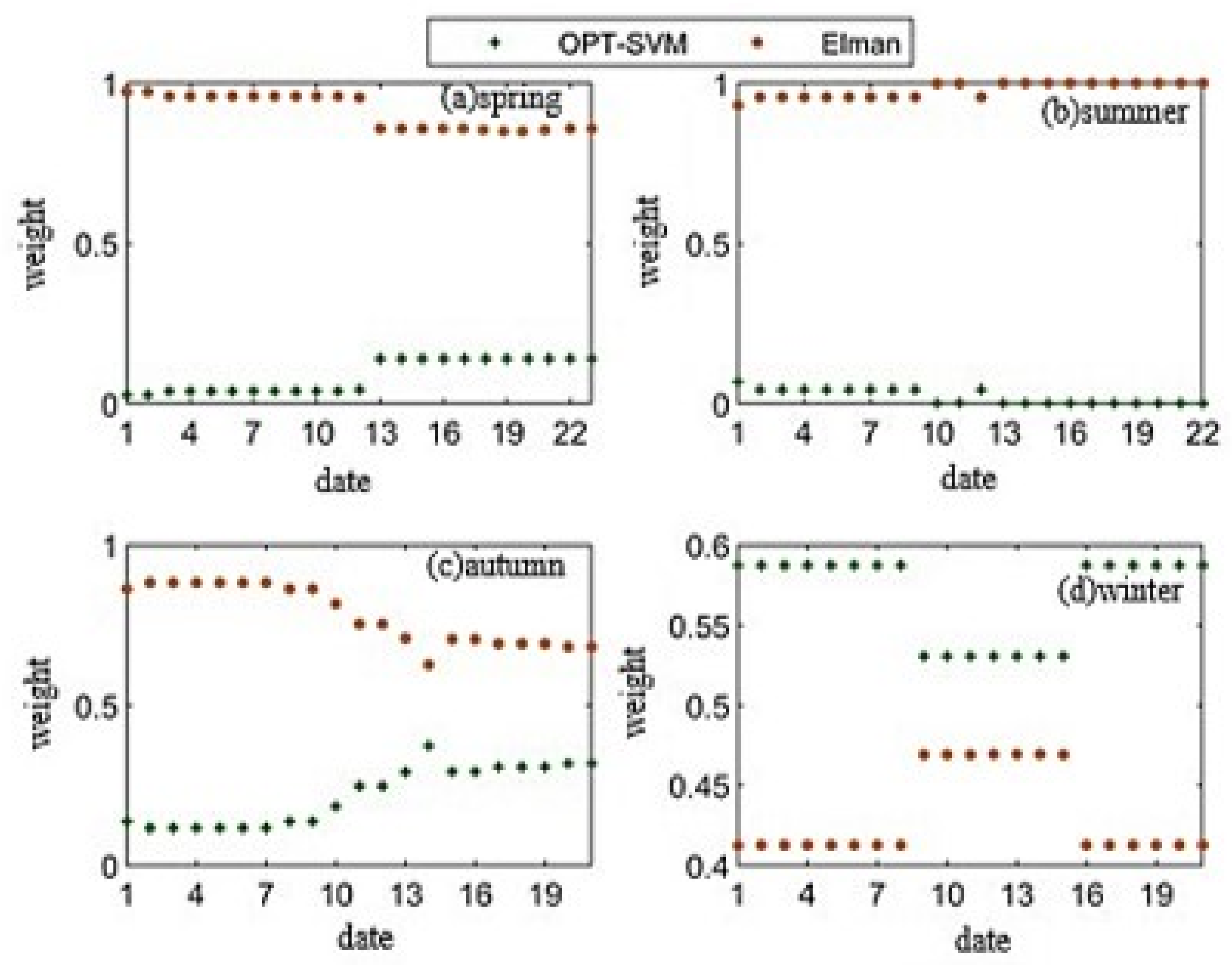
• From the time-by-period error analysis, it is found that the forecast accuracy of the load forecasting model changes with time, and models with lower average forecasting accuracy in a few periods also contain useful information that can help improve the forecasting effect.

The forecast accuracy of the individual models changes over time. Even the models with lower average forecasting accuracy in a few periods also contain useful information that can help improve the forecasting accuracy. As the prediction accuracy of individual models have a good positive correlation with their respective weights, and the weights can also reflect the contribution of the predicted value of each individual model to the combined forecasting model. Based on the results above, we then analyze the time-varying weights of every single model.

Figure 11 shows the time-varying weights of individual models through linear weighted average daily load forecasting in the four seasons. It can be seen from Figure 11 that ENN weights are all higher than OPT-SVM in each forecast period in spring, summer, and autumn, indicating that ENN forecast accuracy is generally higher than OPT-SVM in these three seasons; in winter, the performance of the two prediction model reverses: OPT-SVM has better prediction effect and correspondingly greater weights than ENN. Besides, it can be seen that the time-varying characteristics of the weights of OPT-SVM and ENN in different seasons vary: (1) Before the 13th day in spring, the weights of a single model remain basically stable. After that, the weights of ENN show a small drop while the weights of OPT-SVM increase. (2) During the summer period, the weights of the two models in the combined model have a small change, especially in the late forecast period, the ENN weights stay stable and close to 1. (3) In the autumn forecast period, with the accumulation of forecast experience, the ENN weights slowly decrease while OPT-SVM weights increase accordingly. (4) The ENN weights and OPT-SVM weights in the winter forecast period are between 0.4–0.5 and 0.5–0.6, respectively. According to the time-varying characteristics, ENN weights and OPT-SVM weights can be divided into three segments in winter, and both weights in the middle segment are getting closer.

Figure 12 shows the time-varying weights of individual models through harmonic weighted average daily load forecasting in the four seasons. Comparing Figure 11, we can see that although the mathematical expressions of the combined prediction are different, the time-varying characteristics of the weights of ENN and OPT-SVM have not changed significantly. Due to space limitations, the time-varying weights of the geometric weighted average method are no longer given.

Finally, the prediction accuracy of the individual models and combined models is compared in

Table 3. Prediction result comparison of the individual models and combined models.

Season	Model	Prediction Sequence Length	MAPE/%	max_APE/%
Spring	OPT-SVM	23	1.96	2.88
	ENN	23	1.54	7.53
	Linear weighted average	23	1.49	7.34
	Geometric weighted average	23	1.49	7.34
	Harmonic weighted average	23	1.48	7.34
Summer	OPT-SVM	22	5.68	22.59
	ENN	22	3.80	25.01
	Linear weighted average	22	3.82	25.01
	Geometric weighted average	22	3.82	25.00
	Harmonic weighted average	22	3.81	25.01
Autumn	OPT-SVM	21	1.80	3.96
	ENN	21	2.03	7.57
	Linear weighted average	21	1.85	5.93
	Geometric weighted average	21	1.86	5.94
	Harmonic weighted average	21	1.87	5.95
Winter	OPT-SVM	21	2.80	4.25
	ENN	21	3.20	9.31
	Linear weighted average	21	2.54	6.10
	Geometric weighted average	21	2.55	6.23
	Harmonic weighted average	21	2.56	6.35

. The following observations have been noted. (1) For load forecasting in spring, the MAPEs and maxAPEs of the three combined forecasting models are generally close to each other; the MAPEs of the three combined models are lower than that of OPT-SVM and ENN, and the maxAPEs of combined models are between two individual models. (2) For the daily load forecasting in summer, the MAPEs and maxAPEs of the three combined models are close to or slightly lower than that of OPT-SVM and ENN. (3) For the daily load forecasting in autumn, the MAPEs and maxAPEs of the combined models for daily load forecast are both greater than the individual models. (4) In winter, the combined forecasting models significantly decrease the MAPEs while the maxAPEs of the combined models are between that of OPT-SVM and ENN.

We further rank the prediction errors of five models in each prediction period. Figure 13 shows the ranking results. The smaller the blue circle in the figure, the smaller the absolute percentage error. As shown in Figure 13, the number of periods with the smallest forecast error of the harmonic weighted average method is significantly higher than the other two combined forecasting models. Based on the above analysis, it can be concluded that the harmonic weighted average is the best model among the three combined models for daily load forecasting of the four seasons. For the daily load forecasting in spring and winter, the combined model can be used to archive better performance than a single model; for the daily load forecasting in summer, the accuracy of the combined models is basically the same as that of the individual models; for the daily load forecasting in autumn, the prediction accuracy of the combined models is between OPT-SVM and ENN.

Further research on the forecasting accuracy improvement of the combined model in each time period is of great significance for deepening the understanding of the effectiveness of combined forecasting. Figure 14 shows the forecast accuracy of the combined models for the total daily load of the four seasons compared with the single models. As can be seen from the Figure 14, compared with OPT-SVM, the harmonic weighted average has a positive error reduction value for multiple periods when predicting the total daily load in spring, and finally shows a greater improvement in the average prediction accuracy of OPT-SVM. Compared with Elman, only a few time period errors have been slightly reduced. At the same time, some time periods are affected by OPT-SVM, and the error is slightly increased. The combined effect causes the harmonic weighted average to be smaller than the OPT-SVM average error. For the total load of autumn, although the forecast error in some periods has also been effectively improved, the errors in the two periods are significantly increased, which means the average accuracy of the harmonic weighted average forecast is worse than OPT-SVM. Based on the above analysis, it can be seen that the improvement of the average forecast accuracy of the combined forecasting model can roughly reflect the overall situation of the forecast error reduction in each period. When the average forecasting accuracy is improved, it can be trusted that the combined forecasting model can get closer to the actual measurement in more time periods. When the average prediction accuracy is worse than the optimal single model, it can be considered how to make full use of the partial error to obtain the prediction result of the compressed period, so as to provide useful guidance for further improving the prediction accuracy.

5. Conclusions

Electric load forecasting plays an important role in the power system. In order to balance the supply and demand of power system in integrated energy, it is necessary to establish a scientific model for power load forecasting. This paper takes an industrial park in Nantong as an example and establishes forecasting models that consider meteorological factors.

This paper establishes a prediction model considering meteorological factors, including an optimization vector machine model, Elman neural network model, and time-varying weight combination prediction model, that studies the impact of meteorological factors on power load forecasting and evaluates the applicability of the model. Based on the analysis of the variation characteristics of regional power load in different seasons and typical days, the correlation between meteorological factors such as temperature, relative humidity, wind speed, evaporation and surface temperature, and load is analyzed, so as to provide basis for selecting key meteorological factors. From the analysis results, the temperature has the greatest impact on the load in four seasons.

When the average forecasting accuracy is improved, the combined forecasting models can obtain prediction results closer to the actual measured values in more periods. The results show that the harmonic weighted average method is recommended for the optimal combined forecasting model. The first mock exam is better than the first mock exam model, especially for the total load in spring and winter. The average absolute percentage error (MAPE) of the forecast is lower than that of the single model.

Improving the accuracy of short-term regional power load forecasting is a long-term work. Its forecasting models are diverse and the influencing factors are very complex. This paper only analyzes the impact of some meteorological factors on short-term load forecasting. In the field of power load forecasting, whether from the exploration of load forecasting model or the comprehensive consideration of influencing factors, there are still many research contents and methods worthy of further test, which can be studied and analyzed from the following perspectives:

• In this paper, considering the influence of meteorological factors, in the follow-up research, we can take into account the plot type, week type, and cultural activities, and establish a joint model with multiple influencing factors to investigate the impact of comprehensive influencing factors on regional short-term power load.
• The follow-up research can consider prediction models and methods to make intelligent prediction for more different regions, different utilization types, and different environmental factors.

References

1. Raza, M.Q.; Khosravi, A. A review on artificial intelligence based load demand forecasting techniques for smart grid and buildings. Renew. Sustain. Energy Rev. 2015, 50, 1352–1372. [Google Scholar] [CrossRef]
2. Fahad, M.U.; Arbab, N. Factor affecting short term load forecasting. J. Clean Energy Technol. 2014, 2, 305–309. [Google Scholar] [CrossRef]
3. Khatoon, S.; Singh, A.K. Effects of various factors on electric load forecasting: An overview. In Proceedings of the 2014 6th IEEE Power India International Conference (PIICON), Delhi, India, 5–7 December 2014; pp. 1–5. [Google Scholar]
4. Amjady, N. Short-term hourly load forecasting using time-series modeling with peak load estimation capability. IEEE Trans. Power Syst. 2001, 16, 498–505. [Google Scholar] [CrossRef]
5. Božić, M.; Stojanović, M.; Stajić, Z.; Floranović, N. Mutual information-based inputs selection for electric load time series forecasting. Entropy 2013, 15, 926–942. [Google Scholar] [CrossRef]
6. Pappas, S.S.; Ekonomou, L.; Karampelas, P.; Karamousantas, D.C.; Katsikas, S.K.; Chatzarakis, G.E.; Skafidas, P.D. Electricity demand load forecasting of the hellenic power system using an arma model. Electr. Power Syst. Res. 2010, 80, 256–264. [Google Scholar] [CrossRef]
7. Goia, A.; May, C.; Fusai, G. Functional clustering and linear regression for peak load forecasting. Int. J. Forecast. 2010, 26, 700–711. [Google Scholar] [CrossRef]
8. Liao, N.; Hu, Z.; Ma, Y.; Lu, W. Review of the short-term load forecasting methods of electric power system. Power Syst. Prot. Control 2011, 39, 147–152. [Google Scholar]
9. Park, D.C.; El-Sharkawi, M.A.; Marks, R.J.; Atlas, L.E.; Damborg, M.J. Electric load forecasting using an artificial neural network. IEEE Trans. Power Syst. 1991, 6, 442–449. [Google Scholar] [CrossRef] [Green Version]
10. Nose-Filho, K.; Lotufo, A.D.P.; Minussi, C.R. Short-term multinodal load forecasting using a modified general regression neural network. IEEE Trans. Power Deliv. 2011, 26, 2862–2869. [Google Scholar] [CrossRef]
11. Viegas, J.L.; Vieira, S.M.; Melício, R.; Mendes, V.M.F.; Sousa, J.M.C. Ga-ann short-term electricity load forecasting. In Doctoral Conference on Computing, Electrical and Industrial Systems; Springer: Berlin/Heidelberg, Germany, 2016; pp. 485–493. [Google Scholar]
12. Ho, K.-L.; Hsu, Y.-Y.; Chen, C.-F.; Lee, T.-E.; Liang, C.-C. Tsau-Shin Lai, and Kung-Keng Chen. Short term load forecasting of taiwan power system using a knowledge-based expert system. IEEE Trans. Power Syst. 1990, 5, 1214–1221. [Google Scholar]
13. Mohandes, M. Support vector machines for short-term electrical load forecasting. Int. J. Energy Res. 2002, 26, 335–345. [Google Scholar] [CrossRef]
14. Wang, J.; Zhou, Y.; Chen, X. Electricity load forecasting based on support vector machines and simulated annealing particle swarm optimization algorithm. In Proceedings of the 2007 IEEE International Conference on Automation and Logistics, Jinan, China, 18–21 August 2007; pp. 2836–2841. [Google Scholar]
15. Pai, P.-F.; Hong, W.-C. Forecasting regional electricity load based on recurrent support vector machines with genetic algorithms. Electr. Power Syst. Res. 2005, 74, 417–425. [Google Scholar] [CrossRef]
16. Niu, D.; Wang, Y.; Wu, D.D. Power load forecasting using support vector machine and ant colony optimization. Expert Syst. Appl. 2010, 37, 2531–2539. [Google Scholar] [CrossRef]
17. Li, W.-Q.; Chang, L. A combination model with variable weight optimization for short-term electrical load forecasting. Energy 2018, 164, 575–593. [Google Scholar] [CrossRef]
18. Bates, J.M.; Granger, C.W.J. The combination of forecasts. J. Oper. Res. Soc. 1969, 20, 451–468. [Google Scholar] [CrossRef]
19. Zhou, D.-Q.; Wu, B.-L. Optimization and power load forecasting of gray bp neural network model. Power Syst. Prot. Control 2011, 39, 65–69. [Google Scholar]
20. Xiao, L.; Shao, W.; Liang, T.; Wang, C. A combined model based on multiple seasonal patterns and modified firefly algorithm for electrical load forecasting. Appl. Energy 2016, 167, 135–153. [Google Scholar] [CrossRef]
21. Liu, Z. Short-Term Load Forecasting Based on Chaos Theory and Support Vector Machine. Master’s Thesis, Yanshn University, Qinhuangdao City, China, 2017. [Google Scholar]
22. Zhang, J.; Wei, Y.-M.; Li, D.; Tan, Z.; Zhou, J. Short term electricity load forecasting using a hybrid model. Energy 2018, 158, 774–781. [Google Scholar] [CrossRef]
23. Singh, P.; Dwivedi, P. Integration of new evolutionary approach with artificial neural network for solving short term load forecast problem. Appl. Energy 2018, 217, 537–549. [Google Scholar] [CrossRef]
24. Tian, C.; Hao, Y. A novel nonlinear combined forecasting system for short-term load forecasting. Energies 2018, 11, 712. [Google Scholar] [CrossRef] [Green Version]
25. Elattar, E.E.; Sabiha, N.A.; Alsharef, M.; Metwaly, M.K.; Abd-Elhady, A.M.; Taha, I.B.M. Short term electric load forecasting using hybrid algorithm for smart cities. Appl. Intell. 2020, 50, 3379–3399. [Google Scholar] [CrossRef]
26. Sun, C.; Lyu, Q.; Zhu, S.; Zheng, W.; Cao, Y.; Wang, J. Ultra-short-term Power Load Forecasting Based on Two-layer XGBoost Algorithm Considering the Influence of Multiple Features. High Volt. Eng. 2021, 47, 2885–2898. [Google Scholar]
27. Jin, C.; Lu, X.; Xu, Y.; Liu, R.; Zhang, J. Short-term Load Forecasting Based on Similar Days and Multi-integration Combination. CSU-EPSA. Available online: https://kns.cnki.net/kcms/detail/detail.aspx?doi=10.19635/j.cnki.csu-epsa.000814 (accessed on 30 August 2021).
28. Wang, S.; Zhang, Z. Short-term Load Forecasting of Power System Based on Quantum Weighted GRU Neural Network. CSU-EPSA. Available online: https://kns.cnki.net/kcms/detail/detail.aspx?doi=10.19635/j.cnki.csu-epsa.000804 (accessed on 30 August 2021).
29. Xu, X.; Zhao, Y.; Liu, Z.; Li, L.; Lu, Y. Daily Load Characteristic Classification and Feature Set Reconstruction Strategy for Short-term Power Load Forecasting. Power Syst. Technol. Available online: https://kns.cnki.net/kcms/detail/11.2410.TM.20210705.0939.001.html (accessed on 30 August 2021).
30. Wang, J.; Zheng, J.; Wang, X.; Yu, J. Research on Power System Load Forecasting Based on Improved Deep Belief Network. CSU-EPSA. Available online: https://kns.cnki.net/kcms/detail/detail.aspx?doi=10.19635/j.cnki.csu-epsa.000781 (accessed on 30 August 2021).
31. Cao, Y.; Zhang, Z.J.; Zhou, C. Data processing strategies in short term electric load forecasting. In Proceedings of the 2012 International Conference on Computer Science and Service System, Nanjing, China, 11–13 August 2012; pp. 174–177. [Google Scholar]
32. Guo, X.-C.; Chen, Z.-Y.; Ge, H.-W.; Liang, Y.-C. Short-term load forecasting using neural network with principal component analysis. In Proceedings of the 2004 International Conference on Machine Learning and Cybernetics (IEEE Cat. No. 04EX826), Shanghai, China, 26–29 August 2004; Volume 6, pp. 3365–3369. [Google Scholar]
33. Sood, R.; Koprinska, I.; Agelidis, V.G. Electricity load forecasting based on autocorrelation analysis. In Proceedings of the 2010 International Joint Conference on Neural Networks (IJCNN), Barcelona, Spain, 18–23 July 2010; pp. 1–8. [Google Scholar]
34. Sudibyo, S.; Murat, M.N.; Aziz, N. Simulated annealing-particle swarm optimization (sa-pso): Particle distribution study and application in neural wiener-based nmpc. In Proceedings of the 2015 10th Asian Control Conference (ASCC), Kota Kinabalu, Malaysia, 31 May–3 June 2015; pp. 1–6. [Google Scholar]
35. Kong, X.; Li, C.; Zheng, F.; Wang, C. Improved deep belief network for short-term load forecasting considering demand-side management. IEEE Trans. Power Syst. 2019, 35, 1531–1538. [Google Scholar] [CrossRef]
Figure 1. Daily load curve of the studied park.
Processes 09 01617 g001
Figure 2. Framework of the proposed method.
Processes 09 01617 g002
Figure 3. The structure of Elman Neural Network.
Processes 09 01617 g003
Figure 4. The flowchart of electrical load forecast by ENN.
Processes 09 01617 g004
Figure 5. Correlation analysis of daily load and meteorological factors in different seasons. (a) Spring (March 1 to June 3); (b) Summer (June 4 to September 3); (c) Autumn (September 4 to December 3); (d) Winter (December 4 to February 28 of the following year).
Processes 09 01617 g005aProcesses 09 01617 g005b
Figure 6. Hourly load changes of typical daily residents in an industrial park in different seasons.
Processes 09 01617 g006
Figure 7. ACF of daily load in four seasons.
Processes 09 01617 g007
Figure 8. Statistical chart of total load error in four seasons. (a); Spring (March 1 to June 3); (b) Summer (June 4 to September 3); (c) Autumn (September 4 to December 3); (d) Winter (February 4 to February 28 of the following year).
Processes 09 01617 g008
Figure 9. Optimized support vector machine model to predict the hourly load of residents in winter: (a) OPT-SVM (b) OPT-SVM-T (c) OPT-SVM-PCA.
Processes 09 01617 g009
Figure 10. Hourly power load forecasting in residential area in summer: (a) OPT-SVM (b) OPT-SVM-T (c) OPT-SVM-PCA.
Processes 09 01617 g010
Figure 11. Time-varying weights of individual models through linear weighted average daily load forecasting.
Processes 09 01617 g011
Figure 12. Time-varying weights of individual models through harmonic weighted average daily load forecasting.
Processes 09 01617 g012
Figure 13. Prediction error ranking results for each period with different models. (a) Spring (March 1 to June 3); (b) Summer (June 4 to September 3); (c) Autumn (September 4 to December 3); (d) Winter (December 4 to February 28 of the following year).
Processes 09 01617 g013
Figure 14. The forecast error reduction effects of the combined model by harmonic weighted average compared with the single models. (a) Spring (March 1 to June 3); (b) Summer (June 4 to September 3); (c) Autumn (September 4 to December 3); (d) Winter (December 4 to February 28 of the following year).
Processes 09 01617 g014