Approximation Possibilities of Fuzzy Control Surfaces for Purpose of Implementation into Microcontrollers

Abstract

The main contribution of the paper is the simplification of the computational process of fuzzy control of a mobile robot controlled by a microcontroller. We present a way to implement this control method with a reduced computation time of control actions and memory demand. Our way to accomplish this, was to replace the fuzzy controller with the approximation of its resulting control surfaces. In the paper, we use the previously presented approximation by the table and describe other methods of approximation of the control area through polynomial and exponential function. We tested all approximation methods in simulations and with a real mobile robot. Based on the measured trajectory of the EN20 mobile robot, we found that approximation through the table is the most accurate in terms of the fuzzy surface but delivers noticeable oscillations of mobile robot control in real conditions. Polynomial and exponential functions fuzzy surface approximations were less accurate than the table, but provide smoother control based on robot trajectories and are much more appropriate in terms of microcontroller implementation due to lower demand on memory.

1. Introduction

The potential for using autonomous mobile robotics in practice is constantly increasing and demand for autonomous systems continues. Complex systems require intelligent control algorithms to perform precisely. One of such algorithms is fuzzy control [1]. The theory of fuzzy sets has revolutionized many applications unsolvable by traditional control theory [2]. This is one of the reasons for adopting fuzzy control in the field of unstructured, dynamically changing environments [3]. Fuzzy sets theory was practically applied in the field of control by Mamdani and Takagi-Sugeno and later further developed by Karnik-Mendel and Wu-Mendel. However, these approaches are due to calculation complexity very demanding on hardware, in particular for control problems [4]. The first advantage of the fuzzy controller is the ability to control simultaneously multiple variables as was demonstrated in the design of omnidirectional mobile robot navigation [5]. The second advantage, specific to fuzzy control, is that it is not required to know the mathematical model of the controlled system [6,7]. This can be problematic with most of the linearization–based and algebraic control algorithms when the dynamic system cannot be described for some reason. Therefore, in those cases, an appropriate choice is to use control methods capable of dealing with uncertainties, such as fuzzy logic [1].

In mobile robotics, the most desired control tasks are trajectory tracking, path following, or moving to a specific position. Many authors developed trajectory tracking algorithms based on the dynamic properties of controlled systems [8,9]. Some of them also consider control action constraints for the actuators [10,11]. But from the implementation point of view, these algorithms are very dependent on the exact mathematical description of the system. Therefore, it is more appropriate to explore and improve the possibilities of fuzzy control for wider use. Numerous researchers used fuzzy logic to investigate its behavior and usability in the field of controlling autonomous mobile robots. Based on the results of [12], fuzzy logic controllers showed an ability to process data from multiple inputs and to lead robots to their destination. Authors Faisal et al. [13] used a synthesis of two fuzzy controllers for mobile robot navigation in the warehouse. A recent paper by Štefek et al. [14] showed the usage of genetic algorithms for fuzzy controller optimization. The optimized controller outperformed all compared controllers. The control quality is mainly influenced by the number of fuzzy membership functions and fuzzy inference rules [15]. Furthermore, with an appropriate selection of fuzzy membership functions shapes and rules formulation, better control results can be obtained [16]. On the other hand, with an increasing number of rules, memory allocation becomes the most limiting factor and execution time is also increased [17]. Given that, computers, programmable logic controllers, or digital signal processors are used to providing fast sampling periods. Their disadvantage is mainly high price and higher power consumption. Therefore, it is suitable to use a microcontroller as a central control unit of a system like a mobile robot when these factors need to be considered.

In numerous presented applications fuzzy control is used with microcontrollers. Work [18] presented temperature and humidity control, in work [19] fuzzy control was used for pressure control, and also for electric motor control in [20]. Papers by [21,22] presented control of small mobile robots. In all referred papers, results showed that microcontrollers are suitable for implementation purposes of fuzzy logic techniques when the fuzzy controller has not too many fuzzy inference rules and sample times in milliseconds are not required. This is supported by [18]. The main limitations of microcontrollers are limited computing power, memory, and still limited possibilities for direct fuzzy control implementation for commercially available microcontrollers. This means that the possibilities of implementing fuzzy control into microcontrollers are still limited due to high requirements on computing power required by fuzzy logic algorithms [23]. For this reason, our work is devoted to additional possibilities of approximation of fuzzy control surfaces into the control system of the mobile robot. Another presented approach by Sekaj [24] has proposed a method for defuzzification approximation, similar to fuzzy logic but without explicitly using fuzzy logic. The most recent paper on this topic presented a new type of fuzzy membership function that provides a computationally efficient defuzzification process [25]. Work [26] showed an interesting solution to cope with the slow execution time of the controller. An approximation of fuzzy control surfaces through lookup tables was used.

Inspired by this approach to directly implement fuzzy control surfaces, in this paper we present a way to use polynomial and exponential functions for fuzzy control surface approximation. Moreover, we compare these two methods to the table approximation. The control accuracy of the approximations will be analyzed using both simulations of a mathematical model of a mobile robot and the real mobile robot EN20.

This paper is organized as follows. In Section 2 materials and methods are presented. A comparison of the proposed fuzzy controller along with created approximation is addressed in Section 3. The discussion and conclusions are given in Section 4 and Section 5.

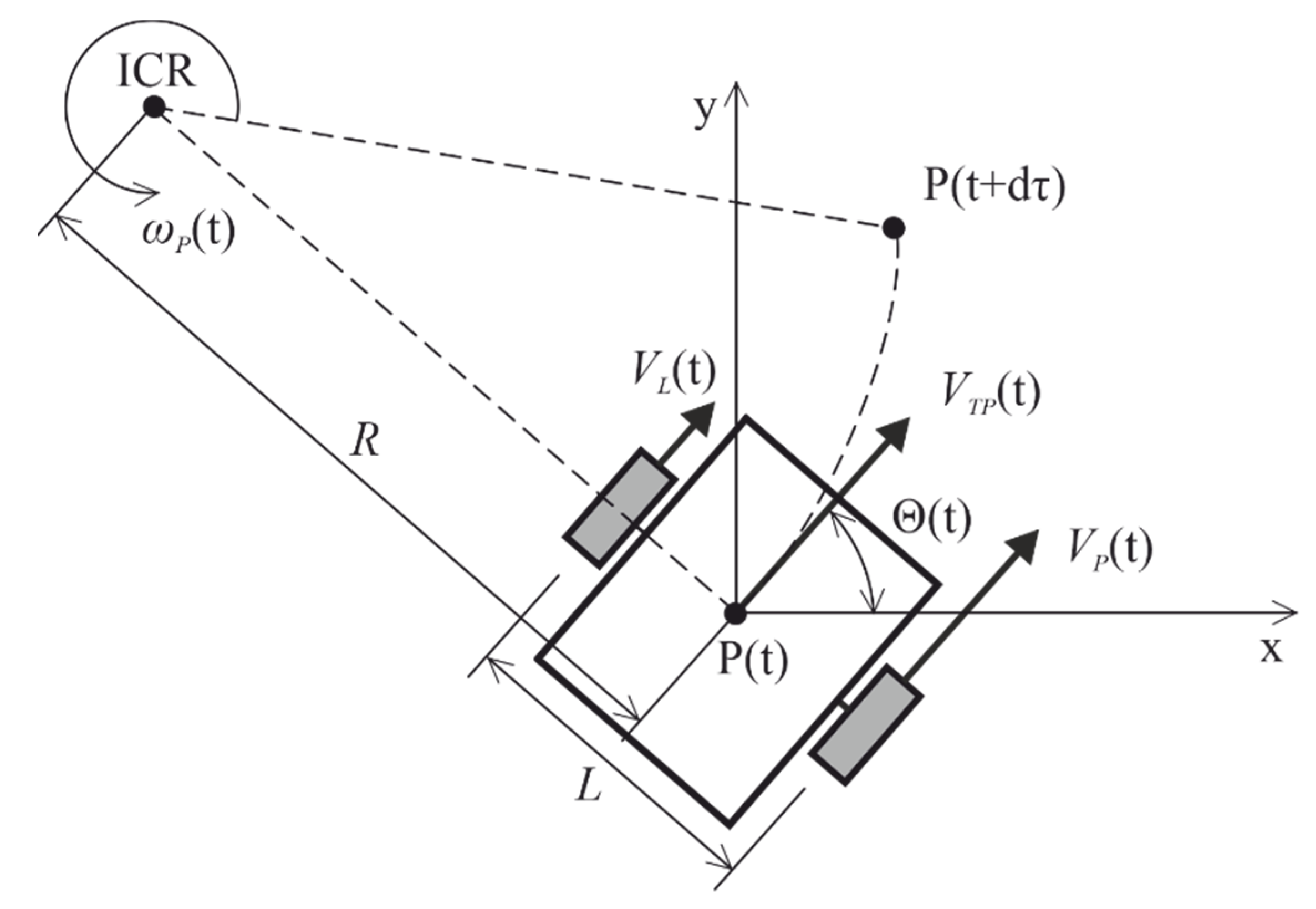
2. Differential Drive Kinematics

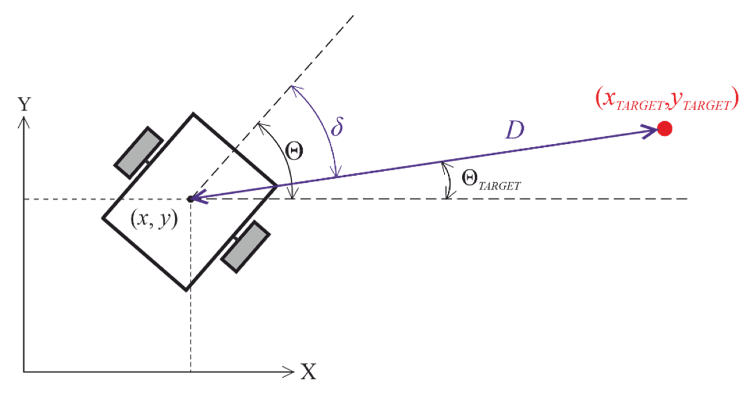
Differential drive chassis is characterized by two independently driven wheels located on the common axis and often the third supportive wheel. Distance between the driven wheels is called track width, L as shown in Figure 1. The movement can be described as a movement along the arcs around the instant center of rotation (ICR) with the radius of R. From Figure 1, the simplest will be to calculate the position of the chassis relative to the P point, which lies in the center of the wheel axis.

Angular velocity of the robot ω_P is calculated from the difference in the speeds of the left and right wheel from (1) [27]:

$${\omega }_P\left(t\right)=\frac{V_P\left(t\right)-V_L\left(t\right)}{L}$$

(1)

where L is track width, V_P and V_L is peripheral velocity of right V_P and left V_L wheels are given in (2) [27]:

$$\begin{array}{l}{V}_P\left(t\right)=w_P\left(t\right)\left(R+\frac{L}{2}\right)\\ V_L\left(t\right)={\omega }_P\left(t\right)\left(R-\frac{L}{2}\right)\end{array}$$

(2)

where R is radius to the instant center of rotation. To determine tangential speed V_TP of the chassis at the point P from the peripheral velocities of wheels we simply calculate their mean value (3) [27]:

$$V_{TP}\left(t\right)=\frac{V_P\left(t\right)+V_L\left(t\right)}{2}$$

(3)

From the V_P and V_L it is possible to determine the position of differential drive chassis in the Cartesian coordinate system based on the previous values as the system of difference equations to be used in discrete system (4):

$$\begin{array}{l}\mathsf{\Theta }\left(k\right)=\frac{V_P\left(k\right)-V_L\left(k\right)}{L}T+\mathsf{\Theta }\left(k-1\right)\\ x\left(k\right)=\frac{V_P\left(k\right)+V_L\left(k\right)}{2}\cos \left[\mathsf{\Theta }\left(k\right)\right]·T+x\left(k-1\right)\\ y\left(k\right)=\frac{V_P\left(k\right)+V_L\left(k\right)}{2}\sin \left[\mathsf{\Theta }\left(k\right)\right]·T+y\left(k-1\right)\end{array}$$

(4)

where x(k), y(k) is current sample of the x and y mobile robot coordinates, x(k − 1) and y(k − 1) is the previous sample of the x and y mobile robot coordinates, Θ(k) is current angle of the robot, Θ(k − 1) is the previous angle of the robot, V_P(k) and V_L(k) is current sample of the right and left wheel peripheral velocity and T is the sampling period [27].

2.1. Control Task

Based on the distance of the mobile robot from the target position D and the angle of deflection of the mobile robot from the target position of the mobile robot δ, the task of a fuzzy controller is to control the speed of the right and left wheel of the EN20 mobile robot so that the mobile robot reaches its target position in the shortest possible time and with as little deviation from the direct direction as possible. The calculation of the distance of mobile robot from the target position D is given by (5) [27]:

$$D=\sqrt{{\left(x-x_{TARGET}\right)}^2+{\left(y-y_{TARGET}\right)}^2}$$

(5)

where x_TARGET, y_TARGET is position of target point, x and y are current coordinates of the mobile robot. Deflection angle is derived from the difference between robot’s angle and the desired angle to the target point in (6) [27]:

$$\begin{array}{l}{\mathsf{\Theta }}_{TARGET}=\left(arcsin\frac{y_{TARGET}-y}{D}\right)\\ \delta =\left(\mathsf{\Theta }-{\mathsf{\Theta }}_{TARGET}\right)\frac{180}{\pi }\end{array}$$

(6)

where Θ_TARGET is desired angle to the target point and δ is deflection angle of mobile robot from the target. These input quantities of our fuzzy controller are for better understanding shown in Figure 2.

Furthermore, if we in (5,6) replace the constant coordinate y_TARGET by function y_TARGET = f(x), where f(x) represents trajectory function, then the robot can move along the defined trajectory by this function. This solution is limited to trajectories, where for each x-coordinate is only one y-coordinate.

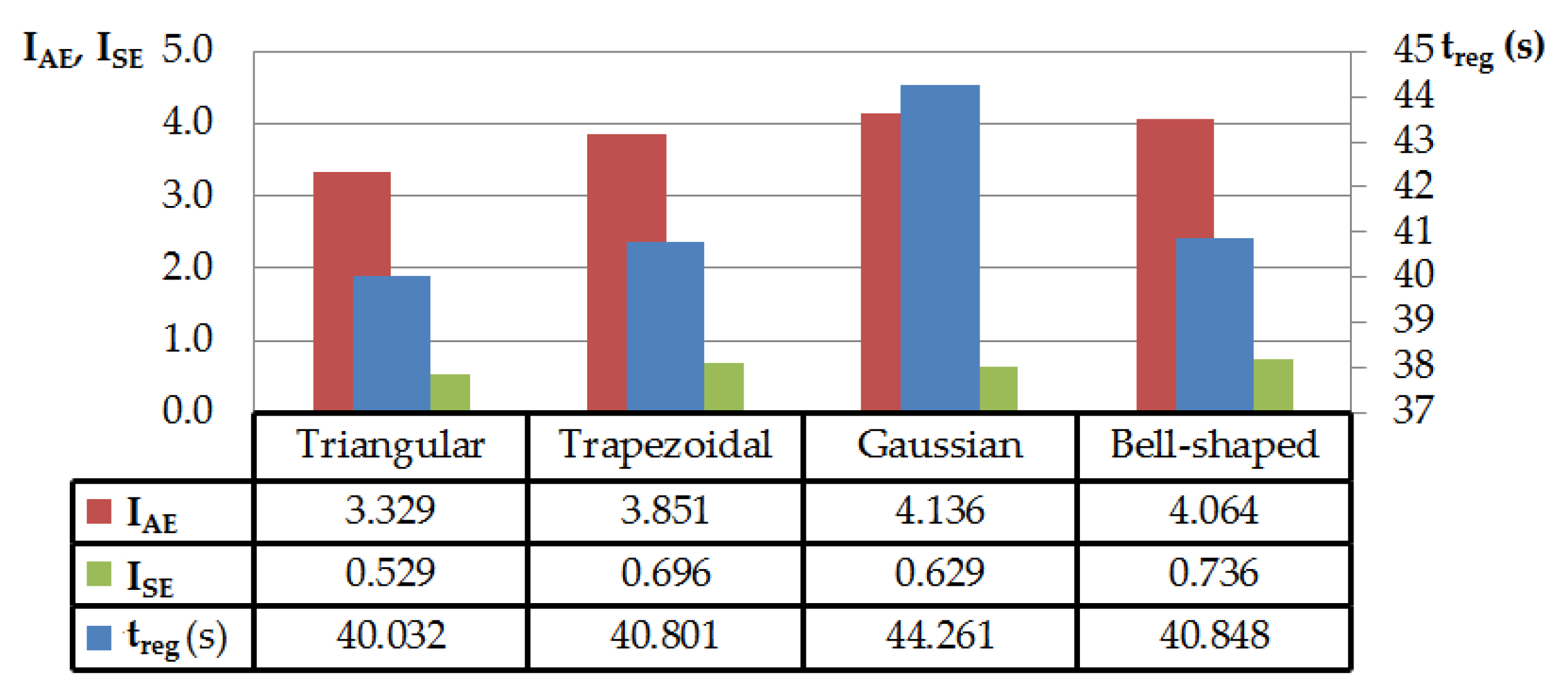
2.2. Control Quality Criterions

For determining the deviation of the robot from straight path to the target position we use general control quality criterions—absolute and quadratic error control area. Absolute error control area I_AE in (7) is suitable for oscillating process variable error values and property of squared error control area I_SE in (8) is accentuation of large error values and neglecting small error values.

$$I_{AE}=\underset{0}{\overset{\infty }{{\displaystyle \int }}}\left|e\left(t\right)\right|dt$$

(7)

$$I_{SE}=\underset{0}{\overset{\infty }{{\displaystyle \int }}}e{\left(t\right)}^{2}dt$$

(8)

In our case the control error e(t) is the actual deviation of the mobile robot from the line connecting the starting and target point. The aim is to achieve the smallest error control areas I_AE and I_SE. The closer they are to zero, the more the ideal trajectory is tracked. Error area is area bordered by measured trajectory of the robot and line between start and the target points. Another important criterion is control time t_reg defined as time interval from the first change of control variable to the setpoint reached within a defined tolerance [23]. In this work it represents time during the mobile robot reaches its target position.

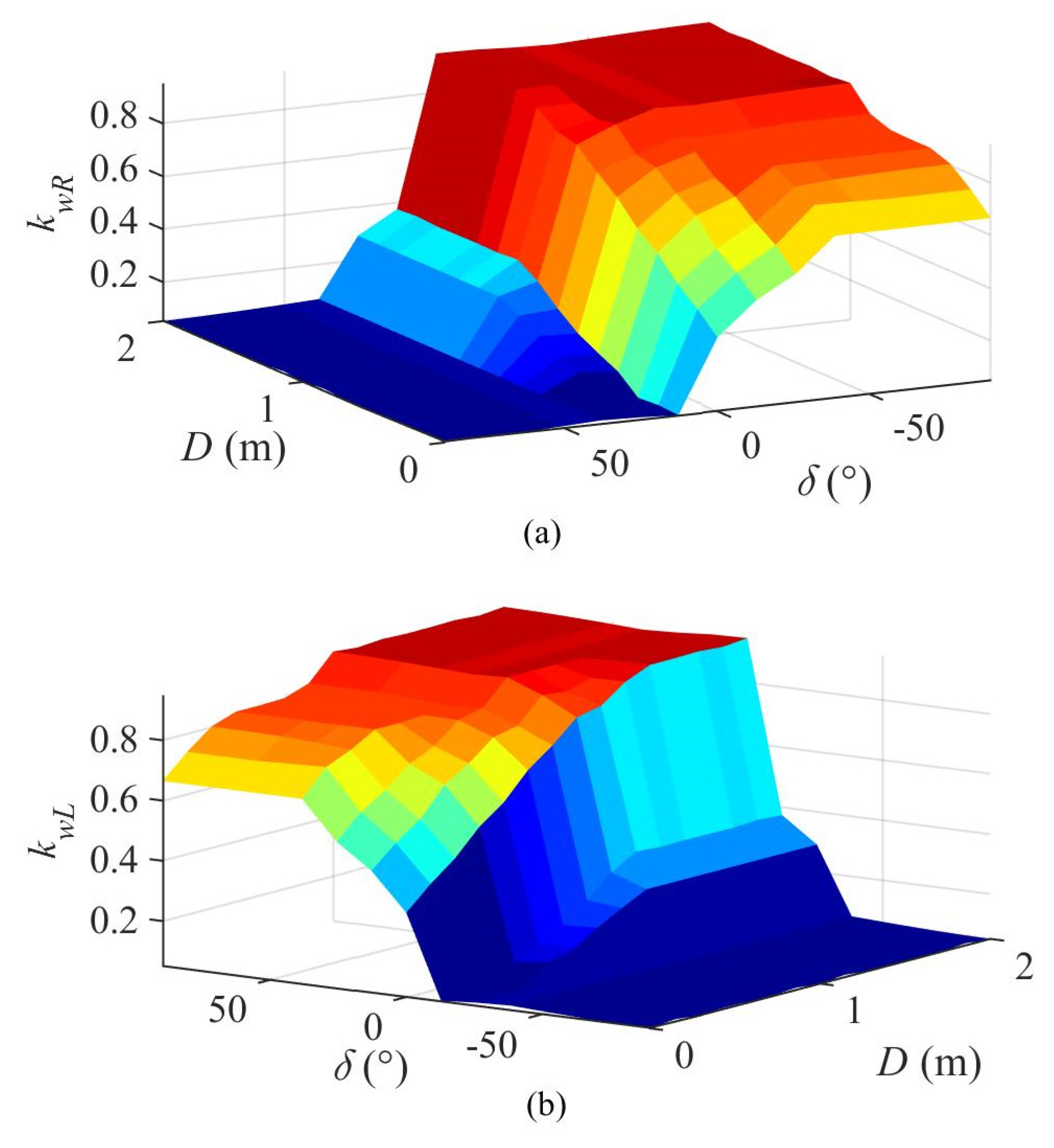
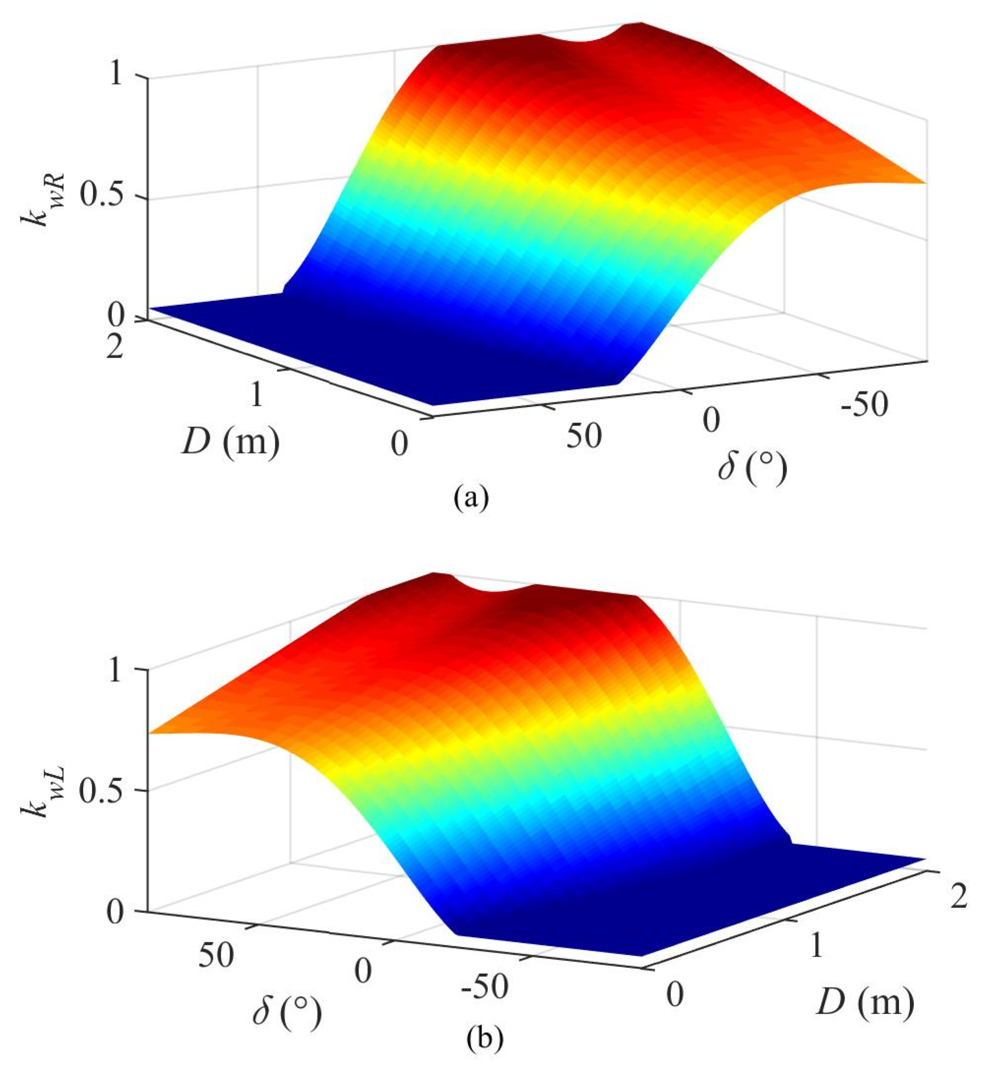
2.3. Approximation of Surfaces

The standard way to describe an area is through a table or through an equation. When the area is approximated through a table, certain values are selected from the area and arranged in a table. This method is simple but ineffective in terms of implementation into the microcontroller due to its limited memory. Therefore, it is much more effective to describe the area with an equation. We can describe the area with an equation in an implicit and explicit shape. An equation in the form F(x, y, z) = 0 is called implicit equation of area if two assumptions are met:

• the coordinates x, y, z from each point Q = [x, y, z] which lies on the area, conform to the equation,
• each Q point on the x, y, z of which Q = [x, y, z] from which the coordinates conform to the equation, represents a point of area [28].

A special case of the equation is an equation in the form z = f(x, y). If this equation is an equation of a specific area, we call it the explicit equation of the area [28]. Equation (9) describes the general form of the explicit equation of surface in polynomial form where x, y is the independent variable area, z is the dependent area variable, p_ij are the coefficients of the polynomial, m is the highest power of x, n is the highest power of y.

$$\begin{array}{l}z={\displaystyle {\displaystyle \sum }_{i=0}^m{\displaystyle \sum }_{j=0}^{n-i}}{p}_{ij}·x^i·y^j\mathrm{if}m\le n\\ z={\displaystyle {\displaystyle \sum }_{j=0}^n{\displaystyle \sum }_{i=0}^{m-j}}{p}_{ij}·x^i·y^j\mathrm{if}m>n\end{array}$$

(9)

If we replace variable x with D, y with δ and create multiples of the maximum speed of the right engine k_wR and left engine k_wL, we get (10).

$$\begin{array}{l}\begin{array}{c}{k}_{wR}={\displaystyle {\displaystyle \sum }_{i=0}^m{\displaystyle \sum }_{j=0}^{n-i}}{p}_{ij}·D^i·{\delta }^j \\ k_{wL}={\displaystyle {\displaystyle \sum }_{i=0}^m{\displaystyle \sum }_{j=0}^{n-i}}{p}_{ij}·D^i·{\delta }^j\end{array}\mathrm{if}m\le n\\ \begin{array}{c}{k}_{wR}={\displaystyle {\displaystyle \sum }_{j=0}^n{\displaystyle \sum }_{i=0}^{m-j}}{p}_{ij}·D^i·{\delta }^j\\ k_{wL}={\displaystyle {\displaystyle \sum }_{j=0}^n{\displaystyle \sum }_{i=0}^{m-j}}{p}_{ij}·D^i·{\delta }^j\end{array}\mathrm{if}m>n\end{array}$$

(10)

The largest influence on control quality of mathematical model has powers m, n, coefficients p_ij and p_i, q_i which are introduced in exponential function approximation method.

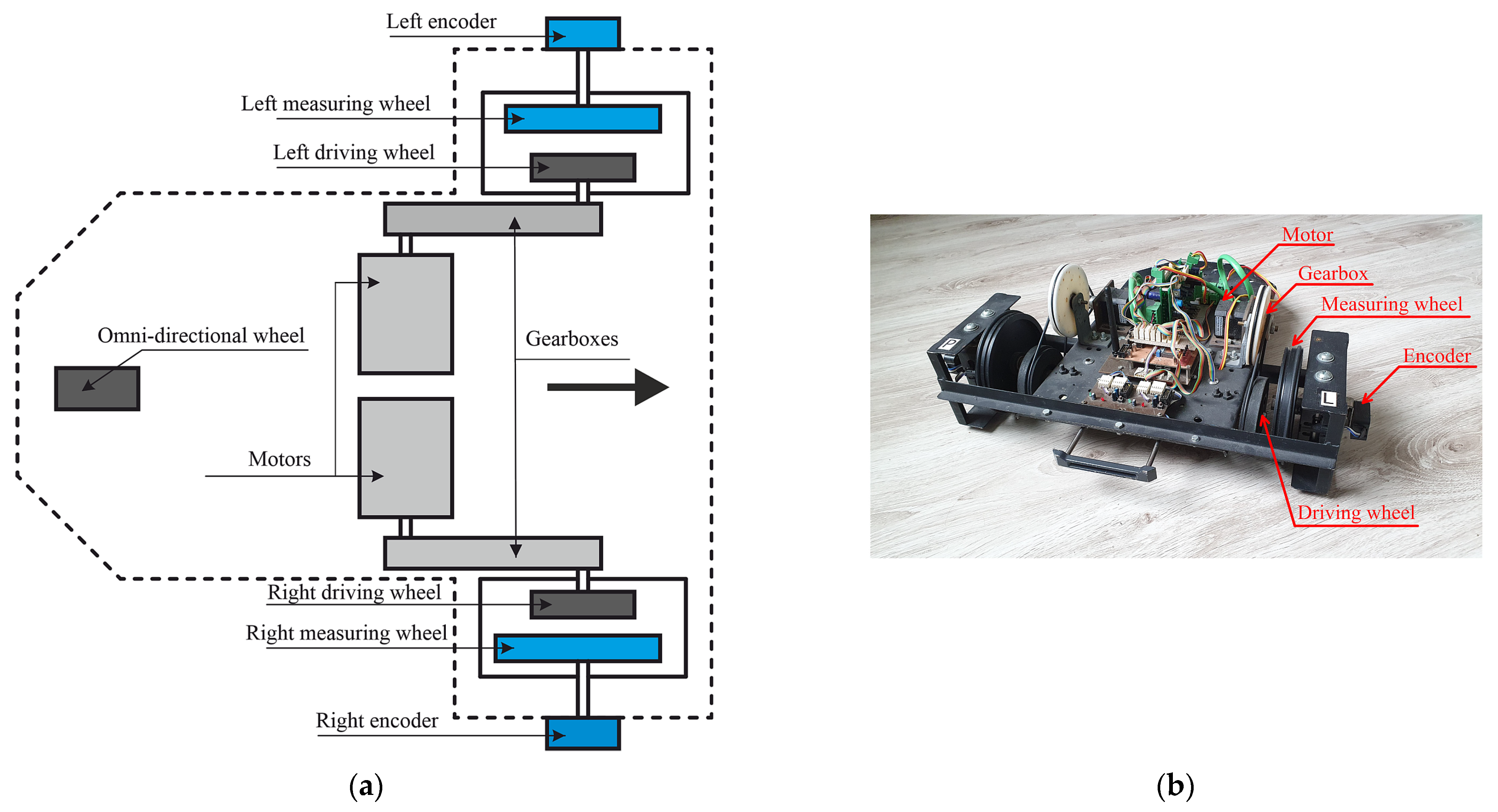
2.4. EN20 Mobile Robot

EN20 mobile robot is based on differential steering chassis and can be operated wirelessly. The principal scheme of this robot is shown in Figure 3. The main parameters of the robot platform are: width = 0.5 m, length = 0.5 m, weight = 4.2 kg, and wheel diameter = 0.1 m.

Communication with the drive modules, incremental sensors, power monitor with control module runs according to the SPI communication standard in a four-wire connection with a data flow rate of 1 Mbps. Data received through SPI. The control unit is based on C8051F340 microcontroller which also secures communication with PC for data transfer. The microcontroller features an on-board USB 2.0 function controller with an integrated transceiver and on-chip clock recovery. It includes a core with 50 MHz performance along with 64 kB Flash, 4.25 kB RAM. On-chip analog features include a 10-bit, 20-ch A-D converter, voltage reference, an internal oscillator, two comparators, and a temperature sensor.

The controller receives information required by fuzzy controller and subsequently calculates control actions for each driving wheel. The mentioned microcontroller combines the communication standards UART and SPI. UART is a device exclusively designated for communication with the control computer via the full-duplex wireless protocol ZigBee. The second type of communication is SPI, where the module is set as “MASTER” in a 4-wire connection with the possibility of connecting eight SPI “SLAVE” modules [29]. Communication with PC is solved through a virtual serial port via USB (controller CP2102). BLY171S 24V-4000 BLDC motors are controlled by dedicated drivers designed specifically for this robot to drive the mobile robot considering effects described in [30]. Velocity measurement of drive wheels of the robot is provided by optical incremental sensors TP 6.35 1024 BZ TTL with a resolution of 1024 pulses per revolution.

3. Results

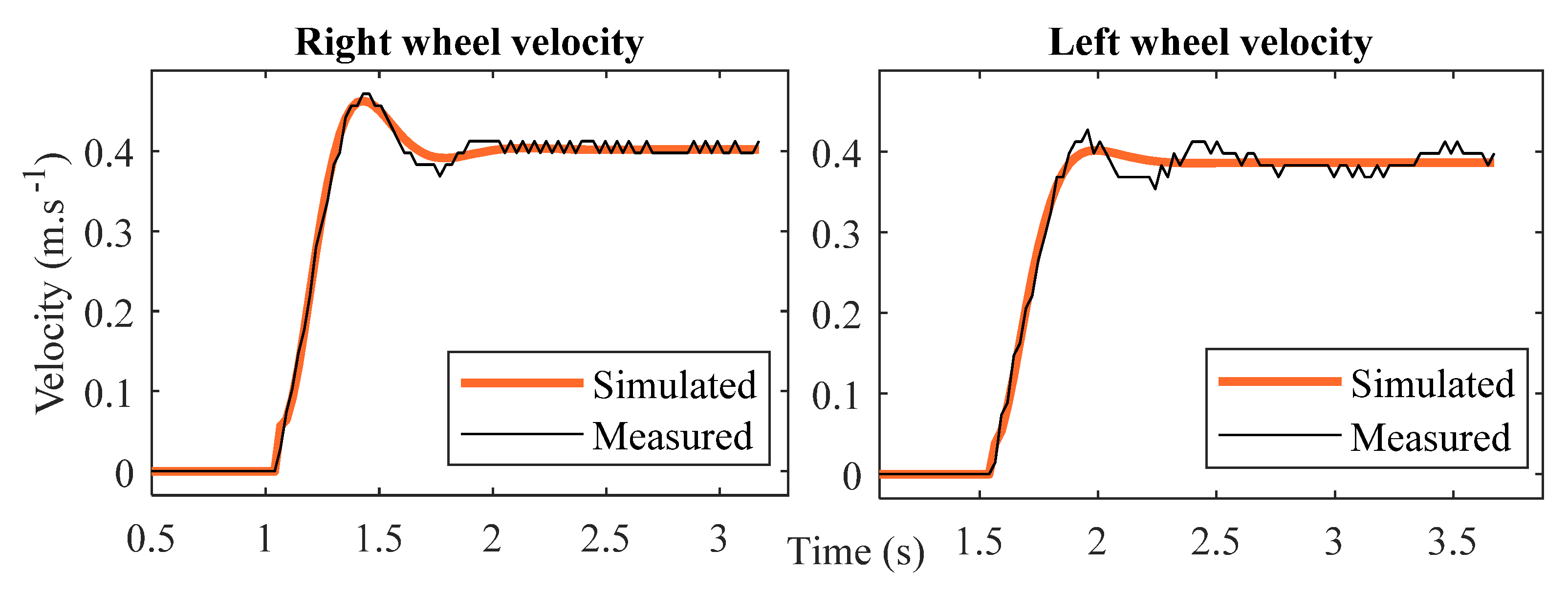
3.1. Identification of EN20 Robot Dynamics

The dynamic model of the robot was obtained from the transfer function of robot’s response on step input signal. The obtained dynamics is compared to the real measurement in Figure 4. The transfer function of EN20 robot (11) we used in all simulations.

$$\begin{gathered} V_R\left(s\right)=e^{-0.05s}\frac{0.001s^2+0.006s+0.6672}{s^2+9.656s+99.63} \\ {V}_L\left(s\right)=e^{-0.05s}\frac{0.00064s^2+0.011s+0.69}{s^2+14.62s+107.2} \end{gathered}$$

(11)

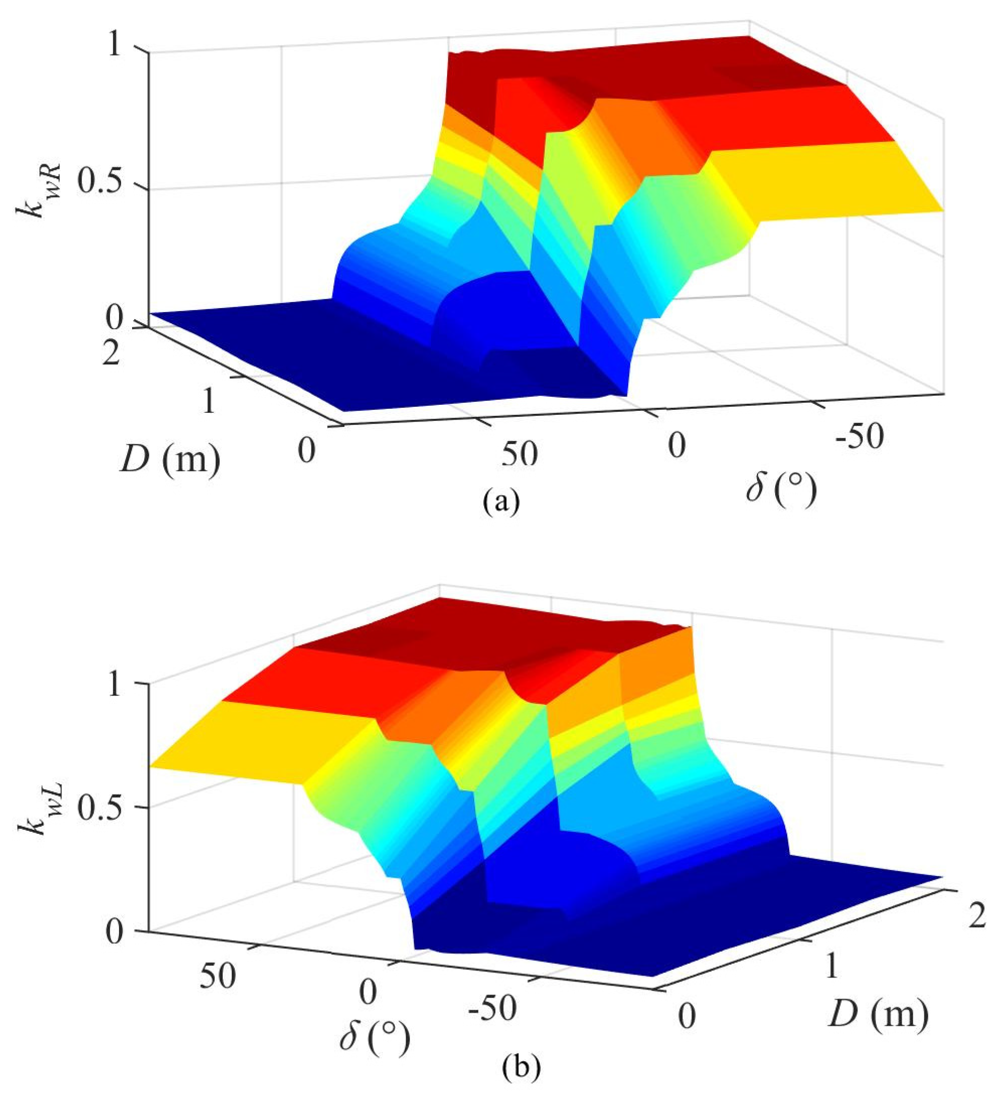
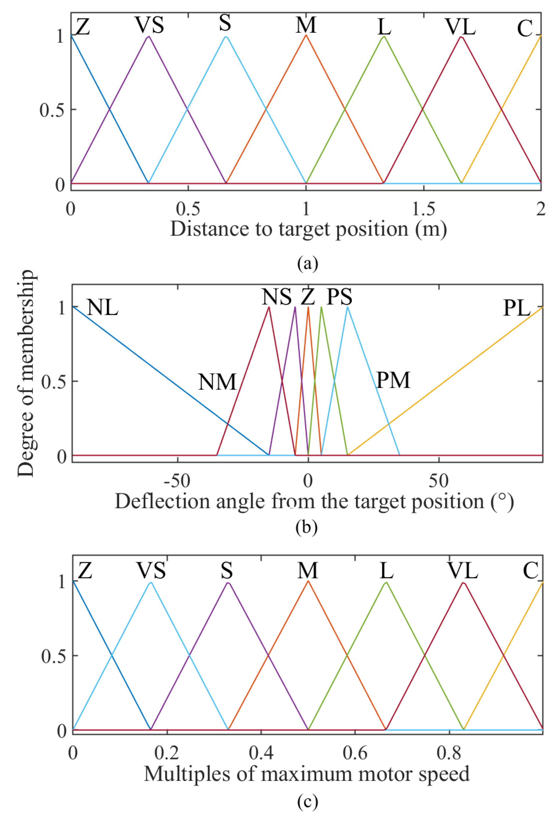
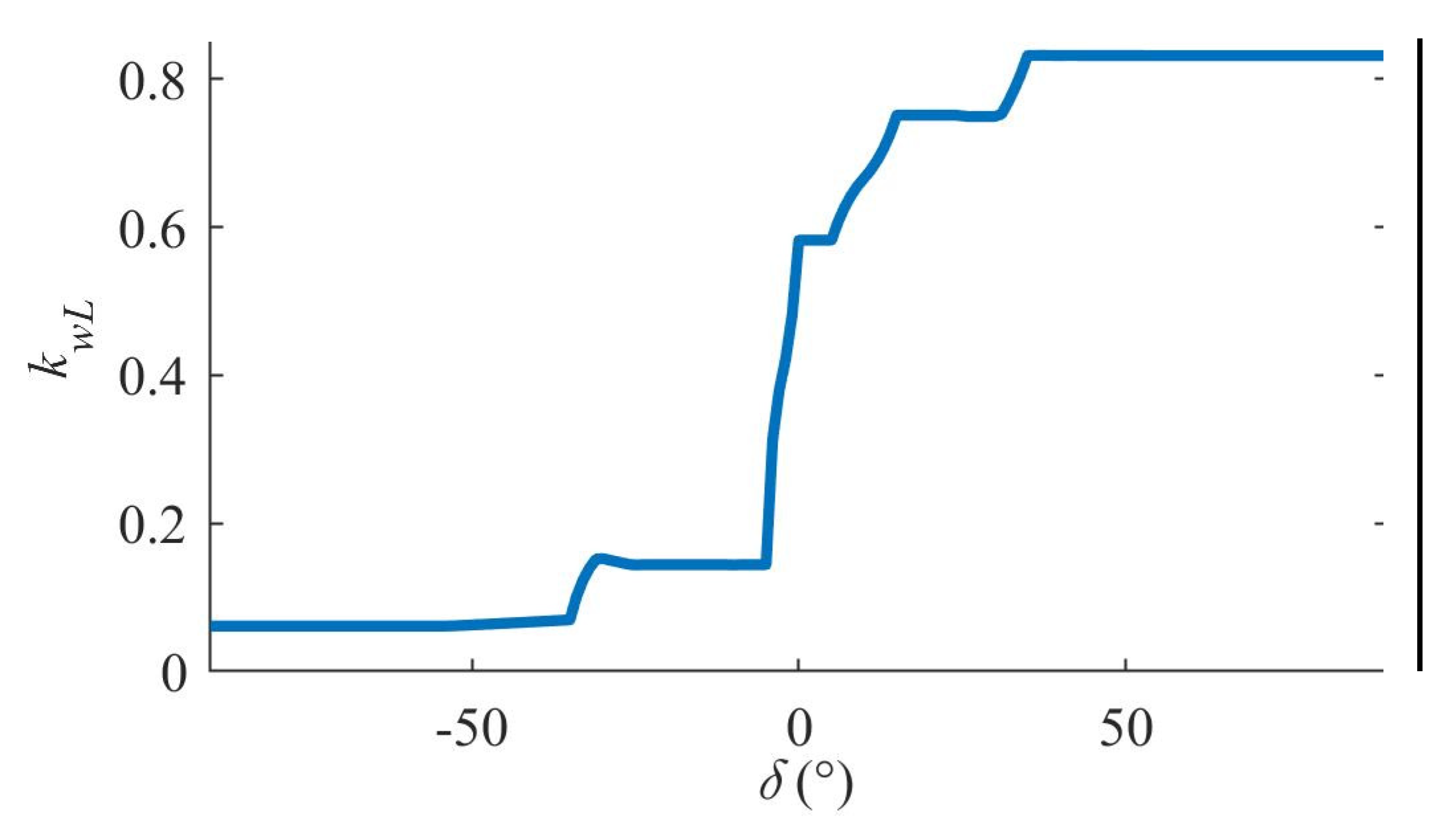
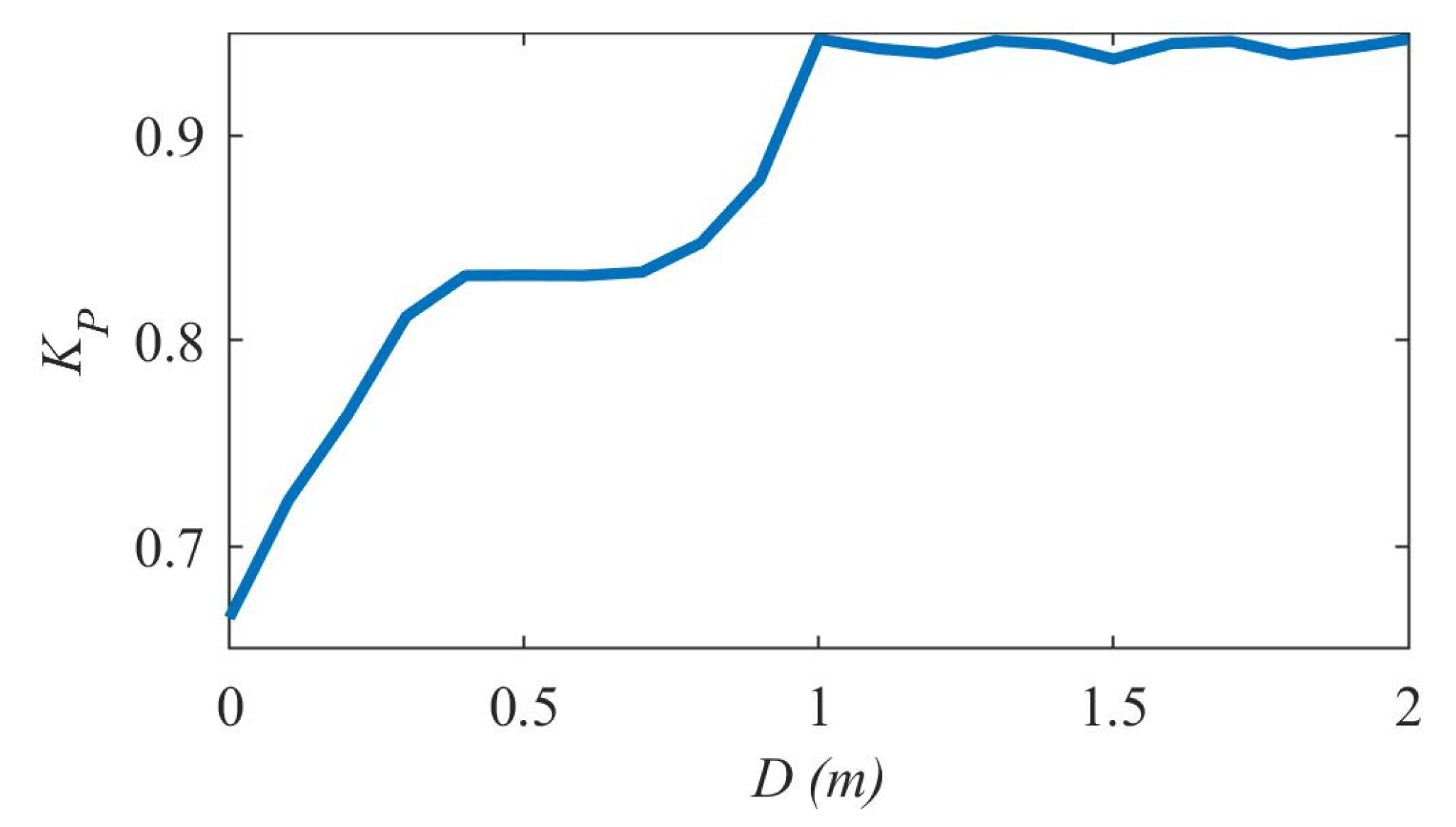
3.2. Fuzzy Controller

As the basis for all approximation methods, we used the control surfaces of the fuzzy controller with 49 inference rules with triangular functions of the respective different linguistic values, as seen in

Table 1. Input and output linguistic values for D, δ, k_wR, and k_wL of fuzzy controller with 49 inference rules.

Distance to Target Position D (m)	Deflection Angle from the Target Position δ (°)	Multiples of Maximum Right and Left Motor Speeds kwR, kwL
Z—zero distance	Z—zero angle	Z—zero multiple
VS—very small distance	PS—positive small angle	VS—very small multiple
S—small distance	PM—positive middle angle	S—small multiple
M—middle distance	PL—positive large angle	M—middle multiple
L—large distance	NS—negative small angle	L—large multiple
VL—very large distance	NM—negative middle angle	VL—very large multiple
C—colossal distance	NL—negative large angle	C—colossal multiple

and their membership functions in Figure 5 with the centroid defuzzification method. This fuzzy controller controls the mobile robot. Inputs to the controller are distance to the target position D and deviation from the target position δ. These output values are calculated based on measurements from the EN20′s right and left incremental sensors. From them, we calculate distances travelled by each wheel since the start. Using the differential chassis kinematics model, we transform these distances to actual robot x, y coordinates and the robot’s angle Θ, and subsequently the inputs to the fuzzy controller from (5), (6) are calculated. Outputs represent multiples (0 to 1) of maximum speed of right k_wR and left motor k_wL. By using 12 V supply voltage, the maximum speed is approximately 2000 rpm.

Values of these controlled variables are fuzzified by triangular functions. When the deflection angle is beyond the range of ±90°, then the fuzzy controller is overridden, and the robot rotates clockwise to get back within the range. The range of ±90° was chosen to reduce number of membership functions for δ to focus more on controller’s precision at smaller angles. If the distance of the robot from the target position is larger than 2 m, the input value is reduced to 2 m. The decision rules are defined as a set of function pertinences for individual terms of the output linguistic variables that must be assigned to a sharp value of the control action within the allowed range [14,31].

The choice of mentioned fuzzy controller parameters was first tested in simulations. The effect of improvement of fuzzy controller control quality decreased with an increasing number of rules as was presented by [15]. The same trend with the increasing number of rules had inference type. With fewer rules, the resulting control surfaces differed more. In terms of membership function types, we compared the four most common shapes. Best results were achieved with triangular shapes, as shown in Figure 6.

Resulting control surfaces of created controller, which are the subject of following approximations, as illustrated in in Figure 7.

3.3. Approximation of Fuzzy Control Surfaces Using a Table

The most important step in this approximation method is to create custom tables with multiples of k_wR and k_wL based on the proposed fuzzy controller. For both tables it is most important to define the step of incrementing the distance of the mobile robot from the target position k_D and the step of incrementing the angle of deflection of the mobile robot from the target position k_δ. Step values affect the number of rows and columns in the table and thus the amount of data that needs to be stored. The number of rows n_r and columns n_s in a table can be calculated using (12):

$$\begin{array}{l}{n}_r=\left(\frac{D_{\max }-D_{\min }}{k_D}\right)+1\\ n_s=\left(\frac{{\delta }_{\max }-{\delta }_{\min }}{k_{\delta }}\right)+1\end{array}$$

(12)

where D_max is the upper bound of mobile robot’s distance from the target position, D_min is the lower bound of mobile robot’s distance from the target position, δ_max is the upper bound of mobile robot’s deflection angle from the target position, and δ_min is the lower bound of mobile robot’s deflection angle from the target position. Another important step is to determine the corresponding table cell through row i and column j of the table where the value of multiples of the maximum motor speed from fuzzy control surfaces is stored using (13), based on the mobile robot’s D and δ values. The function round rounds decimal value of i or j to the nearest integer.

$$\begin{array}{l}i=round\left(\frac{D}{k_D}\right)+1\\ j=round\left(\frac{\delta +90}{k_{\delta }}\right)+1\end{array}$$

(13)

For our purpose we chose D_max = 2, D_min = 0, δ_max = 90, δ_min = −90. From evaluating multiple combinations of k_D and k_δ we picked, based on both control quality and memory occupancy of tables for each motor, values k_D = 0.5 m and k_δ = 1°. The resulting surfaces of multiples of the maximum speed of the right and the left motor which approximate the fuzzy control surfaces from Figure 7 are shown in Figure 8.

3.4. Approximation of Fuzzy Control Surfaces through a Polynomial

When approximating fuzzy control surfaces via polynomial, we proceed from (10). Polynomials were obtained using surface fitting function in Matlab software. From testing multiple combinations of m and n values, we found that the best average control time is achieved by approximating the fuzzy control surfaces by polynomial with power of m = 1 and n = 5. However, in terms of average absolute and quadratic error area, the optimal approximation is by polynomial with power of m = 5 and n = 5. We inclined to approximate the control surfaces by means of a polynomial with powers m = 1 and n = 5 in (14) because of the smaller average control time, which will ensure that the mathematical model of the mobile robot reaches its destination earlier.

$$\begin{array}{l}{k}_{w_P}=0.3414+0.2346·D-0.01424·\delta -0.0009284·D·\delta \\ -3.348·{10}^{-5}·{\delta }^2-9.647·{10}^{-5}·D·{\delta }^2+3.139·{10}^{-6}·{\delta }^3\\ -4.104·{10}^{-7}·D·{\delta }^3+3.593·{10}^{-8}·{\delta }^4\\ +5.135·{10}^{-9}·D·{\delta }^4+1.159·{10}^{-10}·{\delta }^5\\ k_{w_L}=0.3414+0.2346·D+0.01424·\delta +0.0009284·D·\delta \\ -3.348·{10}^{-5}·{\delta }^2-9.647·{10}^{-5}·D·{\delta }^2-3.139·{10}^{-6}·{\delta }^3\\ +4.104·{10}^{-7}·D·{\delta }^3+3.593·{10}^{-8}·{\delta }^4+5.135·{10}^{-9}·D·{\delta }^4\\ -1.159·{10}^{-10}·{\delta }^5\end{array}$$

(14)

Graphical representation of the polynomials from (14) is shown in Figure 9.

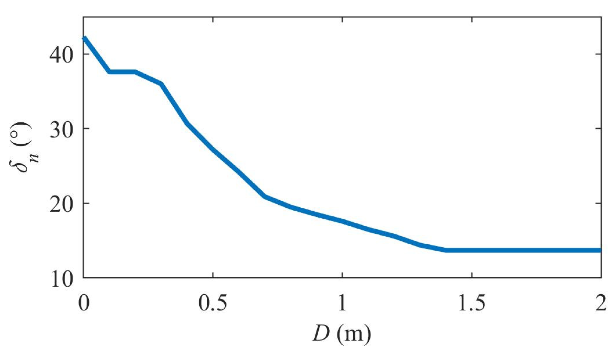
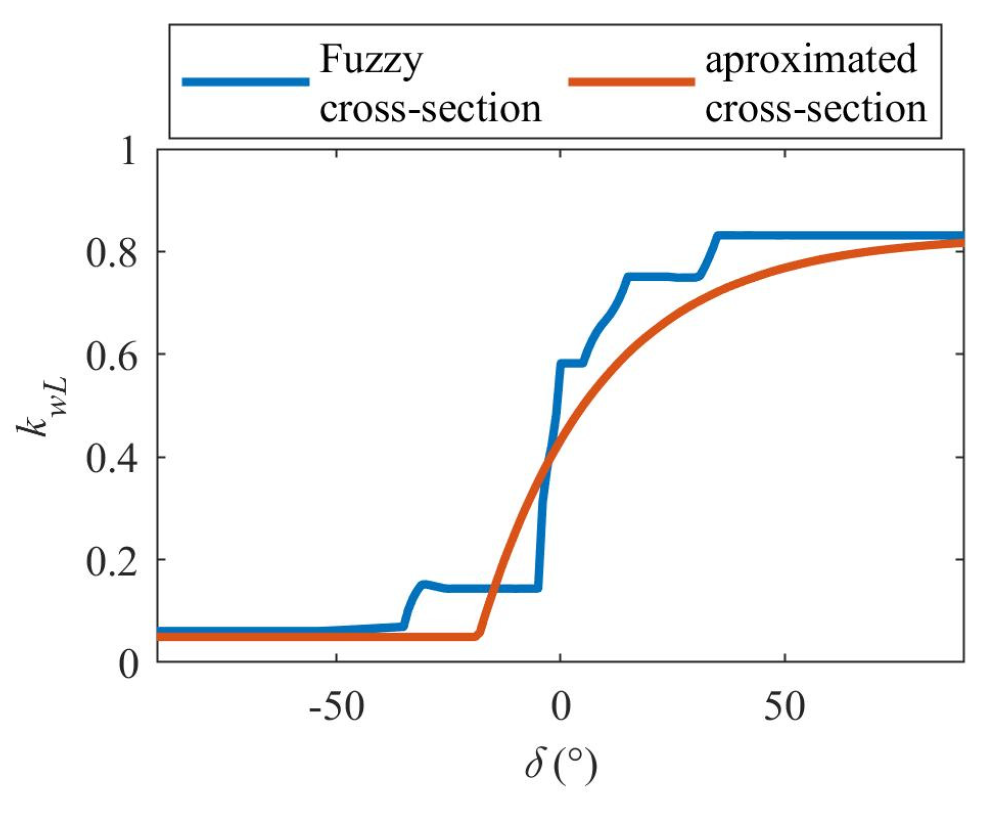
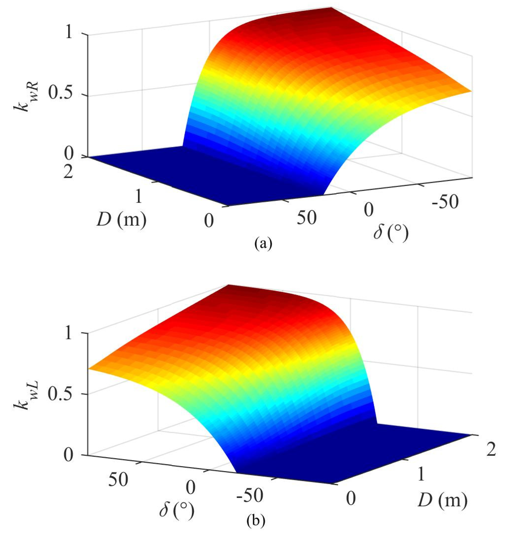
3.5. Approximation of Fuzzy Control Surfaces through Exponential Function

After closer analysis of the fuzzy control surfaces, we noticed that in a cross-section along the δ axis, the dependence of multiples of the maximum motor speed on δ resembles a transfer function of first order system (Figure 10).

In time domain it is defined by function (15) [32].

$$y\left(t\right)=\{\begin{array}{c}0\\ K\left(1-e^{-\frac{t-D}{T}}\right)\end{array}\begin{array}{cc}& t<D\\ & t\ge D\end{array}$$

(15)

where y(t) is function output, K is gain, T is time constant, and D is time delay. The dependence in Figure 10 with use of (15) can be approximated by a derived exponential function (16). Argument of the transfer function is now angle of deflection δ, T is replaced with rise angle δ_n, D is replaced with angle of displacement δ₀, and K is replaced with steady-state value of the cross-section course K_P. Since the control surfaces of the fuzzy controller are symmetrical, in determining the exponential equations, we picked the control surface of the left motor.

$$k_{w_L}=K_P\left(1-e^{\left(-\frac{\delta -{\delta }_0}{{\delta }_n}\right)}\right)$$

(16)

The imperfection of this approximation is that for various fuzzy control area cross-sections along the D axis, we receive different steady-state values K_P and the values of δ_n as shown in Figure 7. In our case values of K_P are values of k_wL at the minimum angle with course shown in Figure 11.

Values of δ₀ and δ_n were used as free parameters in fitting procedure carried out by Matlab’s curve fitting functions. We fitted the fuzzy control areas cross-section with (16) in 0.1 m steps of D. The course of obtained δ_n values is shown in Figure 11. Values of δ₀ were uneven and difficult to describe with an equation course over D so we simplified their calculation by setting them constant δ₀ = −20°. With this value we achieved best correlation between original fuzzy surface and the exponential function approximation.

When the courses of K_P (Figure 11) and δ_n (Figure 12) are approximated by a polynomial, we get (17):

$$k_{w_L}=\left({\displaystyle {\displaystyle \sum }_{i=0}^m}{p}_i·D^i\right)·\left(1-e^{\left(-\frac{\delta -{\delta }_0}{{\displaystyle {{\displaystyle \sum }}_{i=0}^n}{q}_i·D^i}\right)}\right)$$

(17)

where p_i, q_i are the coefficients of polynomials, m is the highest power of the distance of the mobile robot for approximation of K_P, n is the highest power of the distance of the mobile robot for approximation of δ_n. For example, to fit the cross-section of fuzzy control surface in Figure 8 using (16), we got the following values of the parameters: K_P = 0.8318, δ_n = 27.2°, δ₀ = −20°. Approximated exponential function together with original fuzzy controller course is shown in Figure 13.

We fitted courses in Figure 11 and Figure 12 in the same way. We tested obtained approximation functions for various combinations of powers m and n and substituted them into (17). Focus was on minimalizing average control areas. In this respect, we chose approximation of the steady-state K_P value with a first-order polynomial and approximation of rise angle δ_n with the sixth order polynomial. Equation (18) represents the final form of exponential function equations for both motors.

$$\begin{array}{l}{k}_{w_L}=\left(\begin{array}{l}0.754\\ +0.1218·D\end{array}\right)·\left(1-e^{\left(-\frac{\delta +20}{\begin{array}{l}38.84-6.524·D-76.18·D^2\\ +127.4·D^3-93.27·D^4+33.38·D^5\\ -4.699·D^6\end{array}}\right)}\right)\\ k_{w_P}=\left(\begin{array}{l}0.754\\ +0.1218·D\end{array}\right)·\left(1-e^{\left(-\frac{-\delta +20}{\begin{array}{l}38.84-6.524·D-76.18·D^2\\ +127.4·D^3-93.27·D^4+33.38·D^5\\ -4.699·D^6\end{array}}\right)}\right)\end{array}$$

(18)

Figure 14 shows the resulting control surfaces approximation of the fuzzy control surfaces using an exponential function.

Comparison of the control time, absolute, and quadratic control area values for each fuzzy control area approximation method is shown in

Table 2. Impact of fuzzy control surface approximation methods on the control quality of the mathematical model of the mobile robot EN20.

Control Method	Control Time treg (s)	Absolute Error Control Area IAE	Squared Error Control Area ISE
Fuzzy with 49 inference rules	40.032	3.329	0.529
Table with kD = 0.5 m and kδ = 1°	40.113	3.392	0.538
Polynomial with m = 1 and n = 5	42.482	5.107	0.982
Exponential function with m = 1, n = 6 and δ0 = −20°	43.216	3.651	0.537

.

Differences between fuzzy control surface approximation methods can also be shown on the paths of the mobile robot simulation from the beginning of the coordinate system to the target point, which is at distance of 10 m in Figure 15.

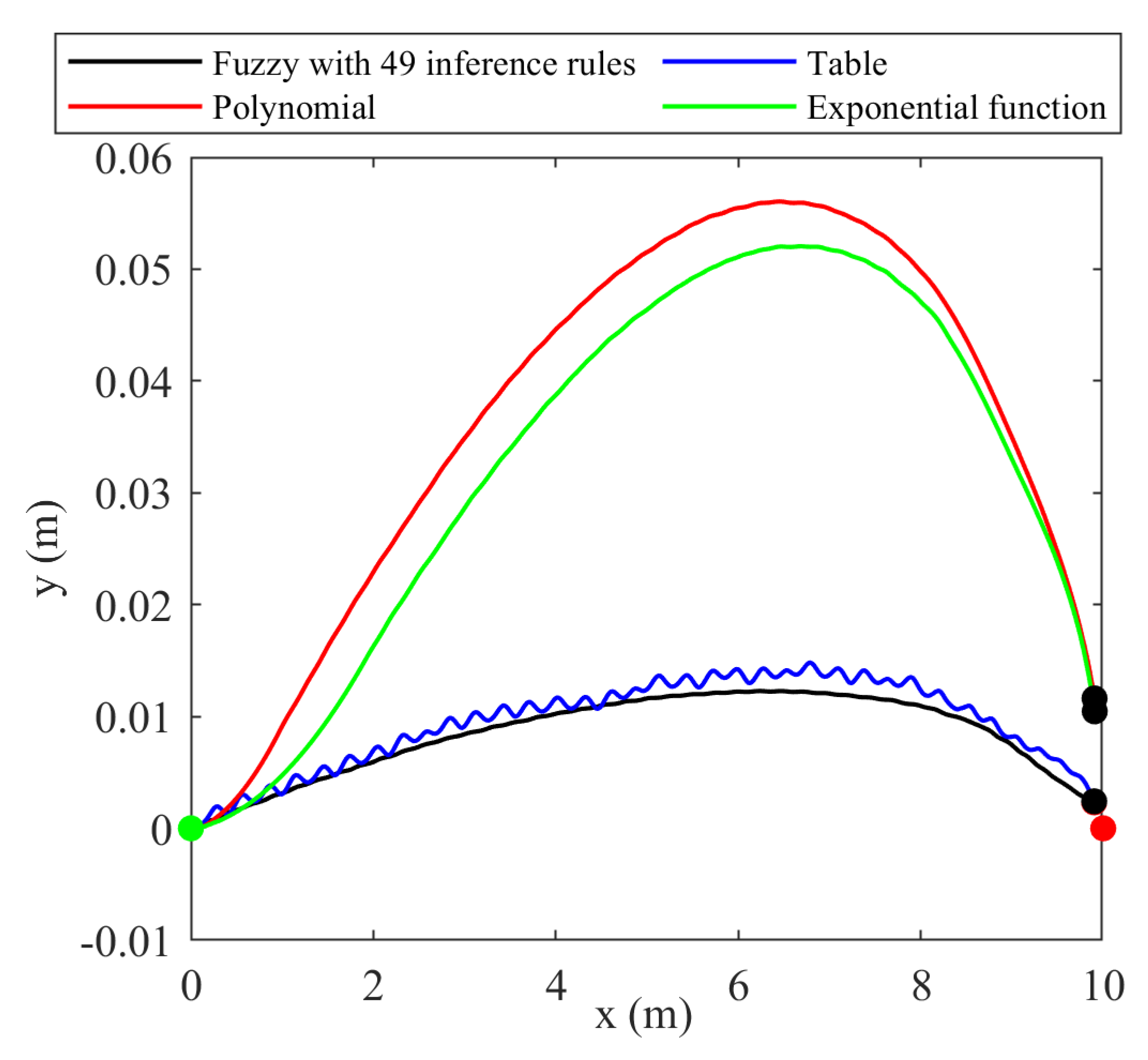
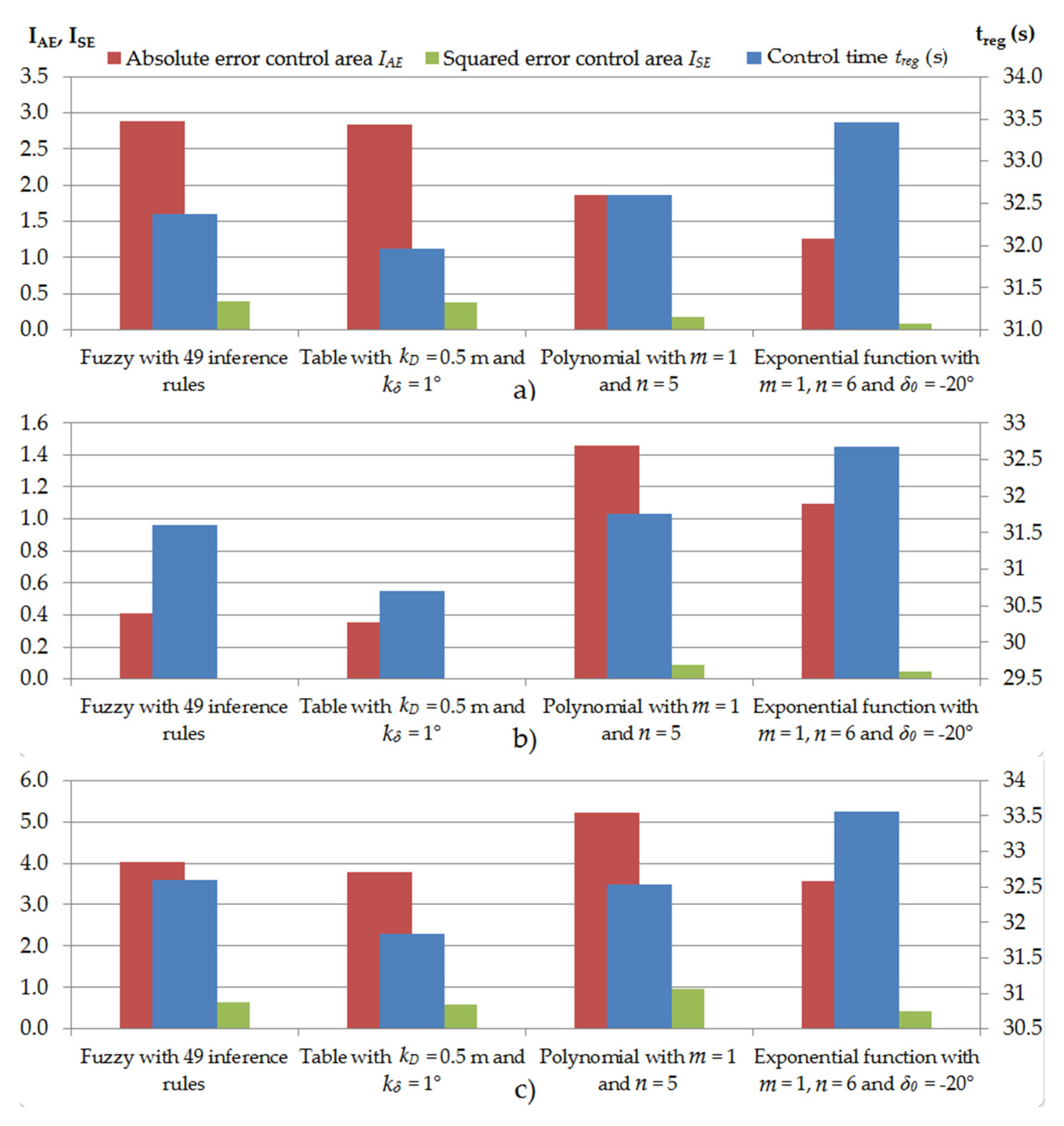
3.6. Real-World Testing

The main parameter influencing the control time is the maximum speed of the right and left engine of the mobile robot. Therefore, when analyzing the impact of the fuzzy control surface method on the control quality of the EN20 mobile robot in real-world conditions, we set the maximum speed of both motors to 60%. The reason for limiting motor speeds to 60% is due to the robot’s current limiter activation at acceleration to higher speeds to reduce the current supplied to the motor drives, thus reducing motors speed [6]. Because of this fact, the used identified mathematical model of the robot is relevant only up to 60% of maximum speed. After implementing approximated controllers, we have made several measurements of the travelled paths of the EN20 mobile robot using different methods of approximation of fuzzy control surfaces. Measurements of the EN20 mobile robot path under real conditions for all the proposed control methods were made on a straight track of 10 m in length and with an initial angle of deflection of the mobile robot from the target position of 0°, 90°, and −90°. Sample time for receiving data was chosen 0.1 s. Obtained average control quality parameters for each control method based on 10 measurements are given in Figure 16. For evaluating the control quality, we focused on three quantitative indicators: control time t_reg, absolute (I_AE), and the quadratic (I_SE) control error area stated in (7), (8). Calculated control criterions had in all tests of polynomial and exponential approximations deviation of ± 5%. With table approximation in some measurements the robot turned more abruptly, which caused greater deviations of ± 8% from the average.

We also compared the measured paths of the mobile robot for each control method and with the initial angle of deflection of the mobile robot from the target position of 0°, 90°, and −90° graphically in Figure 17.

In Figure 17 there is the present oscillation in control with all methods. Oscillations during real experiments were negligible but, in the figure, they are accentuated by scaling of the y-axis. The main reason for their presence is slightly different gear ratios of right and left gearboxes and measurement errors of the robot’s position. From the real testing comparison, the approximation by the table is the most accurate from all approximations to the original fuzzy controller and the fastest method among all compared. The control time advantage over the original fuzzy controller is due to quicker execution times of the table approximation method and made the table controller better in the real tests. Approximations by polynomial and exponential functions showed different robot trajectory courses than the previous two. This was due to the smoother shape of approximated control surfaces by (14) and (18). After the start robot changed its direction more gradually which led to longer control times and larger control error areas. The benefit of this is that oscillations in trajectory are less distinct for these two methods.

To clearly show the effect of the approximations on reducing computational demand on the processor, we measured the average computation time of fuzzy output for 100 samples during real-world tests. The obtained values along with memory and RAM occupation are in

Table 3. Comparison of computation load of C8051F340 microcontroller with fuzzy controller and approximation methods.

Parameter	Fuzzy Controller	Table Approximation	Polynomial Approximation	Exponential Function Approximation
Average computation time (ms)	1224.4	0.033	1.992	2.490
Memory occupation (%)	4	8	2	2
RAM occupation (%)	18	4	2	2

.

4. Discussion

Verification of presented approximation methods was demonstrated on the fuzzy controller with 49 interference rules. The number of rules directly affects the shape of control surfaces. In general, with fewer rules, the created control surface becomes more broken. Given that, approximations by polynomial and exponential function can become less precise due to their continuous shapes. On the other hand, approximation by the table is more adaptive to the fuzzy control surface shape. In cases when fewer rules are sufficient or the control surface is sharper, this method is more universal. We tested all the methods of approximation of fuzzy control surfaces in real conditions with the EN20 mobile robot. Although approximations through polynomial and exponential function are less precise, they are much more appropriate in terms of microcontroller implementation. By comparing these two methods of approximation, we found that polynomial approximation had a shorter control time, while the exponential approximation had smaller control error areas. The robustness of the approximated fuzzy controllers is conditioned by the accuracy of the approximation to the original fuzzy controller in a defined range of input variables. Due to the algebraic form of the functions, preventing the loss of control stability so that the input variables do not get outside their defined range in which the outputs are approximated must be programmatically solved by the conditions: If input < input_min then input = input_min and vice versa. Another kind of possible loss of robustness could be in extreme cases of the approximation functions when a value of any term of the function would overflow and caused wrong output value.

These approximation methods can easily be implemented into different types of microcontrollers by being represented by algebraic equations. Another advantage of the presented approximation methods is a less demanding source code, which reduces memory requirements, and the execution time of the program is still very fast. The direction of research in this area should focus both on the search for further approximation methods, simplifying the acquisition of approximations and on the investigation of the control response of these methods.

5. Conclusions

In this paper, we presented the new possibilities of approximation of fuzzy control surfaces into the microcontrollers without high requirements on microcontroller memory. We compared the existing way of approximating control surfaces through a table and two proposed approximations through a polynomial and exponential function with a regular fuzzy controller. Approximation through the table is simple and accurate, but inefficient due to its higher demand on memory for storing all table values. For this reason, the novelty of the paper is in using approximation methods defined by polynomial and exponential functions. The theoretical and practical functionality of the approximations was tested on the task of navigating the EN20 mobile robot to the target position. Real-world test results verified the functionality of simulations and showed usability and suitability of the approximation methods for implementation into a microcontroller. From the comparison of simulated and experimental results, it can be seen that the simulated model of the EN20 mobile robot described the real robot’s performance accurately enough.

Compared to previously presented works, the main benefit is the replacement of a complex calculation of fuzzy control by algebraic equations for the direct calculation of corresponding output values of the fuzzy controller. Compared to the table approximation method the memory required to store the controller with polynomial and exponential function is reduced. Another benefit is the simplicity of implementation into microcontrollers. Instead of defining all membership functions and fuzzy rules or assigning all table values, the approximated fuzzy controller is in form of two equations using standard mathematical operations.

References

1. Rubio, F.; Valero, F.; Llopis-Albert, C. A review of mobile robots: Concepts, methods, theoretical framework, and applications. Int. J. Adv. Robot. Syst. 2019, 16, 1–22. [Google Scholar] [CrossRef] [Green Version]
2. Zadeh, L.A. From computing with numbers to computing with words: From manipulation of measurements to manipulation of perceptions. In The Dynamics of Judicial Proof; MacCrimmon, M., Tillers, P., Eds.; Physica: Heidelberg, Germany, 2002; Volume 94, pp. 81–117. [Google Scholar] [CrossRef]
3. Omrane, H.; Masmoudi, M.S.; Masmoudi, M. Fuzzy Logic Based Control for Autonomous Mobile Robot Navigation. Comp. Int. Neurosci. 2016, 2016, 9548482. [Google Scholar] [CrossRef] [PubMed] [Green Version]
4. Castillo, O. Interval Type-2 Mamdani Fuzzy Systems for Intelligent Control. In Combining Experimentation and Theory Studies in Fuzziness and Soft Computing; Trillas, E., Bonissone, P., Magdalena, L., Kacprzyk, J., Eds.; Springer: Berlin, Germany, 2012; pp. 163–177. [Google Scholar] [CrossRef]
5. Masmoudi, M.S.; Krichen, N.; Masmoudi, M.; Derbel, N. Fuzzy logic controllers design for omnidirectional mobile robot navigation. Appl. Soft Comput. 2016, 49, 901–919. [Google Scholar] [CrossRef]
6. Bai, Z.; Lu, Y.; Li, Y. Method of Improving Lateral Stability by Using Additional Yaw Moment of Semi-Trailer. Energies 2020, 13, 6317. [Google Scholar] [CrossRef]
7. Urrea, C.; Páez, F. Designand Comparison of Strategies for Level Control in a Nonlinear Tank. Processes 2021, 9, 735. [Google Scholar] [CrossRef]
8. García-Sánchez, J.R.; Tavera-Mosqueda, S.; Silva-Ortigoza, R.; Hernández-Guzmán, V.M.; Marciano-Melchor, M.; Rubio, J.d.J.; Ponce-Silva, M.; Hernández-Bolaños, M.; Martínez-Martínez, J. A Novel Dynamic Three-Level Tracking Controller for Mobile Robots Considering Actuators and Power Stage Subsystems: Experimental Assessment. Sensors 2020, 20, 4959. [Google Scholar] [CrossRef]
9. García-Sánchez, J.R.; Tavera-Mosqueda, S.; Silva-Ortigoza, R.; Hernández-Guzmán, V.M.; Sandoval-Gutiérrez, J.; Marcelino-Aranda, M.; Taud, H.; Marciano-Melchor, M. Robust Switched Tracking Control for Wheeled Mobile Robots Considering the Actuators and Drivers. Sensors 2018, 18, 4316. [Google Scholar] [CrossRef] [Green Version]
10. Serrano, M.E.; Scaglia, G.J.E.; Rómoli, S.; Mut, V.; Godoy, S. Trajectory tracking controller based on numerical approximation under control actions constraints. In Proceedings of the 2014 IEEE Biennial Congress of Argentina (ARGENCON), San Carlos de Bariloche, Argentina, 11–13 June 2014; pp. 37–42. [Google Scholar] [CrossRef]
11. Serrano, M.E.; Godoy, S.A.; Rómoli, S.; Scaglia, G.J.E. A Numerical Approximation-Based Controller for Mobile Robots with Velocity Limitation. Asian J. Control 2017, 19, 2165–2177. [Google Scholar] [CrossRef]
12. Oltean, S.E.; Dulău, M.; Puskas, R. Position control of Robotino mobile robot using fuzzy logic. In Proceedings of the IEEE International Conference on Automation, Quality and Testing, Robotics (AQTR), Cluj-Napoca, Romania, 28–30 May 2010. [Google Scholar] [CrossRef]
13. Faisal, M.; Hedjar, R.; Sulaiman, M.A.; Al-Mutib, K. Fuzzy Logic Navigation and Obstacle Avoidance by a Mobile Robot in an Unknown Dynamic Environment. Int. J. Adv. Rob. Syst. 2013, 10, 37. [Google Scholar] [CrossRef]
14. Štefek, A.; Pham, V.T.; Krivanek, V.; Pham, K.L. Optimization of Fuzzy Logic Controller Used for a Differential Drive Wheeled Mobile Robot. Appl. Sci. 2021, 11, 6023. [Google Scholar] [CrossRef]
15. Kósa, P.; Olejár, M.; Palková, Z.; Hrubý, D.; Cviklovič, V.; Harničárová, M.; Valícek, J. The effect of the number of inference rules of a fuzzy controller on the quality of control of a mobile robot. MATEC Web Conf. 2019, 299, 05002. [Google Scholar] [CrossRef] [Green Version]
16. Abdalla, M.; Al-Jarrah, T. Optimal Fuzzy Controller: Rule Base Optimizer Generation. Jrn. Contr. Eng. Appl. Inf. 2018, 20, 76–86. [Google Scholar]
17. Muniz, L.; Carmo, M.; Santos, M.; Santos, A.; Mercorelli, P. Case Study: Aspects of Fuzzy Controller Implementation in Embedded Systems. In Proceedings of the International Conference on Mathematics and Computers in Science and Engineering (MACISE), Madrid, Spain, 18–20 January 2020; pp. 155–158. [Google Scholar] [CrossRef]
18. Purwanto, F.H.; Utami, E.; Pramono, E. Implementation and Optimization of Server Room Temperature and Humidity Control System using Fuzzy Logic Based on Microcontroller. J. Phys. Conf. Ser. 2018, 1140, 012050. [Google Scholar] [CrossRef]
19. Ridwan, M.; Taryo, T. Implementation of Fuzzy Logic Controller for Pressure Sensor Calibration Chamber. Int. J. Automot. Mech. Eng. 2021, 18, 8825–8832. [Google Scholar] [CrossRef]
20. Uzunovic, T.; Turkovic, I. Implementation of microcontroller based fuzzy controller. In Proceedings of the 6th IEEE International Conference Intelligent Systems, Sofia, Bulgaria, 6–8 September 2012; pp. 310–315. [Google Scholar] [CrossRef]
21. Carvajal, O.; Castillo, O. Implementation of a Fuzzy Controller for an Autonomous Mobile Robot in the PIC18F4550 Microcontroller. In Hybrid Intelligent Systems in Control, Pattern Recognition and Medicine; Springer: Cham, Switzerland, 2020; Volume 827, pp. 315–325. [Google Scholar] [CrossRef]
22. Abood, M.S.; Thajeel, I.K.; Alsaedi, E.M.; Hamdi, M.M.; Mustafa, A.S.; Rashid, S.A. Fuzzy Logic Controller to control the position of a mobile robot that follows a track on the floor. In Proceedings of the 4th International Symposium on Multidisciplinary Studies and Innovative Technologies (ISMSIT), Istanbul, Turkey, 22–24 October 2020; pp. 1–7. [Google Scholar] [CrossRef]
23. Olejár, M.; Hrubý, D.; Lukáč, O. Methods of Control of Microclimatic Conditions in Enclosed Spaces and Their Influence on Electricity Saving, 1st ed.; Slovak University of Agriculture in Nitra: Nitra-Chrenová, Slovakia, 2009; pp. 74–141. (In Slovak) [Google Scholar]
24. Sekaj, I. Fuzzy Logic Controllers and Their Replacement by a Non-Fuzzy Approximation Algorithm. IFAC Proc. Vol. 1997, 30, 363–368. [Google Scholar] [CrossRef]
25. Dombi, J.; Hussain, A. A new approach to fuzzy control using the distending function. J. Process. Control 2020, 86, 16–29. [Google Scholar] [CrossRef]
26. Peri, V. Fuzzy Logic Controller for an Autonomous Mobile Robot. Master’s Thesis, Cleveland State University, Cleveland, OH, USA, 2005. Available online: https://academic.csuohio.edu/embedded/Publications/Thesis/Mohan%20Thesis.pdf (accessed on 21 April 2021).
27. Vacho, L.; Olejár, M.; Hrubý, D.; Cviklovič, V.; Valíček, J.; Palková, Z.; Harničárová, M.; Tozan, H. Identification of Dynamics of Movement of the Differential Mobile Robotic Platform Controlled by Fuzzy Controller. Teh. Vjesn. 2019, 26, 1642–1649. [Google Scholar] [CrossRef]
28. Holmes, M.H. Introduction to the Foundations of Applied Mathematics, 1st ed.; Springer: New York, NY, USA, 2009; pp. 205–264. [Google Scholar]
29. Cviklovič, V.; Olejár, M.; Hrubý, D.; Lukáč, O. Odometry in Navigation of Autonomous Mobile Robots, 1st ed.; SUA: Nitra, Slovakia, 2013; pp. 30–68. [Google Scholar]
30. Zajkowski, K.; Rusica, I.; Palkova, Z. The use of CPC theory for energy description of two nonlinear receivers. In Proceedings of the 22nd International Conference on Innovative Manufacturing Engineering and Energy (IManE&E), Chisinau, Moldova, 31 May–2 June 2018. [Google Scholar] [CrossRef]
31. Caraveo, C.; Valdez, F.; Castillo, O. A New Meta-Heuristics of Optimization with Dynamic Adaptation of Parameters Using Type-2 Fuzzy Logic for Trajectory Control of a Mobile Robot. Algorithms 2017, 10, 85. [Google Scholar] [CrossRef] [Green Version]
32. Mikleš, J.; Fikar, M. Process Modelling, Identification, and Control, 1st ed.; Springer: Berlin/Heidelberg, Germany, 2007; pp. 221–251. [Google Scholar]
Figure 1. Principal scheme of differential chassis.
Processes 09 01602 g001
Figure 2. Meaning of input quantities to EN20 mobile robot fuzzy controller.
Processes 09 01602 g002
Figure 3. (a) EN20 mobile robot chassis scheme; (b) picture of the EN20 robot platform.
Processes 09 01602 g003
Figure 4. Comparison of measured and simulated velocities of right and left wheel.
Processes 09 01602 g004
Figure 5. Membership functions of linguistic variables for mobile robot’s: (a) distance D from target position; (b) deviation δ from target position; (c) multiples of maximum speed of right kwR and left kwL motor.
Processes 09 01602 g005
Figure 6. Effect of membership functions type on control criterions.
Processes 09 01602 g006
Figure 7. Fuzzy controller surfaces with 49 inference rules for multiples of maximum speed of: (a) right engine kwR; (b) left engine kwL.
Processes 09 01602 g007
Figure 8. Surfaces for multiples of the maximum speed: (a) of the right engine; (b) of the left engine which are the approximation of the fuzzy control surfaces by a table with kD = 0.5 m and kδ = 1°.
Processes 09 01602 g008
Figure 9. Fuzzy control surfaces of the maximum speed: (a) of the right engine; (b) of the left engine approximated by means of a polynomial with power m = 1 and n = 5.
Processes 09 01602 g009
Figure 10. Cross-section of multiples of the maximum speed of the left engine along δ axis and at the distance of the mobile robot from the target position D = 0.5 m.
Processes 09 01602 g010
Figure 11. Steady-state value KP course.
Processes 09 01602 g011
Figure 12. Rise angle δn course of fuzzy control surface along the D axis at constant displacement angle δ0 = −20°.
Processes 09 01602 g012
Figure 13. Cross-sections of multiples of the maximum speed of the left engine along the δ axis from fuzzy controller and the approximated course by exponential function.
Processes 09 01602 g013
Figure 14. Fuzzy control surfaces of the maximum speed: (a) of the right motor; (b) of the left motor approximated with exponential function with approximation of steady state Kp by a polynomial of the first order and approximation of the starting angle δn by a polynomial of the sixth order and at the displacement angle δ0 = −20°.
Processes 09 01602 g014
Figure 15. Comparison of the fuzzy control surface approximation methods with simulated model of the mobile robot at the initial angle of deflection δ = 0° and maximum motor speed of 60%.
Processes 09 01602 g015
Figure 16. EN20 mobile robot control quality values in real-world tests for different starting angles: (a) −90°; (b) 0°; (c) 90°.
Processes 09 01602 g016
Figure 17. Mobile robot trajectories in real-world conditions for individual control methods with a maximum speed of both engines of 60% and an initial mobile robot angle of deflection from the target position: (a) −90°; (b) 0°; (c) 90°.
Processes 09 01602 g017