Article

Gas to Liquids Techno-Economics of Associated Natural Gas, Bio Gas, and Landfill Gas

1
Polytechnique Montreal, Department Chemical Engineering, CP 6079, Succ CV, Montreal, QC H3C 3A7, Canada
2
Department of Chemical Engineering, National Taiwan University, No. 1, Section 4, Roosevelt Rd, Da’an District, Taipei City 106319, Taiwan
3
SYPOX, Department of Chemistry, Technical University of Munich, 85747 Garching, Germany
*
Author to whom correspondence should be addressed.
Processes 2021, 9(9), 1568; https://doi.org/10.3390/pr9091568
Submission received: 26 July 2021 / Revised: 18 August 2021 / Accepted: 26 August 2021 / Published: 1 September 2021
(This article belongs to the Special Issue Innovation in Chemical Plant Design)

Abstract

:
Methane is the second highest contributor to the greenhouse effect. Its global warming potential is 37 times that of CO2. Flaring-associated natural gas from remote oil reservoirs is currently the only economical alternative. Gas-to-liquid (GtL) technologies first convert natural gas into syngas, then it into liquids such as methanol, Fischer–Tropsch fuels or dimethyl ether. However, studies on the influence of feedstock composition are sparse, which also poses technical design challenges. Here, we examine the techno-economic analysis of a micro-refinery unit (MRU) that partially oxidizes methane-rich feedstocks and polymerizes the syngas formed via Fischer–Tropsch reaction. We consider three methane-containing waste gases: natural gas, biogas, and landfill gas. The FT fuel selling price is critical for the economy of the unit. A Monte Carlo simulation assesses the influence of the composition on the final product quantity as well as on the capital and operative expenses. The Aspen Plus simulation and Python calculate the net present value and payback time of the MRU for different price scenarios. The CO2 content in biogas and landfill gas limit the CO/H2 ratio to 1.3 and 0.9, respectively, which increases the olefins content of the final product. Compressors are the main source of capital cost while the labor cost represents 20–25% of the variable cost. An analysis of the impact of the plant dimension demonstrated that the higher number represents a favorable business model for this unit. A minimal production of 7,300,000 kg y 1 is required for MRU to have a positive net present value after 10 years when natural gas is the feedstock.

1. Introduction

Since 2018, USA has produced more than 10 million bbl d−1 of crude oil [1], while Canada produces half of that. At a price of 75 USD bbl−1 (July 2021), crude oil remains an important source of revenue for these countries. At extraction sites, regardless of the technology used to recover the oil, pumps extract natural gas with the oil. The prohibiting costs of infrastructure (installing gas purification stations as pipelines and a compressor) make venting or flaring the preferred alternative for remote wells. Methane is the second highest contributor to greenhouse gases, accounting for 16% of global emissions after carbon dioxide (65%) [2], and its global warming potential is 37 10 times more than that of carbon dioxide over a 100-year period [3]. Moreover, according to the U.S. Environmental Protection Agency (EPA), methane is also the second largest greenhouse gas emitted in North America.
Methane emissions largely come from fermentation (biogas), associated natural gas, and landfill gas [4,5]. Flaring from oil batteries is an associated emission of CO2 directly correlated with solution gas extraction. According to the Alberta Energy Regulator (AER) report “Upstream Petroleum Industry Flaring and Venting Report”, 382 × 10 3 m 3 solution gas was flared from crude bitumen and crude oil batteries in 2019, while only 144 × 10 3 m 3 was vented in Alberta [6] (Figure 1).
To limit greenhouse gas emissions, governments have applied carbon taxes that are proportional to the quantity of gas flared or vented [8]. In Alberta, for example, this tax is 0.04 CAD kg−1 CO2eq (2021), which will rise to 0.05 CAD kg−1 CO2eq in 2022, and is expected to reach 0.16 CAD kg−1 CO2eq in 2030, which represents an important stimulus to find alternative means to convert natural gas into useful products.
Many companies offer solutions to transform solution gas into methanol, DME, or fuels [9,10,11,12]. Most of these technologies reform methane into syngas via an endothermic or exothermic reaction and then react the syngas to produce the target product, often adopting Fischer–Tropsch synthesis (FT). FT converts syngas (CO, H2) into in hydrocarbons, olefins and to a lesser extent, alcohols. This reaction occurs with metal catalysts (Fe, Co [13,14], Rh) and within a temperature range of 150 °C to 300 °C. With Fe as the catalyst, the water–gas shift reaction (WGS) occurs as well [15]. WGS converts the CO and H2O into CO2 and H2.
Scaling down issues, the energy required to reform natural gas with water or CO2 (endothermic reforming), and the quality of the feedstock limit the application of these new technologies to remote locations.
A case study conducted in Nigeria demonstrated that a GtL based on FT synthesis has capital costs of USD 100,000 per daily barrel capacity. The authors applied the cost-to-capacity methodology with a scaling exponent of 0.66 [16], and estimated that production costs amounted to USD 900,000. However, applying a single exponent to scale-up (or scale-down) the cost of a technology is a gross approximation because different unit operations and equipment possess a scale exponents range from 0.3–1 [17,18].
Mohajerani et al. instead employed different exponents and studied the economy of GtL for the Canadian context [19]. The base case production was 50,000 bbl d−1 and the flowsheet included an air separation unit (ASU) upstream from the reforming reactor. ASU accounts for 30% of the costs and therefore this design is impractical for smaller units. In addition to safety issues, at the scale considered in this manuscript, ASU is uneconomical [20,21].
Dong et al. compared GtL to LNG technology with sales volumes of 5 Mt to 6 Mt [22]. They assumed a market price for GtL diesel from 120 USD bbl−1 to 160 USD bbl−1 and a process that includes an ASU for catalytic partial oxidation. They concluded that GtL is an economical alternative to LNG. However, in the actual economic scenario, the oil price is at approximately 70 USD bbl−1 and there is the necessity to scale down the GtL unit to face the needs of smaller and more remote producers. Our study seeks to address this lacuna. Since the waste gas is a small part of their main product, we reasonably assume that the scale of this process would not be excessively large. We conceived a micro-refinery unit (MRU) that couples a CPOX and an FT reactor on a battery oil unit and recycles the heat generated by the reactions and produces paraffins that can be mixed with oil, increasing production yield, while at the same time reducing the blended gas flaring [23,24]. This unit is economical because it employs the catalytic partial oxidation of natural gas at high pressure (2 MPa), and air as an oxidant, avoiding excessive air separation costs [21,25,26]. Collodi et al. [20] demonstrated that ASUs are uneconomic for production rates below 1000 t d−1 for GtL technologies that convert natural gas into methanol. Furthermore, pure oxygen poses safety issues since the gas mixture and products are in the flammability range. On the other hand, nitrogen is inert and increases reactor volumes and compression costs.
A few studies have referred to mobile units that treat up to 20 m3 min−1 of natural gas, with a technology that sacrifices the efficiency to renounce to high ASU costs.
Natural gas is the main interest of North American economies, as it is the main fuel in the transition towards renewable energy [27]. However, in the short and long term, different sources of methane will feed units such as the MRU, including biogas [28,29] and landfill gas [30,31]. China and the USA produced 23.5 Gm y−3 of biogas in 2014 [32] and the International Economic Agency estimates that its demand will double by 2040 [33]. On the other hand, 29% of the world’s waste is landfilled, and this quantity will double by 2050 [34]. The MRU treats methane emissions and turns this waste into a more economic product. Few studies have considered the influence of feedstock composition or the technical challenges of designing a plant [35,36].
Here, we simulate the MRU process with ASPEN Plus and developed a Python code to conduct an economic analysis [37].We study the techno-economic analysis of the application of the MRU for treating biogas, natural gas, and landfill gas.

2. Materials and Methods

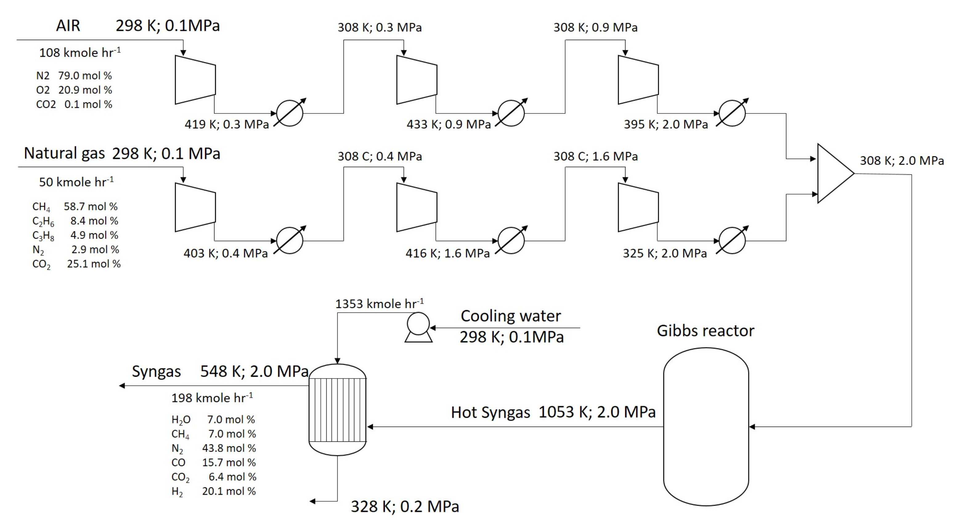
2.1. Process Simulation

The following description applies to the landfill gas and the biogas scenarios as well. A Python 3.9.4 code selects the composition of the sweet feedstock stream by a Monte Carlo analysis (Table 1) while its mole flow is set to 50 kmol h−1 (approximately 20 m3 min−1 see Supporting Materials). The MRU scale is larger compared to the Canadian production, but falls in the 30th percentile of the permitted flaring of Texas oil producers [6,38]. The Soave–Redlich–Kwong (RKS) equation of state calculates the fugacities of the components [39]. Aspen v.11 calculated the mass and energy balances for the two compressors (methane-rich gas and air) and the CPOX reactor, which we simulated as a Gibbs reactor. The compression ratio of the reciprocal compressors should be lower than 5 [40], with a maximum outlet temperature below 433 K therefore, we simulated three sequential one-stage intercooled compressors for each stream to meet these specifications. The outlet pressure of both compressors is 2 MPa. A design specification (Design/Spec) fixes the molar ratio of carbon and oxygen in the stream entering in the CPOX reactor equal to 2 by adjusting the flowrate of air (simulated as a mixture of 21% of O2 and 79% of N2). A thermodynamic analysis individuated the best ratio to be 1.7 [24,25] to minimize the coke formation. However, here we assumed the stoichiometric ratio because the objective was not to optimize the catalyst formulation to minimize coke formation.
The CPOX reactor operates at 2 MPa and we assumed a negligible pressure drop across the catalytic bed. Some of the authors optimized this configuration in a previous work [25]. We simulated an adiabatic Gibbs reactor. CPOX converts the gas into CO and H2 (plus H2O and CO2). The outlet temperature of the CPOX reactor ranges from 933 K to 1033 K. A heat exchanger (shell and tube), with an exchange area of 1.834 m2, reduces the temperature of this stream to 548 K. We fixed its value to S + 2ΔS, where S and ΔS are the average heat exchange area and its standard deviation obtained by 50 simulations changing the gas composition, respectively. Water at 298 K is the utility stream for the heat exchanger.
We coded the kinetics of the FT reaction in Python 3.9.4. We employed a model that considers an iron catalyst and calculates the paraffin, olefin and alcohol distributions based on 7 micro-kinetics rate steps [41]. The model also considers the water–gas shift reaction (see Supporting Information). We assumed a residence time of 1.6 min and calculated CO conversion, product distribution ( α ) and the ratio between hydrocarbons and olefins and alcohols.
The Python 3.9.4 program iteratively solves the Aspen flowsheet and the FT reactor, changing the initial feed gas composition 3000 times (Figure 2). It then stores the results of each cycle in an Excel file, that calculates the distribution of the output variables. These values, with their uncertainties, passed to the techno-economic analysis.

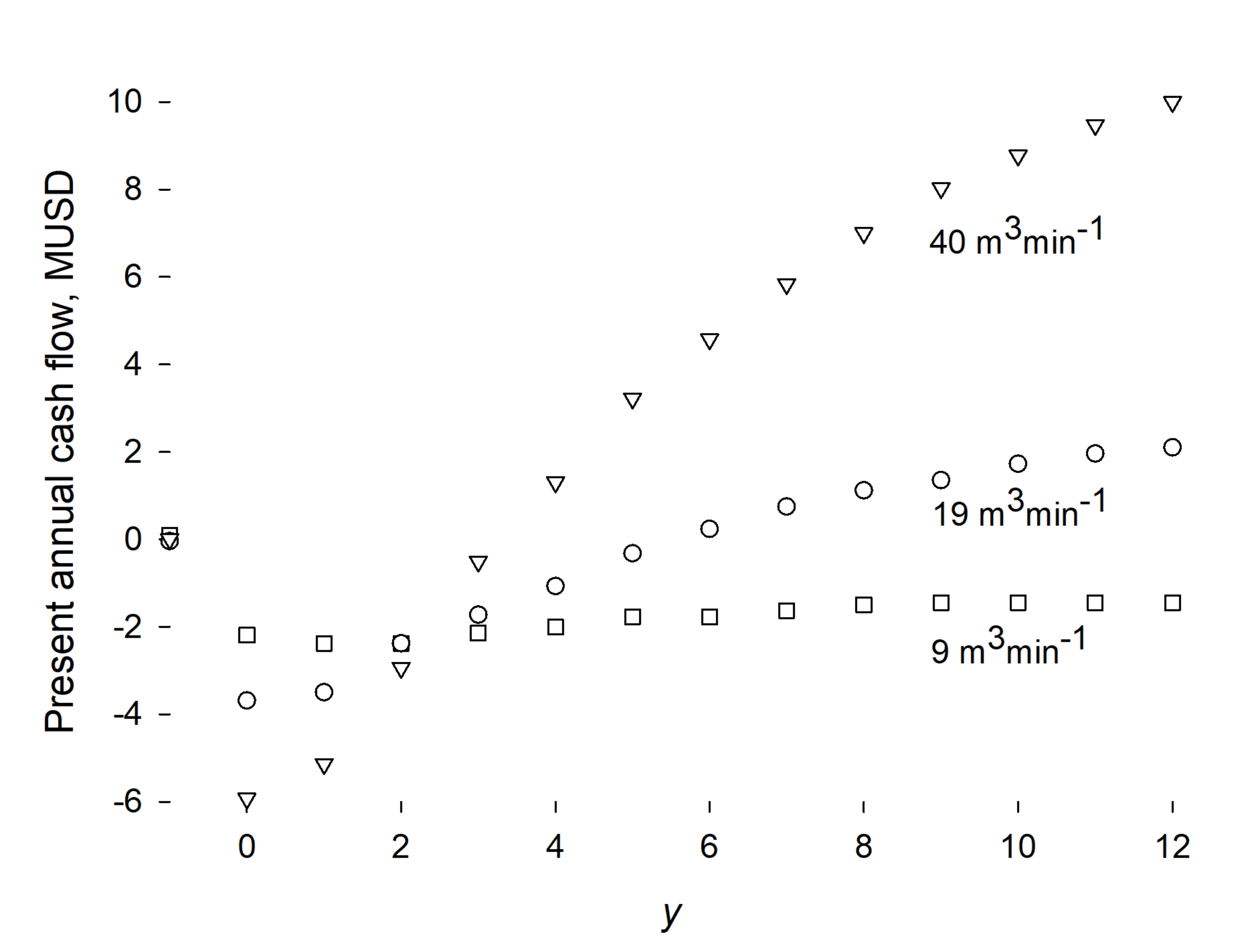
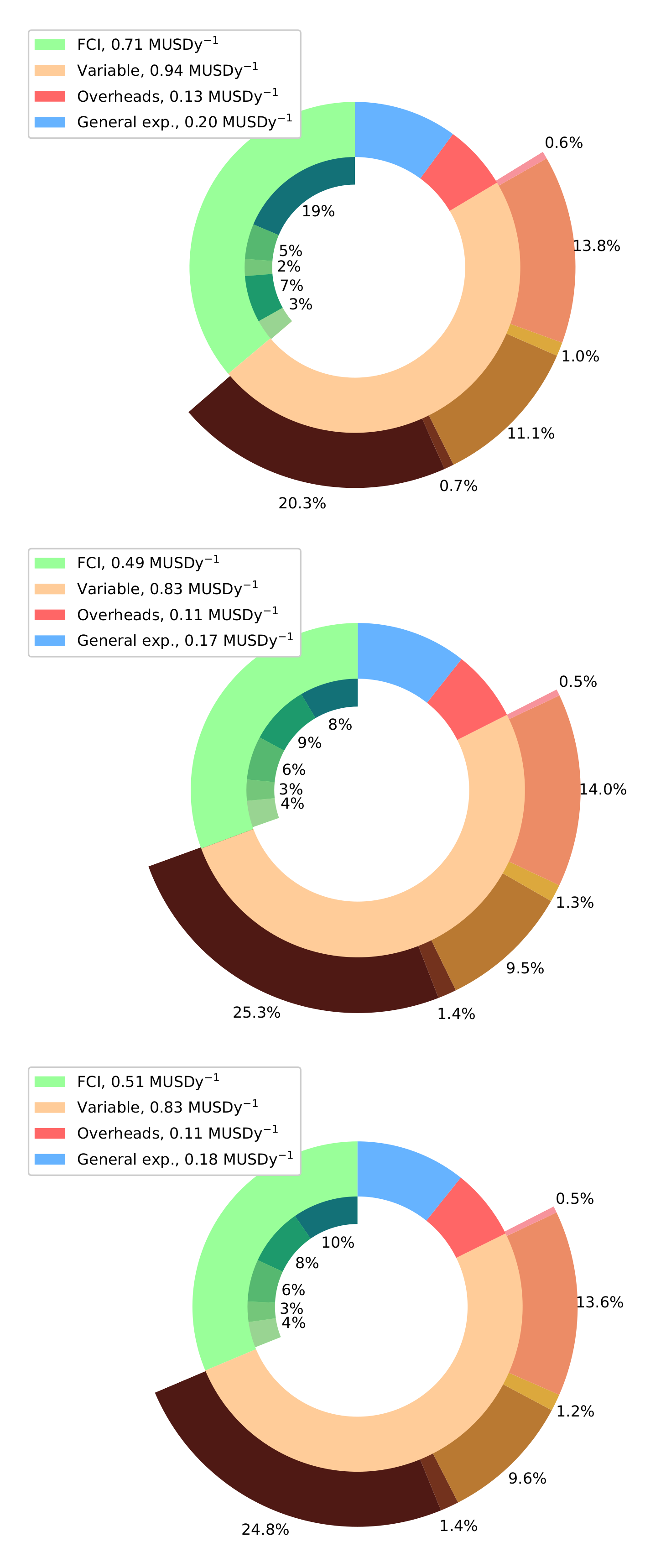
2.2. Techno-Economic Analysis

First, we calculated the capital cost for each equipment, and then the total capital investment (TCI) as the sum of direct capital cost, indirect capital, cost and working capital. Then, we estimated the profitability of each scenario via the Net Present Value (NPV) [46]. We selected reciprocal piston stainless steel compressors for both air and methane-rich feedstock. The pump for cooling water is a reciprocal stainless steel pump. For CPOX and FT reactors, we employed stainless steel vessels with an inner diameter of 0.5 m and 1 m, respectively. The height of the CPOX and FT reactor is 1 m and 6 m, respectively.
Empirical correlations estimated the cost of unit operations ( C BM , i ), the purchase price ( C P , i ) and the bare module factor ( F BM , i ) [47] (CEPCI2004 = 400). We actualized the cost of the equipment using the 2020 CEPCI index (Equation (1), 618.7 for heat exchangers and reactors, and 1080.2 for compressors and pumps) [48,49]
C BM , i = C P , i · F BM , i · CEPCI 2020 400
A second Python 3.9.4 algorithm generates the averages and standard deviations of compressors’ duties, pump duty, cooling water flow rate, and FT product flowrate and composition. From these, it calculates the cost of the equipment [47] and the total capital investment ( T C I ). T C I includes the direct capital costs ( C Direct ) as well as the indirect capital costs ( C Indirect ), and working capital costs ( W C ) (Equation (2)):
T C I = F C I + W C W C = ( C Pur + C Del ) · 0.05 C Pur = i = 1 N C BM , i C Del = C Pur · 0.1 F C I = C Direct + C Indirect C Direct = ( C Pur + C Del ) · ( 1 + f Inst + f Instr + f Pipe + f Elec + f Buil + f Fac + f Impr ) C Indirect = ( C Pur + C Del ) · ( 1 + f Eng + f Constr + f Leg + f Fee + f Cont )
The direct capital costs include purchased equipment installation ( f Inst ), instrumentation and controls ( f Instr ), piping ( f Pipe ), electrical systems ( f Elec ), building ( f Buil ), yard improvement ( f Impr ), and service facilities ( f Fac ). The indirect capital costs include engineering and supervision ( f Eng ), construction expenses ( f Constr ), legal expenses ( f Leg ), the contractor’s fee ( f Fee ), and contingency ( f Cont ). We assigned a factor to calculate these costs (Table 2, Equation (2)).
The plant benefits from an accelerated depreciation over 5 y: 20% the first year, then in an sum-of-the-years’ digits method for the remaining 4 y. We considered electricity, waste disposal, and cooling water as utilities.
Variable costs ( C VAR ) include labor costs ( C Lab ), supervision ( C Sup ), maintenance ( C Main ), supplies ( C Supp ), laboratory and research ( C Res ), royalties ( C Roy ), catalyst ( C Cat ), and utilities ( C Ut ), as shown in Equation (3). For labor costs, we assumed 1 operator per shift over four shifts per day. Since the MRU integrates an already existing plant, one additional operator is enough to operate the unit. The operator cost is 34 USD h−1. The annual operating labor cost is 0.295 MUSD y−1. Concerning utilities, the electricity cost is 0.012 USD kW−1 [50]. The waste disposal cost includes the hazardous (145 USD t−1) and non-hazardous materials (36 USD t−1) [51,52]. We assumed that both the hazardous component and the non-hazardous component account for 1% of the whole product [46]. The cooling water cost is 0.08 USD m3 and we only accounted for the make up water. In particular, we calculated the make up water flowrate as 0.2%/K [46,53] of the cooling water mass flowrate considering the temperature difference between the inlet and outlet of the heat exchanger. We also accounted for the carbon dioxide emission cost (50 USD t−1):
C VAR = C Lab + C Sup + C Main + C Supp + C Res + C Roy + C Cat + C Ut C Sup = C Lab · 0.05 C Main = F C I · 0.06 C Supp = C Main · 0.05 C Res = C Lab · 0.05 C Roy = 0 C Cat = Yearly Catalyst · Product price · 0.005
We set royalties to zero because the unit is internal proprietary technology [54].
Regarding raw material and product prices, we devised nine different cases that represent the optimal (Case 3), average, and worst case (Case 1) scenarios (Table 3).
To the variable costs, we added fixed charges as ( C Charges ): taxes ( C Tax ), financing ( C Fin ), insurance ( C Insu ), and renting material ( C Rent ) —and plant overheads( C Overhead ), as illustrated in Equation (4):
C Charges = C Tax + C Fin + C Insu + C Rent + C Overhead C Tax = F C I · 0.02 C Fin = 0 C Insu = F C I · 0.01 C Rent = 0 C Overhead = ( C Lab + C Sup + C Main ) * 0.2
We assume zero financing and renting costs because we did not consider lending money for the construction of the MRU and there is no need to rent further equipment. Eventually, we considered general expenses ( C General ), constituted by administrative expenses ( C Admin ), distribution and selling ( C Distr ), and development ( C Devel )—as illustrated Equation (5):
C General = C Admin + C Distr + C Devel C Admin = ( C Lab + C Sup + C Main ) · 0.1 C Distr = ( C Admin + C Overhead + C Charges + C VAR C Roy C Cat ) · 0.05 C Devel = ( C Admin + C Overhead + C Charges + C VAR C Roy C Cat ) · 0.05
For the calculation of the net return and the payback time, we assumed an inflation rate of 2% and an income tax of 28%, which is conservative in Canada, whose taxation is from 11.5% to 16% depending on the province [57], but it is in line with the rest of the Western nations. Eventually, we considered that the MRU operates at 0% capacity the first year (−1) (we considered construction and installation), then at 50%, 90%, 100% each progressive successive year. We applied a yearly present worth factor (PWF) of 13% for the calculation of the NPV (Table 4).

3. Results and Discussion

The MRU produces a syngas whose H2/CO ratio is understoichiometric, due to the presence of CO2 and higher hydrocarbons in the feedstock (from 0.7–1.7, as shown in Figure 3).
The high concentration of CO2 in landfill gas limitS hydrogen production for the co-presence of the dry reforming reaction that is endothermic and produces an equimolar mixture of CO and H2 [58]. In this scenario, the CPOX reactor of the MRU operates more as an autothermal dry reformer with an excess of oxygen. Indeed, the equilibrium temperature reached in the Gibbs reactor depends on the content of CO2, ranging from 973K to 1123 K (Figure S1b in Supporting Information). Similarly, the most likely value of the CO conversion in the Fischer–Tropsch reactor follows the same trend, ranging from 50% to 65%, which are values that agree with single-pass FT reactors [59].
For NG, we calculated a hydrocarbon production of 1,956,100 kg y−1. However, the MRU is only economical when we discount the carbon tax for the avoided flaring, with a payback time ranging from (0.71 ± 0.11) y to (0.66 ± 0.09) y depending on the product price assumed. It is difficult to compare our results to those in the literature because, as explained in the introduction, there are not so many techno-economic models and most of them focus on large-scale units.
A sensitivity analysis (Table 5) on the production of hydrocarbons revealed that an iron catalyst is unsuitable to achieve an economical payback time because of its higher selectivity towards C1–C3 products. The production to have a payback time lower than 10 y is 7.3 kt y−1. A cobalt-based catalyst is therefore preferred for GtL units because of its higher intrinsic activity [60,61]. We continued our analysis accordingly, assuming a production of 1 × 10 3 kt y−1.
Under the most probable operating conditions (2–2, shown in Table 3), the natural gas scenario is economically the most interesting. When the natural gas feedstock is available at a price of zero, and when the liquid product sells similarly to crude oil, the cumulative NPV goes towards zero after 3.5 y, even with an accelerated depreciation of 5 years. This demonstrates that a portable, modular MRU plant, is economically self-sufficient without any direct (investment) or indirect (on the avoided emission) subsidy. After all the expenses, the MRU produces enough liquid to pay for carbon taxes for the CO2 emissions related to the combustion of the remaining flue gases. Oil and gas companies as well as local governments must at least aim to achieve this chemistry (CO conversion, product distribution), and these economics to operate their wells. Even more interesting is the case where the natural gas feedstock comes with a negative price, equivalent to the avoided carbon emissions. With the carbon tax increasing in the near future, this case will be even more beneficial.
The nature of the feedstock does not heavily affect the economics. The MRU performs better for feedstocks richer in methane, but at the same time, it operates quite well over wide range of natural gas compositions (Figure 3).
Emissions from flared stranded gas pose the main threat (in terms of volumes) to the environment. We optimized our operating conditions (H2/CO ratio) for this feedstock source. By injecting water, or by simply changing the air intake, the biogas and the landfill cases could be more viable. Moreover, steam condensation requires additional CAPEXs and OPEXs due to heat tracing. However, our ultimate objective was to benchmark the three cases in the easiest manner, to demonstrate that the process is attractive even when the best possible outcome is not achieved.
We studied the influence of the scale of the MRU, changing the natural gas flowrate to 25 kmol h−1 (approximately 9 m 3 min−1, lower scale) and 100 kmol h−1 (approximately 40 m 3 min−1, higher scale). In the actual economic scenario, the reduced production due to a lower gas flow is insufficient to have a positive net present value, even if CAPEXs are 60% compared to the base scale analyzed (natural gas flared flowrate of 19 m 3 min−1, as shown in Figure 4).
MRU benefits to some extent from the economies of the scale. Even if the CAPEXs and OPEXs increase accordingly, higher production reduces the payback time if we assume a natural gas flowrate of 40 m 3 min−1 (Table 6). This flowrate represents approximately 25 % of the Texas permitted flares in 2010 [38].
Similarly, MRU benefits from numbering up [62,63]. The unit itself needs minimum maintenance, control and supervision, and runs lean in terms of personnel and direct and indirect capital cost expenses (Equation (2)). This is because of its small scale and its modularity [18]. A bigger plant is not portable and needs at least one extra operator, plus higher direct and indirect capital costs (5.9 MUSD for the case where we considered 40 m 3 min−1 of natural gas flared instead of a total of 37 MUSD for the base case, Equation (2)). Furthermore, the attractiveness goes with a quick payback time and a relatively cheap plant. This way, oil companies can approach the increasing carbon tax and public concern in a timely manner, whilst having a delocalized unit that they build over one year, depreciate in five, and dismantle and move between wells at low cost. The same applies in the case of landfills and biogas in remote places, where local authorities need a simple, affordable, and modular plant to address the environmental threats of uncontrolled emissions.
We foresee the MRU as a lean plant, where the investment itself plays the biggest impact on annual expenses (Figure 5). Compressors represent the main source of fixed costs for the MRU, with 70 ± 8%, 71 ± 8%, and 57 ± 3% for natural gas, biogas, and landfill gas, respectively. For natural gas, the bare module model overestimates the cost of the air compressor (USD 562,000 ± USD 42,000) because the empirical regressions only account for the unit duty (Figure 5). In the other two scenarios, both the compressors were estimated to cost between USD 200,000 to USD 210,000 (including installation, control, etc.), which is more reasonable (Figure 5). The model estimates the reactors’ cost at USD 170,000, which represent between 11% and 14% of the purchase costs. The total fixed investment resulted in 2.7 MUSD, 3.3 MUSD, and 4.7 MUSD for landfill gas, biogas, and natural gas (Figure 5), respectively (uncertainty below 1%). Utilities account for between USD 200,000 y 1 and USD 270,000 y 1 with waste disposal as the main source of cost (waste disposal is proportional to annual production).
According to the rule of thumb which says that FT-based GtL units cost (FCIs) approximately 100,000 USD bbl 1 d of production [16], we calculated that our unit respects this estimation for the biogas and landfill scenario (USD 95,000 bbl 1 d to USD 105,000 bbl 1 d), while for the natural gas, the overestimation of the FCI costs for compressor is a bias.
We designed and simulated a CPOX reactor with a stoichiometric hydrocarbon/oxygen ratio. With this configuration, the biogas and the landfill gas in the current economic scenario (case 2–2 of Table 3) resulted with a negative actual cash flow (Figure 6). The presence of CO2 and higher hydrocarbon reduces the total FT-fuel production. It is out of the scope of this paper to optimize the condition for both these methane-rich feedstocks, which, however, resulted in a slightly negative annualized actual cash flow: −3.8 MUSD and −4.4 MUSD in year y = 12 for biogas and landfill gas, respectively, with an initial investment of −2.5 MUSD and −2.6 MUSD. We speculate that the optimized operating conditions and oxidant feed (steam or using green hydrogen to increase the CO/H2 ratio in the FT reactor) also make the MRU economical for biogas and landfill gas, feedstocks that are suitable for GtL technologies [64,65,66].
A combined techno-economic assessment and LCA may also find that optimal operating conditions reduce emissions [67].

4. Conclusions

Flaring natural gas is the only solution for battery units in remote locations. However, environmental concerns and new GtL processes create new avenues to solve this issue. The MRU integrates the existing flaring sites on the well and converts 40% to 75% of the stranded gas into liquid hydrocarbons, which are an extra source of revenue for producers. The MRU has a payback time of less than 10 years regardless of the assumed fuel price. On the other hand, if we consider the stranded gas to cost the same as natural gas, or the MRU to treat less than 10 m 3 min−1, the technology we propose is not viable. The oil industry is mercurial, and the stability of production, safety, technology maturity, and oil price are the major sources of uncertainty. Moreover, the chemical industry should strive towards plant automatization, as a part of the accelerated development of the 4.0 technologies [68]. In the North American context, regional or provincial bodies can either decide to grant incentives up-front on the CAPEXs, or alternatively, focus on the final product. We did not account for governmental economic incentives that reduce CAPEXs from 30% to 50% (and their relative depreciation) in our calculation. We also neglected a scenario where local bodies decide to subsidize the FT liquid itself. This last scenario is particularly appreciated by the local authorities, because it can decide to bet only on winning technologies, is mature enough to ensure steady operation and production in the long term. A third kind of incentive is the carbon tax, planned to increase to 135 USD by 2030, becoming the biggest contributor to the NPV of the plant. Concerning the Fischer–Tropsch synthesis, Co or Rh are more indicative compared to iron-based catalysts due to their higher α and CO per-pass conversion. MRU is also economical with feedstock such as biogas or landfill gas, which will become the main source of carbon when the energetic transition towards renewables will be achieved.

Supplementary Materials

The following are available online at https://www.mdpi.com/article/10.3390/pr9091568/s1, Figure S1: Comparison between the calculated kinetic constants from our Python model and the experimental data at 573 K. Paraffin formation (a), olefins absorption (b), and alcohols desorption (d) show good agreement with the experimental data. The olefins desorption step (c) resulted as underestimated because the value of the parameter α P , HC 6 re was not reported in the manuscript. We assumed α P , HC 6 re = 1 α P , HC 6 . Moreover, the value of E0HC6re is not present in Table 6. We assumed E 0 , HC 6 re = E 0 , HC 6 (lines 30–31 of kinetics.py), Figure S2: Distributions of the feedstock compressor duty (a), CPOX temperature (b), H2/CO ratio in syngas (c), CO conversion in the FT reactor (d), and asf chain growth probability factor (e) for the three scenarios, Code—Python.rar: Source code of the Python algorithm.

Author Contributions

Conceptualization, F.G. and J.D.T.; methodology, F.G., J.-J.L. and J.D.T.; software, F.G. and J.-J.L.; validation, F.G., J.D.T., G.P. and G.S.P.; formal analysis, F.G.; resources, G.S.P.; data curation, F.G. and G.S.P.; writing—original draft preparation, F.G., J.-J.L. and J.D.T.; writing—review and editing, F.G., G.P. and G.S.P.; visualization, F.G. and G.S.P.; supervision, G.S.P. and F.G.; funding acquisition, G.S.P. All authors have read and agreed to the published version of the manuscript.

Funding

This research was undertaken, in part, thanks to funding from the Canada Research Chair program and Canada Foundation for Innovation. J.-J.L. received the “2021 Winter Research Internship Program” scholarship funded by Polytechnique Montreal— project number WRIP21, Project 17: GtL micro-refinery unit: conversion of methane into liquid hydrocarbons. Supervised by Pr. Gregory Patience.

Institutional Review Board Statement

Not applicable.

Informed Consent Statement

Not applicable.

Data Availability Statement

The data presented in this study are available in the article and the Supplementary Materials.

Conflicts of Interest

The authors declare no conflict of interest.

Abbreviations

The following abbreviations are used in this manuscript:
AERAlberta Energy Regulator
ASUAir separation Unit
CAPEXsCapital expenses
CEPCIChemical engineering plant cost index
CPOXCatalytic partial oxidation
EPAEnvironmental Protection Agency
FCIsFixed capital investments
FTFischer–Tropsch
GtLGas to liquid
LNGLiquefied natural gas
MRUMicro refinery unit
NGNatural gas
NPVNet present value
OPEXsOperating expenses
PWFPresent worth factor
TCITotal capital investment
WGSWater–gas shift

References

  1. US Energy Information Administration. Upstream Petroleum Industry Flaring and Venting Report Industry Performance for Year Ending 31 December 2019. 2020. Available online: https://static.aer.ca/prd/documents/sts/ST60B-2020.pdf (accessed on 11 April 2021).
  2. Edenhofer, O. Climate Change 2014: Mitigation of Climate Change; Cambridge University Press: Cambridge, MA, USA, 2015; Volume 3. [Google Scholar]
  3. Derwent, R.G. Global Warming Potential (GWP) for Methane: Monte Carlo Analysis of the Uncertainties in Global Tropospheric Model Predictions. Atmosphere 2020, 11, 486. [Google Scholar] [CrossRef]
  4. European Commission. Reducing Greenhouse Gas Emissions: Commission Adopts EU Methane Strategy as Part of European Green Deal. 2020. Available online: https://ec.europa.eu/commission/presscorner/detail/en/ip_20_1833 (accessed on 21 July 2021).
  5. European Commission. Reducing Methane Emissions: Opportunities and Barriers in Waste and Agriculture through Biogas Production. 2020. Available online: https://ec.europa.eu/info/events/reducing-methane-emissions-opportunities-and-barriers-waste-and-agriculture-through-biogas-production-2020-jul-17_en (accessed on 21 July 2021).
  6. US Energy and Information Administration. PETROLEUM & OTHER LIQUIDS. 2021. Available online: https://www.eia.gov/dnav/pet/hist/LeafHandler.ashx?n=pet&s=mcrfpus2&f=m (accessed on 11 April 2021).
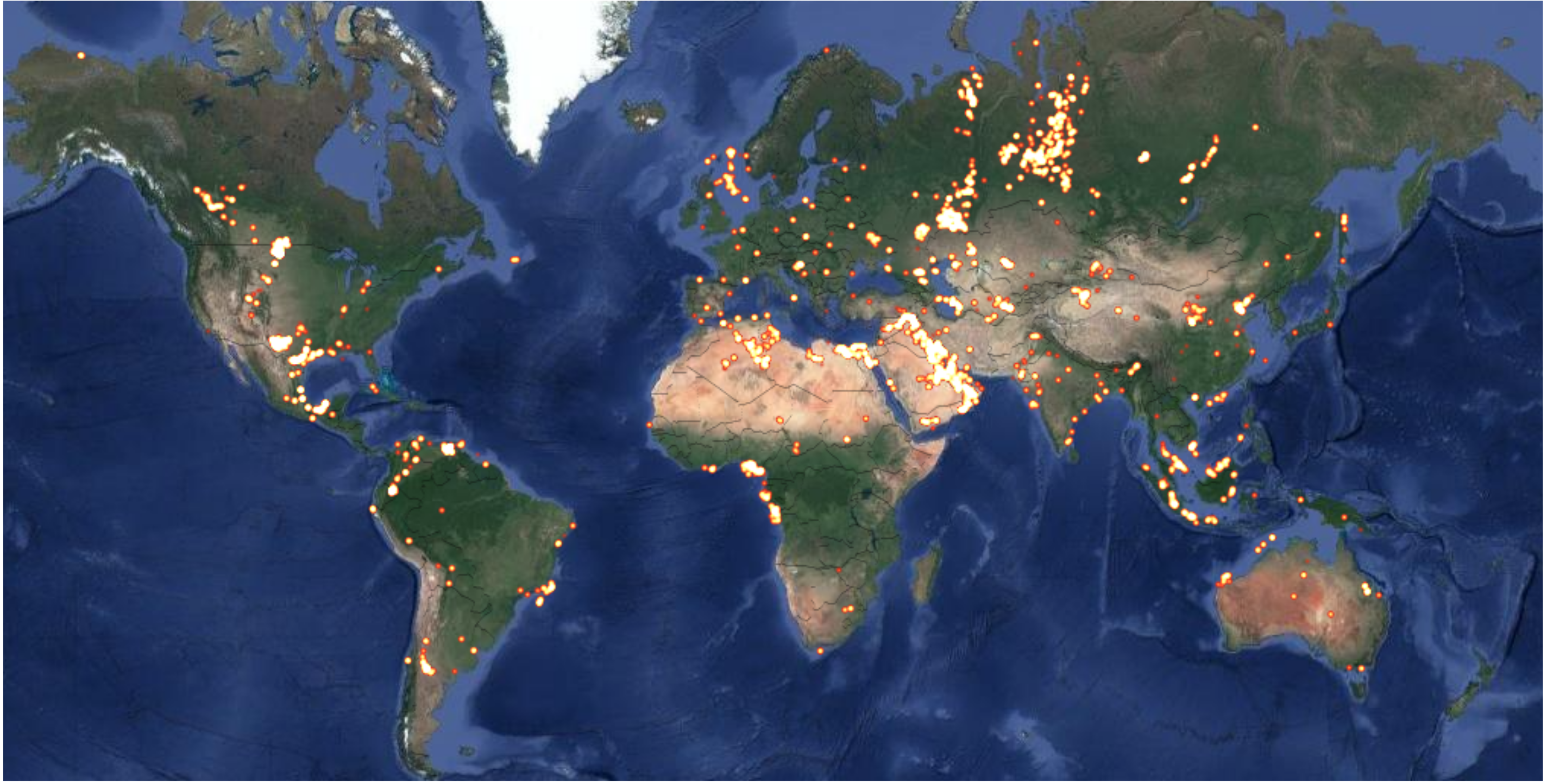
  7. Skytruth. Satellite-Detected Natural Gas Flaring. 2020. Available online: https://skytruth.org/flaring/ (accessed on 7 June 2021).
  8. Government of Canada. How Carbon Pricing Works. 2021. Available online: https://www.canada.ca/en/environment-climate-change/services/climate-change/pricing-pollution-how-it-will-work/putting-price-on-carbon-pollution.html (accessed on 21 July 2021).
  9. CompactGTL. CompactGTL’s Project in Kazakhstan. 2018. Available online: http://www.compactgtl.com/about/projects/ (accessed on 17 February 2021).
  10. Greyrock. Technology Greyrock Chemical and Fuel Production. 2008. Available online: http://www.greyrock.com/technology/ (accessed on 17 February 2021).
  11. Hargreaves, N. Roll out of Smaller Scale GTL Technology at ENVIA Energy’s Plant in Oklahoma City, USA. 2017. Available online: https://www.velocys.com/press/ppt/Gastech2017_Velocys_FINAL_4.3_web.pdf (accessed on 2 March 2021).
  12. Infra. 2020. Available online: https://en.infratechnology.com/technology/RR# (accessed on 3 March 2021).
  13. Pirola, C.; Scavini, M.; Galli, F.; Vitali, S.; Comazzi, A.; Manenti, F.; Ghigna, P. Fischer–Tropsch Synthesis: EXAFS Study of Ru and Pt bimetallic Co Based Catalysts. Fuel 2014, 132, 62–70. [Google Scholar] [CrossRef]
  14. Di Michele, A.; Sassi, P.; Comazzi, A.; Galli, F.; Pirola, C.; Bianchi, C.L. Co- and Co(Ru)-Based Catalysts for Fischer-Tropsch Synthesis Prepared by High Power Ultrasound. Mater. Focus 2015, 4, 295–301. [Google Scholar] [CrossRef]
  15. Louyot, P.; Neagoe, C.; Galli, F.; Pirola, C.; Patience, G.S.; Boffito, D.C. Ultrasound-assisted impregnation for high temperature Fischer-Tropsch catalysts. Ultrason. Sonochemistry 2018, 48, 523–531. [Google Scholar] [CrossRef]
  16. Kanshio, S.; Agogo, H.O.; Chior, T.J. Techno-Economic Assessment of Mini-GTL Technologies for Flare Gas Monetization in Nigeria. In Proceedings of the SPE Nigeria Annual International Conference and Exhibition, Lagos, Nigeria, 1 July–2 August 2017. [Google Scholar] [CrossRef]
  17. Remer, D.S.; Chai, L.H. Design cost factors for scaling-up engineering equipment. Chem. Eng. Prog. 1990, 86, 77–82. [Google Scholar]
  18. Patience, G.S.; Boffito, D.C. Distributed production: Scale-up vs. experience. J. Adv. Manuf. Process. 2020, 2, e10039. [Google Scholar] [CrossRef]
  19. Mohajerani, S.; Kumar, A.; Oni, A.O. A techno-economic assessment of gas-to-liquid and coal-to-liquid plants through the development of scale factors. Energy 2018, 150, 681–693. [Google Scholar] [CrossRef]
  20. Collodi, G.; Azzaro, G.; Ferrari, N.; Santos, S. Demonstrating Large Scale Industrial CCS through CCU—A Case Study for Methanol Production. Energy Procedia 2017, 114, 122–138. [Google Scholar] [CrossRef]
  21. Banaszkiewicz, T.; Chorowski, M.; Gizicki, W. Comparative analysis of cryogenic and PTSA technologies for systems of oxygen production. AIP Conf. Proc. 2014, 1573, 1373–1378. [Google Scholar] [CrossRef]
  22. Dong, L.; Wei, S.; Tan, S.; Zhang, H. DGTL or LNG: Which is the best way to monetize ‘stranded’ natural gas? Pet. Sci. 2008, 5, 388–394. [Google Scholar] [CrossRef] [Green Version]
  23. Trevisanut, C.; Jazayeri, S.M.; Bonkane, S.; Neagoe, C.; Mohamadalizadeh, A.; Boffito, D.C.; Bianchi, C.; Pirola, C.; Visconti, C.G.; Lietti, L.; et al. Micro-syngas technology options for GtL. Can. J. Chem. Eng. 2016, 94, 613–622. [Google Scholar]
  24. Pauletto, G.; Mendil, M.; Libretto, N.; Mocellin, P.; Miller, J.T.; Patience, G.S. Short contact time CH4 partial oxidation over Ni based catalyst at 1.5MPa. Chem. Eng. J. 2021, 414, 128831. [Google Scholar] [CrossRef]
  25. Pauletto, G.; Galli, F.; Gaillardet, A.; Mocellin, P.; Patience, G.S. Techno economic analysis of a micro Gas-to-Liquid unit for associated natural gas conversion. Renew. Sustain. Energy Rev. 2021. [Google Scholar] [CrossRef]
  26. Zichittella, G.; Pérez-Ramírez, J. Status and prospects of the decentralised valorisation of natural gas into energy and energy carriers. Chem. Soc. Rev. 2021, 50, 2984–3012. [Google Scholar]
  27. Delborne, J.A.; Hasala, D.; Wigner, A.; Kinchy, A. Dueling metaphors, fueling futures: “Bridge fuel” visions of coal and natural gas in the United States. Energy Res. Soc. Sci. 2020, 61, 101350. [Google Scholar] [CrossRef]
  28. Yuan, X.C.; Lyu, Y.J.; Wang, B.; Liu, Q.H.; Wu, Q. China’s energy transition strategy at the city level: The role of renewable energy. J. Clean. Prod. 2018, 205, 980–986. [Google Scholar] [CrossRef]
  29. Baena-Moreno, F.M.; Pastor-Pérez, L.; Wang, Q.; Reina, T. Bio-methane and bio-methanol co-production from biogas: A profitability analysis to explore new sustainable chemical processes. J. Clean. Prod. 2020, 265, 121909. [Google Scholar] [CrossRef]
  30. Heo, J.; Lee, B.; Lim, H. Techno-economic analysis for CO2 reforming of a medium-grade landfill gas in a membrane reactor for H2 production. J. Clean. Prod. 2018, 172, 2585–2593. [Google Scholar] [CrossRef]
  31. Gao, R.; Zhang, C.; Lee, Y.J.; Kwak, G.; Jun, K.W.; Kim, S.K.; Park, H.G.; Guan, G. Sustainable production of methanol using landfill gas via carbon dioxide reforming and hydrogenation: Process development and techno-economic analysis. J. Clean. Prod. 2020, 272, 122552. [Google Scholar] [CrossRef]
  32. Statista. Leading Biogas Producing Countries in 2014. 2021. Available online: https://www.statista.com/statistics/481840/biogas-production-worldwide-by-key-country/ (accessed on 16 August 2021).
  33. International Energy Agency. The Outlook for Biogas and Biomethane to 2040. 2021. Available online: https://www.iea.org/reports/outlook-for-biogas-and-biomethane-prospects-for-organic-growth/the-outlook-for-biogas-and-biomethane-to-2040 (accessed on 16 August 2021).
  34. The World Bank. What a Waste 2.0. A Global Snapshot of Solid Waste Management to 2050. 2021. Available online: hdl.handle.net/10986/30317 (accessed on 16 August 2021).
  35. Mukherjee, R.; Reddy Asani, R.; Boppana, N.; El-Halwagi, M.M. Performance evaluation of shale gas processing and NGL recovery plant under uncertainty of the feed composition. J. Nat. Gas Sci. Eng. 2020, 83, 103517. [Google Scholar] [CrossRef]
  36. Basini, L.E.; Busto, C.; Villani, M. Process for the Production of Methanol from Gaseous Hydrocarbons. WO 2020/058859 A1, 9 July 2020. [Google Scholar]
  37. De Tommaso, J.; Rossi, F.; Moradi, N.; Pirola, C.; Patience, G.S.; Galli, F. Experimental methods in chemical engineering: Process simulation. Can. J. Chem. Eng. 2020, 98, 2301–2320. [Google Scholar] [CrossRef]
  38. US Department of Energy, Office of Oil and Natural Gas. Natural Gas Flaring and Venting: State and Federal Regulatory Overview, Trends, and Impacts. 2019. Available online: https://www.energy.gov/sites/prod/files/2019/08/f65/Natural%20Gas%20Flaring%20and%20Venting%20Report.pdf (accessed on 28 June 2021).
  39. Soave, G. Equilibrium constants from a modified Redlich-Kwong equation of state. Chem. Eng. Sci. 1972, 27, 1197–1203. [Google Scholar] [CrossRef]
  40. Mokhatab, S.; Poe, W.A. Handbook of Natural Gas Transmission and Processing; Gulf Professional Publishing: Waltham, MA, USA, 2012. [Google Scholar]
  41. Zhou, L.; Froment, G.F.; Yang, Y.; Li, Y. Advanced fundamental modeling of the kinetics of Fischer–Tropsch synthesis. AIChE J. 2016, 62, 1668–1682. [Google Scholar] [CrossRef]
  42. Johnson, M.; Kostiuk, L.; Spangelo, J. A Characterization of Solution Gas Flaring in Alberta. J. Air Waste Manag. Assoc. 2001, 51, 1167–1177. [Google Scholar] [CrossRef] [Green Version]
  43. Berger, S.; Dun, S.; Gavrelis, N.; Helmick, J.; Mann, J.; Nickle, R.; Perlman, G.; Warner, S.; Wilhelmi, J.; Williams, R.; et al. Landfill Gas Primer: An Overview for Environmental Health Professionals; ATSDR: Atlanta, GA, USA, 2001. [Google Scholar]
  44. Li, Y.; Alaimo, C.P.; Kim, M.; Kado, N.Y.; Peppers, J.; Xue, J.; Wan, C.; Green, P.G.; Zhang, R.; Jenkins, B.M.; et al. Composition and Toxicity of Biogas Produced from Different Feedstocks in California. Environ. Sci. Technol. 2019, 53, 11569–11579. [Google Scholar] [CrossRef]
  45. Ammenberg, J.; Bohn, I.; Feiz, R. Systematic Assessment of Feedstock for an Expanded Biogas Production: A Multi-Criteria Approach. 2017. Available online: http://www.diva-portal.org/smash/record.jsf?pid=diva2%3A1156008&dswid=4879 (accessed on 5 May 2021).
  46. Green, D.W.; Southard, M.Z. Perry’s Chemical Engineers’ Handbook; McGraw-Hill Education: San Francisco, CA, USA, 2019. [Google Scholar]
  47. Ulrich, G.D.; Vasudevan, P.T. Chemical Engineering Process Design and Economics: A Practical Guide; Process Publishing: New York, NY, USA, 2003. [Google Scholar]
  48. Vatavuk, W.M. Updating the CE Plant Index. 2002. Available online: https://www.chemengonline.com/Assets/File/CEPCI_2002.pdf.
  49. Jenkins, S. 2021 CEPCI UPDATES: FEBRUARY (PRELIM.) AND JANUARY (FINAL). 2021. Available online: https://www.chemengonline.com/2021-cepci-updates-february-prelim-and-january-final/ (accessed on 5 May 2021).
  50. Sönnichsen, N. Canada’s Average Industrial Electricity Prices by major City 2019 by Select City (in Canadian Cents per Kilowatt Hour). 2020. Available online: https://www.statista.com/statistics/579159/average-industrial-electricity-prices-canada-by-major-city/ (accessed on 5 May 2021).
  51. Town of Calgary. Landfill Rates. 2021. Available online: https://www.calgary.ca/uep/wrs/landfill-information/landfill-rates.html (accessed on 5 May 2021).
  52. Town of Edmonton. Waste Management Fees & Rates. 2021. Available online: https://www.edmonton.ca/programs_services/garbage_waste/rates-fees.aspx (accessed on 5 May 2021).
  53. Vengateson, U. Cooling Towers: Estimate Evaporation Loss and Makeup Water Requirements. 2020. Available online: https://www.chemengonline.com/cooling-towers-estimate-evaporation-loss-and-makeup-water-requirements/?printmode=1 (accessed on 5 May 2021).
  54. Patience, G.; Boffito, D.C. Method and Apparatus for Producing Chemicals from a Methane-Containing Gas. U.S. Patent 9,243,190, 26 January 2016. [Google Scholar]
  55. American Petroleum Institute. Gasoline, Diesel and Crude Oil Prices. 2021. Available online: https://gaspricesexplained.com/#/?section=gasoline-diesel-and-crude-oil-prices (accessed on 5 May 2021).
  56. Index Mundi. Crude Oil, Average Spot Price of Brent, Dubai and West Texas Intermediate, Equally Weighed. 2021. Available online: https://www.indexmundi.com/commodities/?commodity=crude-oil (accessed on 5 May 2021).
  57. TaxTips.ca. 2020 Corporate Income Tax Rates. 2021. Available online: https://www.taxtips.ca/smallbusiness/corporatetax/corporate-tax-rates-2020.htm (accessed on 6 May 2021).
  58. Ponugoti, P.V.; Janardhanan, V.M. Mechanistic Kinetic Model for Biogas Dry Reforming. Ind. Eng. Chem. Res. 2020, 59, 14737–14746. [Google Scholar] [CrossRef]
  59. Raje, A.; Inga, J.R.; Davis, B.H. Fischer-Tropsch synthesis: Process considerations based on performance of iron-based catalysts. Fuel 1997, 76, 273–280. [Google Scholar] [CrossRef]
  60. Dancuart, L.; Steynberg, A. Fischer-Tropsch Based GTL Technology: A New Process. In Fischer-Tropsch Synthesis, Catalyst and Catalysis; Studies in Surface Science and Catalysis; Davis, B., Occelli, M., Eds.; Elsevier: Amsterdam, The Netheralnds, 2007; Volume 163, pp. 379–399. [Google Scholar] [CrossRef]
  61. Teimouri, Z.; Abatzoglou, N.; Dalai, A.K. Kinetics and Selectivity Study of Fischer–Tropsch Synthesis to C5+ Hydrocarbons: A Review. Catalysts 2021, 11, 330. [Google Scholar] [CrossRef]
  62. Bhosekar, A.; Ierapetritou, M. A framework for supply chain optimization for modular manufacturing with production feasibility analysis. Comput. Chem. Eng. 2021, 145, 107175. [Google Scholar] [CrossRef]
  63. Weber, R.S.; Askander, J.A.; Barclay, J.A. The scaling economics of small unit operations. J. Adv. Manuf. Process. 2021, 3, e10074. [Google Scholar]
  64. Okeke, I.J.; Mani, S. Techno-economic assessment of biogas to liquid fuels conversion technology via Fischer-Tropsch synthesis. Biofuels Bioprod. Biorefining 2017, 11, 472–487. [Google Scholar] [CrossRef]
  65. Hernandez, B.; Martin, M. Optimization for biogas to chemicals via tri-reforming. Analysis of Fischer-Tropsch fuels from biogas. Energy Convers. Manag. 2018, 174, 998–1013. [Google Scholar] [CrossRef]
  66. Zhao, X.; Naqi, A.; Walker, D.M.; Roberge, T.; Kastelic, M.; Joseph, B.; Kuhn, J.N. Conversion of landfill gas to liquid fuels through a TriFTS (tri-reforming and Fischer–Tropsch synthesis) process: A feasibility study. Sustain. Energy Fuels 2019, 3, 539–549. [Google Scholar]
  67. Galli, F.; Pirola, C.; Previtali, D.; Manenti, F.; Bianchi, C.L. Eco design LCA of an innovative lab scale plant for the production of oxygen-enriched air. Comparison between economic and environmental assessment. J. Clean. Prod. 2018, 171, 147–152. [Google Scholar] [CrossRef]
  68. Ramasamy, C.; Chun, T.H.; Kee, C.M.; Fong, G.T. Industrial Revolution 4.0 Contribution of chemical engineer. Turk. J. Comput. Math. Educ. (TURCOMAT) 2021, 12, 5037–5041. [Google Scholar]
Figure 1. Satellite-detected natural gas flared in June 2020 over a 30-day span—obtain from SkyTruth [7].
Processes 09 01568 g001
Figure 2. Schematic flowsheet of the simulation. The results reported represent one of the 3000 Monte Carlo cycles performed by the Python code. A complete list of all the simulated results for the three scenarios is available in the Supporting Materials.
Processes 09 01568 g002
Figure 3. Three thousand Monte Carlo iterations calculating the distribution of the hydrogen/carbon monoxide molar ratio after the CPOX unit for the three feedstocks considered.
Processes 09 01568 g003
Figure 4. The MRU is uneconomical for battery units that flare less than 10 m 3 min −1 of natural gas. Here, the FT fuel is sold at the same price as raw oil and the natural gas cost is 0 USD m−3 (scenario 2–2).
Processes 09 01568 g004
Figure 5. Depreciation of fixed capital investments (FCIs) per year (linear depreciation over 5 y), Variable costs, plant overheads and general expenses (administration distribution, selling, and R&D) for the MRU in the base case scenario with the three feedstocks (price = 0 USD y−1 and FT fuel price 0.3 USD kg−1). We outlined the contribution percentage of the main units to the FCIs (air compressor, natural gas compressor, water pump, CPOX reactor, FT reactor) and to variable costs (labor, catalyst,maintenance, supervision, utilities, and supplies). Top: natural gas; middle: biogas; bottom: landfill gas.
Processes 09 01568 g005
Figure 6. Present annual cash flow of the MRU for the three feedstocks studied. Lines represent the best possible scenario (cost of feedstock discounted by the carbon tax (−50 USD t−1 g CO2eq) and an FT fuel price of 0.2 USD kg−1); and the worst possible scenario (cost of feedstock of 0.23 USD kg −1 and an FT fuel price of 0.4 USD kg−1). Symbols represent the base-case scenario (cost of feedstock of 0 USD kg−1 and an FT fuel price of 0.3 USD kg−1).
Processes 09 01568 g006
Table 1. Composition distribution in the mole % for natural gas, landfill gas, and biogas. We assumed a triangular distribution for natural gas and a normal distribution for landfill gas. For each Monte Carlo cycle, Python 3.9.4 initializes the composition of the feedstock according to the probability distribution of each component and then normalizes the values to 100%.
Natural Gas [42]Landfill Gas [43]Biogas [44,45]
MinMost Likely ValueMax μ σ μ σ
CH419.29.099.552.52.548.05.8
C2H60.09.893.50.00.00.00.0
C3H80.05.841.00.00.00.00.0
N20.03.480.23.50.516.46.7
CO20.02.939.750.03.331.94.1
O20.00.00.00.50.23.82.1
CO0.00.00.00.10.030.00.0
Table 2. Capital cost factors.
ItemFraction of Delivered Equipment, ( C Pur + C Del )
Purchased Equipment Installation, f Inst 0.15
Instrumentation and Controls, f Instr 0.36
Piping, f Pipe 0.16
Electrical Systems, f Elec 0.10
Building, f Buil 0.00
Service Facilities, f Fac 0.30
Yard Improvement f Impr 0.00
Engineering and Supervision, f Eng 0.01
Construction Expenses, f Constr 0.34
Legal Expenses, f Leg 0.04
Contractor’s Fee, f Fee 0.17
Contingency, f Cont 0.32
Table 3. Our model evaluates the payback period and the net return after 10 y, considering feedstock and product prices variation.
Case
Value123
Feedstock Price0.23 USD kg−1 [55]0−50 tCO2eq In Feed,
USD
Product Price
(USD kg−1)
0.20.30.4 [56]
Table 4. Present worth factor applied (value of USD 1 at year y). Year 0 corresponds to the start of the operation.
Year−10123456789101112
PWF1.21.10.90.80.70.60.50.50.40.40.30.30.20.2
Table 5. Payback time ( P T , y ) correlates with the hydrocarbon production (P, kg y−1), ln ( P T ) = 28790000 ± 2036000 P 1.64 ± 0.21 , R 2 = 0.97 . With a production of 1.05 × 10 7 kg y−1, the MRU breaks—even 3 y after its installation.
CaseProduction, kg y 1 Average Payback Time, y 1 σ
1 1.96 × 10 6 --
2 3.91 × 10 6 --
3 5.87 × 10 6 33.5414.96
4 7.82 × 10 6 5.680.47
5 9.78 × 10 6 3.130.19
6 1.17 × 10 7 2.160.12
7 1.37 × 10 7 1.650.08
8 1.56 × 10 7 1.330.06
9 1.76 × 10 7 1.120.05
Table 6. If associated gas costs the same as natural gas, the MRU is uneconomical at all scales studied. In other cases, the higher the quantity of natural gas treated, the lower the payback time. Results are expressed as the average of 3000 simulations ± 1 σ .
Product Price, USD kg 1
Flowrate, kmol h 1 0.200.300.40
Raw Material Price, USD kg−10.232225---
50---
100---
025-13 ± 13.7 ± 0.13
5013 ± 23.1 ± 0.191.8 ± 0.09
1004.0 ± 0.31.8 ± 0.111.2 ± 0.07
Negative251.8 ± 0.111.3 ± 0.151.1 ± 0.10
500.56 ± 0.10.49 ± 0.060.44 ± 0.05
1000.22 ± 0.030.21 ± 0.030.20 ± 0.02
Publisher’s Note: MDPI stays neutral with regard to jurisdictional claims in published maps and institutional affiliations.

