
Real-Time Process Monitoring Based on Multivariate Control Chart for Anomalies Driven by Frequency Signal via Sound and Electrocardiography Cases


Abstract
:1. Introduction
2. Methodology
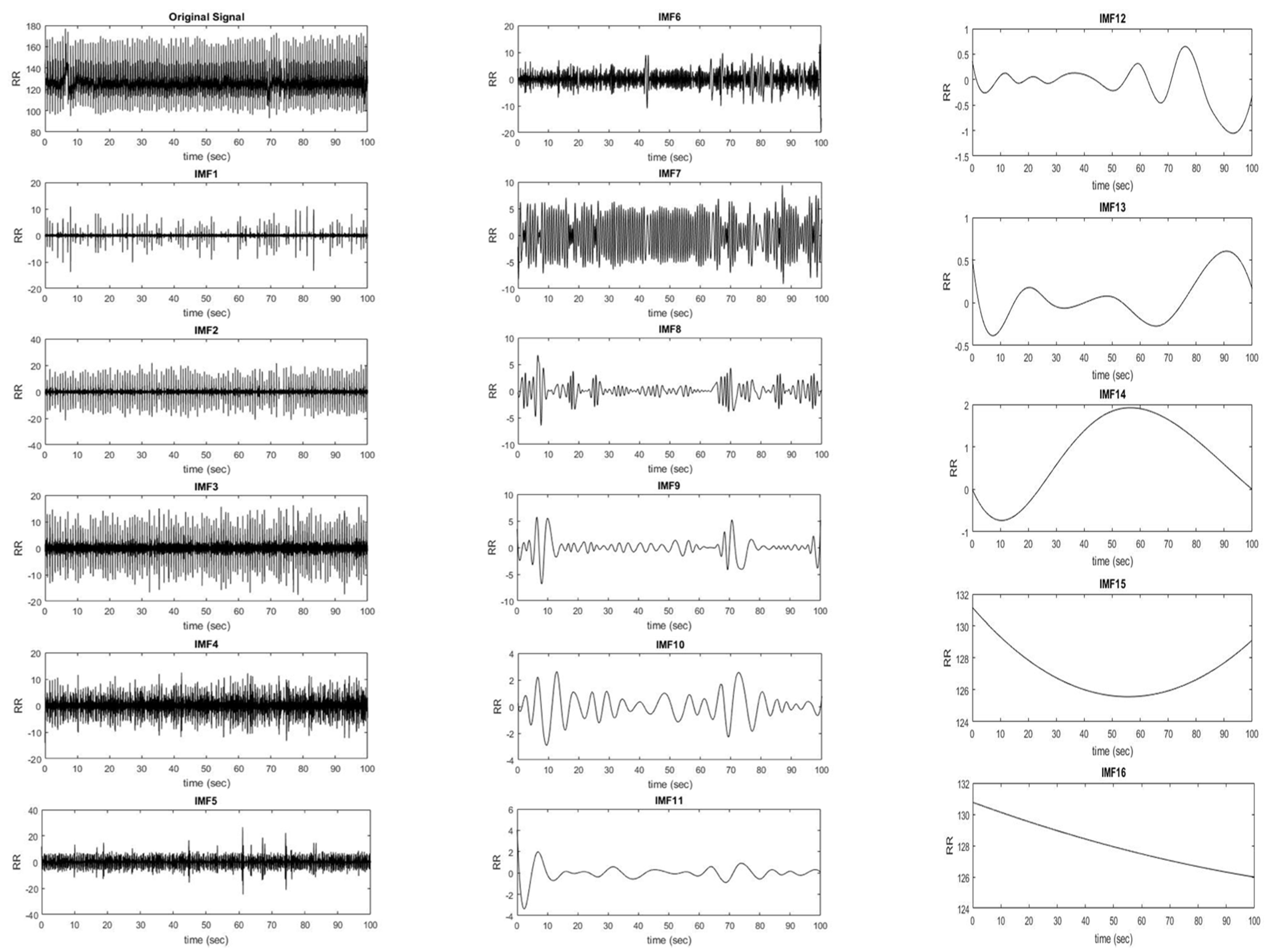
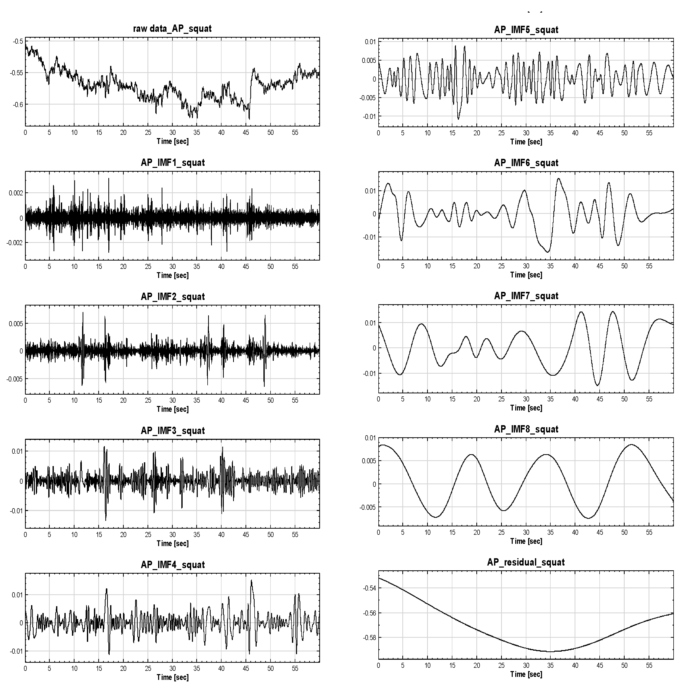
2.1. Decomposition of Sound Frequency Signals
- Determine the partial maxima and minima of the original signal . Then, use a cubic spline to connect the maxima to form an envelope and connect the minima to form another envelope. Aggregate and average the two envelopes to obtain the mean envelope . Subtract from to obtain the vector :
- Check if meets the constraints for the IMFs. If it does, return to Step (1), and take as the original signal for the second sifting process to obtain :
- After the sifting process is repeated k times, the original signal meets the constraints and becomes the IMF vector :
- Excessive sifting eliminates the original physical meaning. Hence, the following conditions are set for convergence to ensure that the IMFs maintain the original vibration amplitude and physical meaning:
- The number of zero-crossing points must be equal to that of the partial extrema (i.e., the partial maxima and partial minima), and the standard deviation (SD) should be between 0.2 and 0.3:
- If one of the conditions is met, the sifting process is complete, and the first IMF vector is obtained. is the shortest cycle of the entire set of signals:
- Subtract from to obtain the complementary function :
- If contains a longer cycle vector, repeat steps 1–5 to continue sifting and decompose it into n (cardinal number) IMF vectors :
- If cannot be decomposed into IMF vectors, the sifting process is suspended. The final is the mean trend. All IMF vectors are aggregated with the mean trend to obtain the original signal . Combine Equations (6) and (7) to obtain
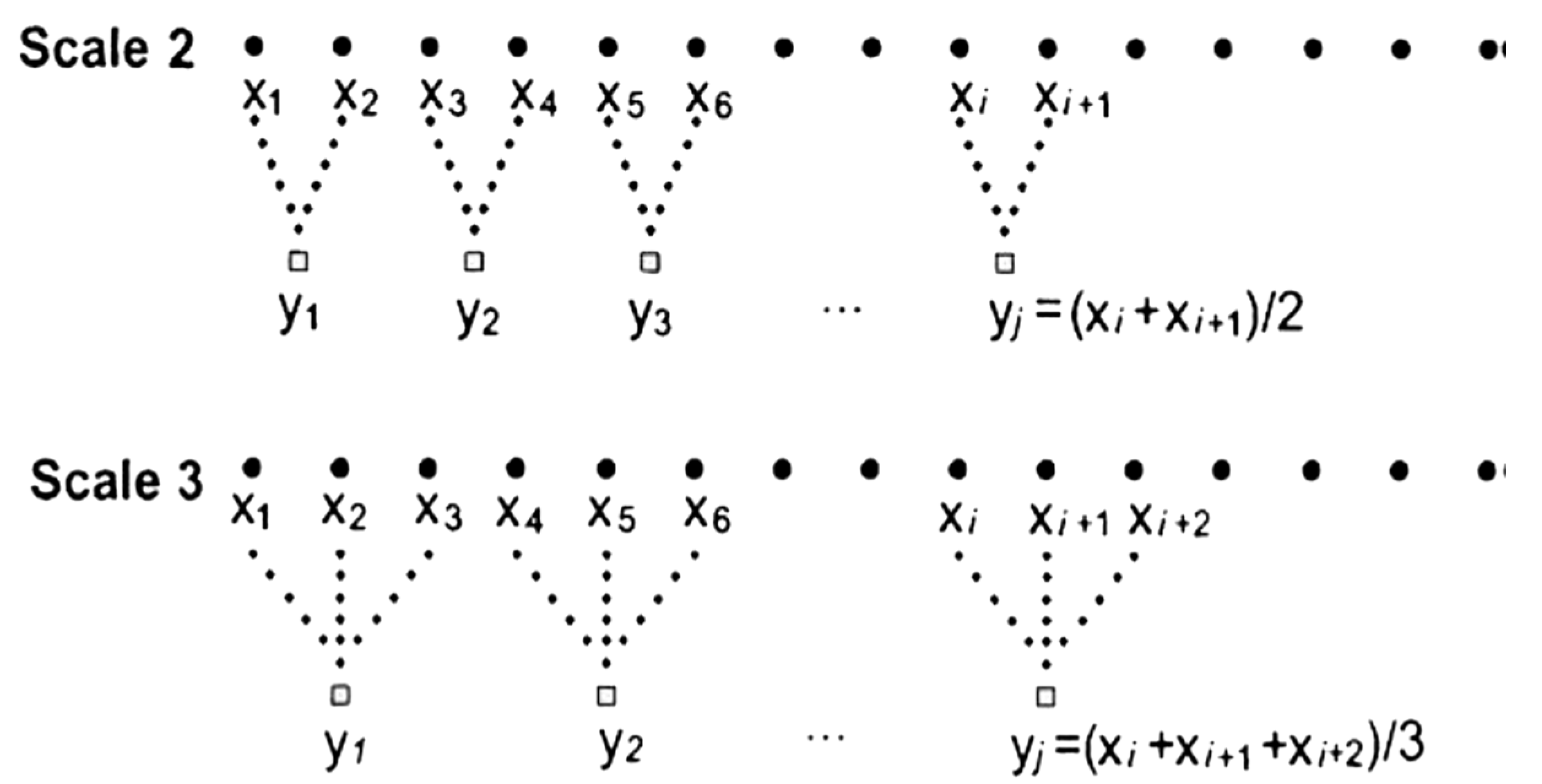
2.2. Recombination and Monitoring of Signals
2.3. Apply Hotelling T2 and Linear Discriminant Analysis to Sound Frequency Monitoring
2.4. Validation
2.4.1. Case Study I: Simulation Experiment
2.4.2. Case Study II: Electrocardiography Data
3. Results and Discussion
3.1. Case Study I
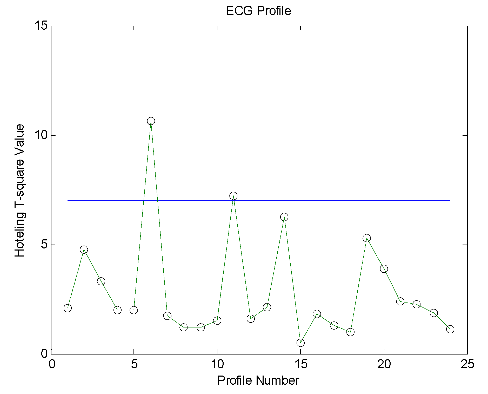
3.2. Case Study II
4. Conclusions
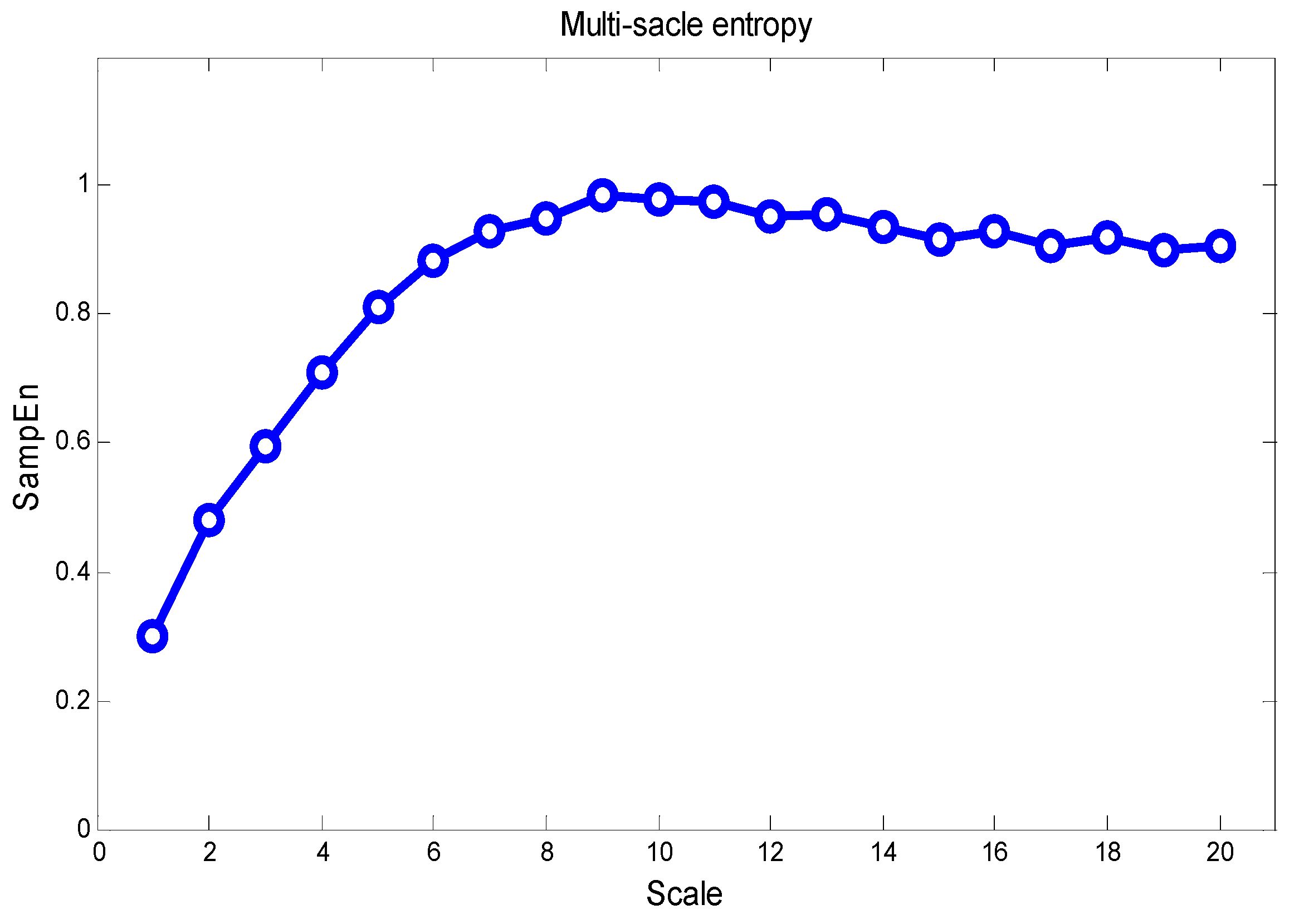
- The sound and vibration frequency signals were complex and unstable, but EMD removed unexpected signals and detected abnormal ones. Even when abnormal frequencies were placed at different time points, EMD was more effective than directly converting the original signal into an MSE profile. This demonstrates that monitoring a specific sound frequency indeed improves the identification of abnormal sound frequencies. The proposed method could also be applied to ECG signals.
- Good model fitting was obtained by converting the MSE profile into a fourth-order polynomial model. Although a complex model has a better fit than the third-order polynomial model, the latter is still advantageous owing to its fewer parameters and highly accessible LDA classification structure.
Author Contributions
Funding
Institutional Review Board Statement
Informed Consent Statement
Data Availability Statement
Conflicts of Interest
References
- Dai, X.W.; Gao, Z.W. From model, signal to knowledge: A data-driven perspective of fault detection and diagnosis. IEEE Trans. Ind. Inform. 2013, 9, 2226–2238. [Google Scholar] [CrossRef] [Green Version]
- Yan, K.; Ji, Z.; Shen, W. Online fault detection methods for chillers combining extended kalman filter and recursive one-class SVM. Neurocomputing 2017, 228, 205–212. [Google Scholar] [CrossRef] [Green Version]
- Sun, K.Z.; Li, G.N.; Chen, H.X.; Liu, J.Y.; Li, J.; Hu, W.J. A novel efficient SVM-based fault diagnosis method for multi-split air conditioning system’s refrigerant charge fault amount. Appl. Therm. Eng. 2016, 108, 989–998. [Google Scholar] [CrossRef]
- Rogers, A.P.; Guo, F.; Rasmussen, B.P. A review of fault detection and diagnosis methods for residential air conditioning systems. Build. Environ. 2019, 161, 106236. [Google Scholar] [CrossRef]
- Gangsar, P.; Tiwari, R. Signal based condition monitoring techniques for fault detection and diagnosis of induction motors: A state-of-the-art review. Mech. Syst. Signal Process. 2020, 144, 106908. [Google Scholar] [CrossRef]
- Neupane, D.; Seok, J. Bearing fault detection and diagnosis using Case Western Reserve University dataset with deep learning approaches: A review. IEEE Access 2020, 8, 93155–93178. [Google Scholar] [CrossRef]
- Fan SK, S.; Hsu, C.Y.; Jen, C.H.; Chen, K.L.; Juan, L.T. Defective wafer detection using a denoising autoencoder for semiconductor manufacturing processes. Adv. Eng. Inform. 2020, 46, 101166. [Google Scholar] [CrossRef]
- Fan SK, S.; Tsai, D.M.; He, F.; Huang, J.Y.; Jen, C.H. Key parameter identification and defective wafer detection of semiconductor manufacturing processes using image processing techniques. IEEE Trans. Semicond. Manuf. 2019, 32, 544–552. [Google Scholar] [CrossRef]
- Shao, X.; Barker, J. Stream weight estimation for multistream audio–visual speech recognition in a multispeaker environment. Speech Commun. 2008, 50, 337–353. [Google Scholar] [CrossRef] [Green Version]
- Xie, C.; Cao, X.; He, L. Algorithm of abnormal audio recognition based on improved MFCC. Procedia Eng. 2012, 29, 731–737. [Google Scholar] [CrossRef] [Green Version]
- Nalini, S.A.; Yusuf, D.J.; Alan Mackinnon, B. Application of acoustic directional data for audio event recognition via HMM/CRF in perimeter surveillance systems. Robot. Auton. Syst. 2015, 72, 15–28. [Google Scholar]
- Nalini, N.J. Music emotion recognition: The combined evidence of mfcc and residual phase. Egypt. Inform. J. 2016, 17, 1–10. [Google Scholar] [CrossRef] [Green Version]
- Lee, Y.C.; Shariatfar, M.; Rashidi, A.; Lee, H.W. Evidence-driven sound detection for prenotification and identification of construction safety hazards and accidents. Autom. Constr. 2020, 113, 103127. [Google Scholar] [CrossRef]
- Liu, Z.; Li, S. A sound monitoring system for prevention of underground pipeline damage caused by construction. Autom. Constr. 2020, 113, 103125. [Google Scholar] [CrossRef]
- Wei, J.; Wang, Z.; Xing, X. A Wireless High-Sensitivity Fetal Heart Sound Monitoring System. Sensors 2021, 21, 193. [Google Scholar] [CrossRef]
- Huang, N.E.; Shen, Z.; Long, S.R.; Wu, M.C.; Shih, H.H.; Zheng, Q.; Yen, N.C.; Tung, C.C.; Liu, H.H. The empirical mode decomposition and the Hilbert spectrum for nonlinear and non-stationary time series analysis. Proc. R. Soc. Lond. 1998, 454, 903–995. [Google Scholar] [CrossRef]
- Pachori, R.B.; Avinash, P.; Shashank, K.; Sharma, R.; Acharya, U.R. Application of empirical mode decomposition for analysis of normal and diabetic RR-interval signals. Expert Syst. Appl. 2015, 42, 4567–4581. [Google Scholar] [CrossRef]
- Safi, K.; Mohammed, S.; Albertsen, I.M.; Delechelle, E.; Amirat, Y.; Khalil, M.; Gracies, J.M.; Hutin, E. Automatic analysis of human posture equilibrium using empirical mode decomposition. Signal Image Video Process. 2017, 11, 1081–1088. [Google Scholar] [CrossRef]
- Alickovic, E.; Kevric, J.; Subasi, A. Performance evaluation of empirical mode decomposition, discrete wavelet transform, and wavelet packed decomposition for automated epileptic seizure detection and prediction. Biomed. Signal Process. Control 2018, 39, 94–102. [Google Scholar] [CrossRef]
- Wang, C.C.; Jiang, B.C.; Huang, P.M. The relationship between postural stability and lower-limb muscle activity using an entropy-based similarity index. Entropy 2018, 20, 320. [Google Scholar] [CrossRef] [Green Version]
- Wang, C.C.; Jiang, B.C.; Lin, W.C. Evaluation of effects of balance training from using wobble board-based exergaming system by MSE and MMSE techniques. J. Ambient. Intell. Humaniz. Comput. 2018, 9, 1745–1754. [Google Scholar] [CrossRef]
- Costa, M.; Goldberger, A.L.; Peng, C.K. Multiscale entropy analysis of biological signals. Phys. Rev. E 2005, 71, 021906-1–021906-18. [Google Scholar] [CrossRef] [PubMed] [Green Version]
- Riaz, M.; Saeed, U.; Mahmood, T.; Abbas, N.; Abbasi, S.A. An improved control chart for monitoring linear profiles and its application in thermal conductivity. IEEE Access 2020, 8, 120679–120693. [Google Scholar] [CrossRef]
- Fu, R.; Tian, Y.; Bao, T.; Meng, Z.; Shi, P. Improvement motor imagery EEG classification based on regularized linear discriminant analysis. J. Med. Syst. 2019, 43, 169. [Google Scholar] [CrossRef] [PubMed]


| 3-order polynomial model | 0.9241 |
| 4-order polynomial model | 0.9603 |
| 5-order polynomial model | 0.9594 |
| 1-sine model | 0.8513 |
| 2-sine model | 0.9214 |
| 3-sine model | 0.9011 |
| Three-sectioned 2-stage polynomial model | 0.9712 |
| Different Types of Abnormal Sound Frequency | Transforming Pattern | Accuracy |
|---|---|---|
| Abnormal sound for high frequency | Construct the profile to use EMD procedure via the LDA classification of high frequency | 96.28% |
| Construct the profile to use original signal via the LDA classification of high frequency | Unidentifiable | |
| Abnormal sound for intermediate frequency | Construct the profile to use EMD procedure via the LDA classification of intermediate frequency | 94.48% |
| Construct the profile to use original signal via the LDA classification of intermediate frequency | Unidentifiable | |
| Abnormal sound for low frequency | Construct the profile to use EMD procedure via the LDA classification of low frequency | 95.15% |
| Construct the profile to use original signal via the LDA classification of low frequency | Unidentifiable |
| Sample | 1 | 2 | 3 | 4 | 5 | 6 | 7 | 8 | 9 | 10 |
| 0.9902 | 0.9886 | 0.9903 | 0.9910 | 0.9874 | 0.9897 | 0.9911 | 0.9901 | 0.9788 | 0.9888 | |
| 0.9872 | 0.9813 | 0.9869 | 0.9896 | 0.9813 | 0.9815 | 0.9897 | 0.9899 | 0.9704 | 0.9817 | |
| Sample | 11 | 12 | 13 | 14 | 15 | 16 | 17 | 18 | 19 | 20 |
| 0.9909 | 0.9910 | 0.9913 | 0.9874 | 0.9901 | 0.9895 | 0.9899 | 0.9885 | 0.9913 | 0.9905 | |
| 0.9889 | 0.9887 | 0.9896 | 0.9827 | 0.9891 | 0.9808 | 0.9832 | 0.9803 | 0.9881 | 0.9843 | |
| Sample | 21 | 22 | 23 | 24 | ||||||
| 0.9889 | 0.990 | 0.9876 | 0.9914 | |||||||
| 0.9834 | 0.9811 | 0.9809 | 0.9897 |
| Type of Signals | Profile Transformation | Accuracy Rate |
|---|---|---|
| Normal ECG signals | Profile transformation using EMD | 97.92% |
| Profile transformation using original signal | 71.42% | |
| Irregular heartbeat | Profile transformation using EMD | 92.20% |
| Profile transformation using original signal | 65.52% |
Publisher’s Note: MDPI stays neutral with regard to jurisdictional claims in published maps and institutional affiliations. |
© 2021 by the authors. Licensee MDPI, Basel, Switzerland. This article is an open access article distributed under the terms and conditions of the Creative Commons Attribution (CC BY) license (https://creativecommons.org/licenses/by/4.0/).
Share and Cite
Jen, C.-H.; Wang, C.-C. Real-Time Process Monitoring Based on Multivariate Control Chart for Anomalies Driven by Frequency Signal via Sound and Electrocardiography Cases. Processes 2021, 9, 1510. https://doi.org/10.3390/pr9091510
Jen C-H, Wang C-C. Real-Time Process Monitoring Based on Multivariate Control Chart for Anomalies Driven by Frequency Signal via Sound and Electrocardiography Cases. Processes. 2021; 9(9):1510. https://doi.org/10.3390/pr9091510
Chicago/Turabian StyleJen, Chih-Hung, and Chien-Chih Wang. 2021. "Real-Time Process Monitoring Based on Multivariate Control Chart for Anomalies Driven by Frequency Signal via Sound and Electrocardiography Cases" Processes 9, no. 9: 1510. https://doi.org/10.3390/pr9091510
APA StyleJen, C.-H., & Wang, C.-C. (2021). Real-Time Process Monitoring Based on Multivariate Control Chart for Anomalies Driven by Frequency Signal via Sound and Electrocardiography Cases. Processes, 9(9), 1510. https://doi.org/10.3390/pr9091510