End-to-End Control Chart Pattern Classification Using a 1D Convolutional Neural Network and Transfer Learning

Abstract

Control charts are an important tool in statistical process control (SPC). They have been commonly used for monitoring process variation in many industries. Recognition of non-random patterns is an important task in SPC. The presence of non-random patterns implies that a process is affected by certain assignable causes, and some corrective actions should be taken. In recent years, a great deal of research has been devoted to the application of machine learning (ML) based approaches to control chart pattern recognition (CCPR). However, there are some gaps that hinder the application of the CCPR methods in practice. In this study, we applied a control chart pattern recognition method based on an end-to-end one-dimensional convolutional neural network (1D CNN) model. We proposed some methods to generate datasets with high intra-class diversity aiming to create a robust classification model. To address the data scarcity issue, some data augmentation operations suitable for CCPR were proposed. This study also investigated the usefulness of transfer learning techniques for the CCPR task. The pre-trained model using normally distributed data was used as a starting point and fine-tuned on the unknown non-normal data. The performance of the proposed approach was evaluated by real-world data and simulation experiments. Experimental results indicate that our proposed method outperforms the traditional machine learning methods and could be a promising tool to effectively classify control chart patterns. The results and findings of this study are crucial for the further realization of smart statistical process control.

1. Introduction

Control charts are an important tool in statistical process control (SPC) used to determine if a manufacturing or business process is in a state of statistical control. When a non-random pattern appears in the control chart, it means that one or more assignable causes which will gradually degrade the process quality exist. The importance of non-random pattern lies in the fact that it can provide relevant information about process diagnosis. Montgomery [1] pointed out that every non-random pattern can be mapped to a set of assignable causes. Therefore, if the pattern type can be correctly recognized and identified, it will help to diagnose the possible causes of the manufacturing process problem. Some real-world examples that used non-random patterns to identify potential causes can be found in [2,3].

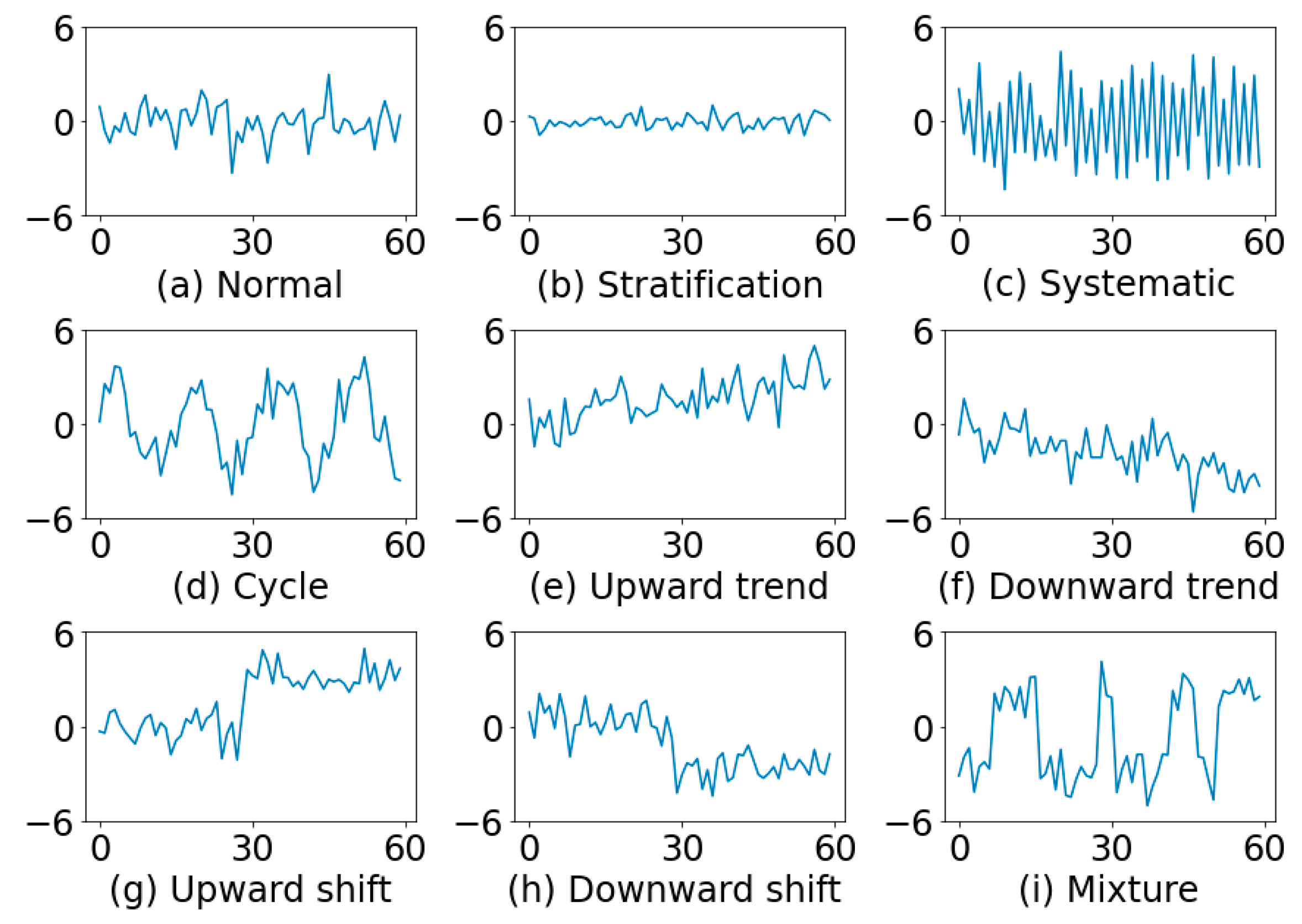
Western Electric Company [4] first identified various types of non-random patterns and developed a set of sensitizing rules for analysis. Nelson [5,6] further established a set of run rules for non-random patterns. Figure 1 illustrates some typical examples of control chart patterns. A normal pattern (NOR) will exhibit only random variations (Figure 1a). In stratification (STRA), there is a lack of natural variability, the points tend to cluster around the center line (Figure 1b). In systematic variations (SYS), a high point is always followed by a low one, or vice versa (Figure 1c). A cycle (CYC) can be recognized by a series of high portions or peaks interspersed with low portions or troughs (Figure 1d). A trend can be defined as a continuous movement in one direction. Figure 1e shows an upward trend (UT) and Figure 1f a downward trend (DT). A shift may be defined as a sudden or abrupt change in the average of the process. Figure 1g indicates an upward shift (US) and Figure 1h a downward shift (DS). In a mixture (MIX) pattern, the points tend to fall near the high and low edge of the pattern with an absence of normal fluctuations near the middle (Figure 1i). A mixture can be thought of as a combination of data from separate distributions.

Although supplementary rules [4,5,6] are useful in identifying the out-of-control situations, Cheng [7] pointed out that there is no one-to-one mapping between a supplementary rule and a non-random pattern. It is worth noting here that the control chart pattern recognition task has its own unique challenges and difficulties, such as high intra-class variability (due to different magnitudes and translation of the pattern) and high inter-class similarity (due to the preceding in-control data and some resemblance between patterns). All these challenges make it highly desirable to develop an intelligent-based approach to effectively classify the non-random control chart patterns.

In recent years, a great deal of research has been devoted to the application of machine learning (ML)-based approaches to control chart pattern recognition (CCPR) with the purposes of improving the classification performance and serving as a supplementary tool to traditional control charts [8]. It is anticipated that the ML-based classification models can replicate engineers’ analysis mechanisms. With the development of the Industrial Internet of Things (IIOT) and artificial intelligence (AI), it has become increasingly feasible to collect process data and use intelligent decision-making models for analysis. The intelligent-based detection and diagnosis system is more important than ever before [9]. Hachicha and Ghorbel [10] conducted a comprehensive review of recent research on control chart pattern recognition. The classification approaches include rule-based [11,12], decision tree (DT) [13,14], artificial neural network (ANN) [7,15,16], support vector machine (SVM) [17,18]. Previous studies focused on the recognition of basic non-random patterns. Some studies [16,18,19,20] have conducted research on the recognition of concurrent patterns (the combination of two or more basic patterns simultaneously).

In previous studies, the input vector of the classification model can be raw data [7,15] or hand-crafted features [13,14,21,22,23]. When taking raw data as inputs, each observation is treated as an individual feature. The major drawback with ML algorithms like DT, ANN, and SVM is that these methods consider each input feature individually and do not consider the sequence which these features follow. In other words, different orders of the same features are treated as the same inputs. However, in SPC application, the input features are observations which follow a sequence that characterizes the specific pattern class. The classification approach may be sensitive to the location in time of the discriminative features.

In addition to raw data-based models, feature-based methods have also been widely used in control chart pattern recognition, they are heuristic and highly depend on human experts. The features from feature extraction carry information of the time series, which is not based on individual time points, they are less sensitive to the variation of control chart pattern. Nevertheless, the feature-based approach is not without its problems and limitations. In traditional approaches, features were heuristically engineered based on prior knowledge about non-random patterns. However, the patterns that appeared in the analysis window were too simple. Excepting shift patterns, the starting point for other non-random patterns was often assumed to be the first observation in the window. The hand-crafted features for this kind of pattern behavior may not be applicable to other variants of patterns. In addition, the existing feature-based machine learning methods utilize expert knowledge to extract features, which is both time consuming and error-prone. The feature extraction method may have signal loss and does not describe the characteristics of control chart patterns well. The problem would become more severe when considering the variants of non-random patterns.

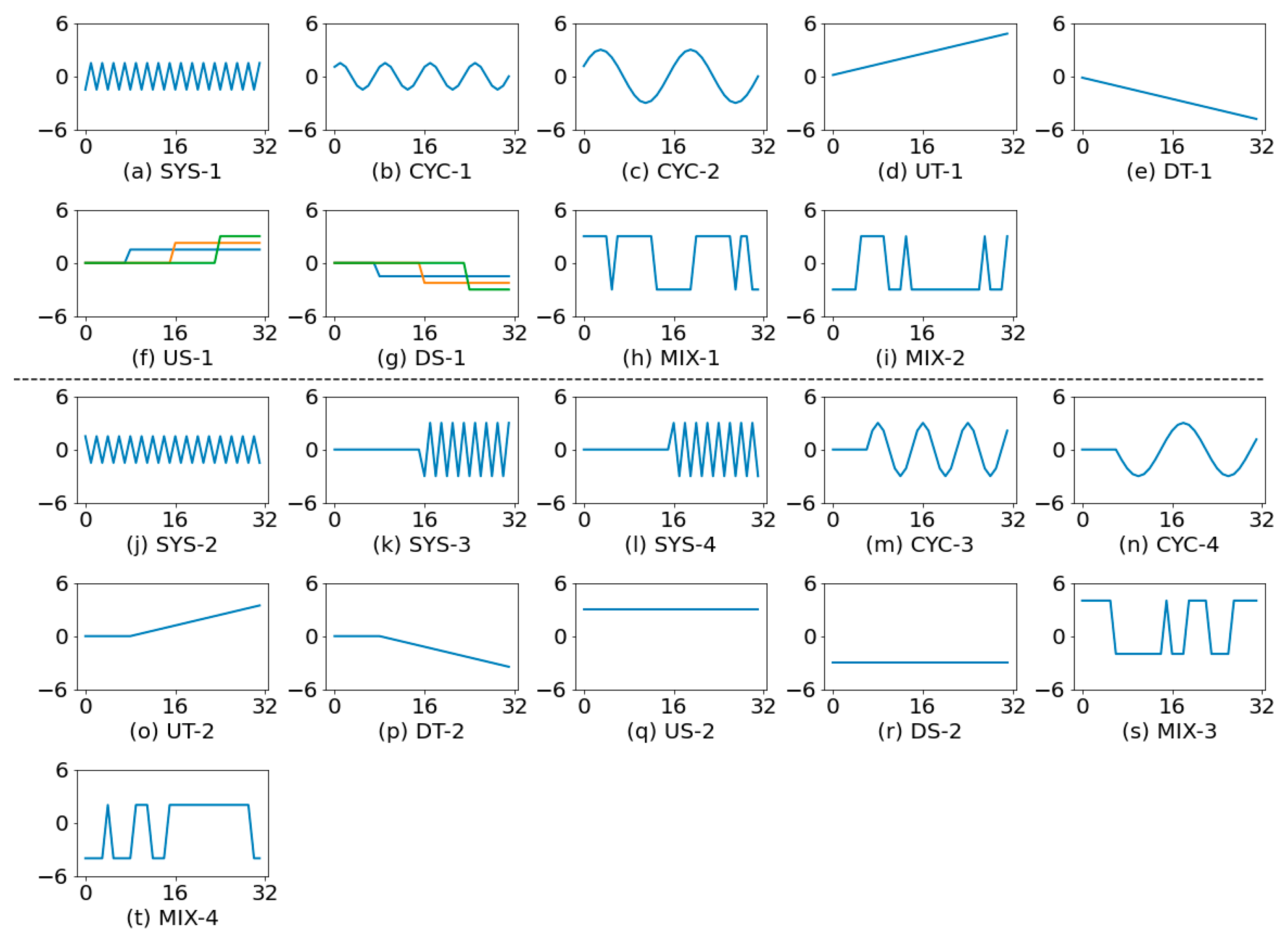
Here, we would like to emphasize the important concept of translation invariance [24,25]. The CCPR is often implemented in an analysis window approach. The observed values at multiple time steps are grouped to form an input vector for a classification model. The width of the analysis window (i.e., the number of consecutive observations) can be varied to include more or less previous time steps, depending on the complexity of the problem. Most previous studies overlooked the importance of translation invariance property of CCPR classifiers. When the window moves over the time, one may see different variants of a specific type of pattern (see Figure 2). For CCPR, the translational invariance means that the classifier would recognize the pattern regardless of where it appears in the window.

One critical issue needs to be addressed in ML-based CCPR is the scarcity of data. Previous research often relied on simulations to generate training and test data since field data collection can be expensive, time consuming, and difficult [10,21]. This approach is acceptable if the underlying distribution is known or can be correctly identified. However, a high diversity in the training data is still required so that the classification model becomes robust to intra-class variability. As discussed above, the analysis window may produce many variants of a pattern when it slides along the time series data.

Apart from the above issues, some researchers have commented on the practical application of CCPR. Woodall and Montgomery [26] stated that machine learning-based CCPR methods do not have a practical impact on SPC. Weese et al. [27] further pointed out some gaps that hinder the application of the CCPR methods in practice. They recommended some research directions in the practical application of CCPR methods, including the robustness of CCPR methods to the baseline training sample size, the selection of CCPR structures, etc.

For a long time, researchers have focused on using advanced methods to improve the classification accuracy of CCPR. Recently, the application of deep learning to CCPR has been investigated. Hong et al. [28] applied a convolutional neural network (CNN) to the concurrent pattern recognition problem. Miao and Yang [29] selected statistical and shape features used them to train a CNN. They addressed concurrent CCPR problems. Xu et al. [30] developed a 1D CNN for recognition of control chart patterns. They showed that CNN was robust to the deviation between the distribution of test data and training data. Yu et al. [31] presented a deep learning method known as stacked denoising autoencoder for CCPR feature learning. Chu et al. [32] proposed a data enhancement method to improve the performance of the deep belief network in CCPR. Fuqua and Razzaghi [33] designed a CNN to address the imbalanced CCPR problem. Most recently, Zan et al. [8] applied a 1D CNN to CCPR. They demonstrated the benefits of CNN using simulated data and a real-world dataset. Zan et al. [34] proposed a method based on multilayer bidirectional long short-term memory network (Bi-LSTM) to learn the features from the raw data. Using a simulation study, they demonstrated that Bi-LSTM performed better than other methods including 1D CNN.

A review of previous studies indicates that there are research gaps in the literature. First, the variations of non-random patterns used to evaluate the CCPR performance are oversimplified. After surveying more than 120 papers published on CCPR studies, Hachicha and Ghorbel [10] criticized the fact that past research trained the model in a static mode without considering the dynamic nature of the non-random patterns. They further pointed out that future work should address the problem of the misalignment of the pattern in time. Zan et al. [8] pointed out the importance of increasing the variability of training dataset. They suggested that training patterns should be carefully prepared to ensure the closeness to the real patterns. The above arguments indicate the needs of creating a diversified dataset in order to enhance the robustness of the CCPR model the dynamic nature of non-random patterns.

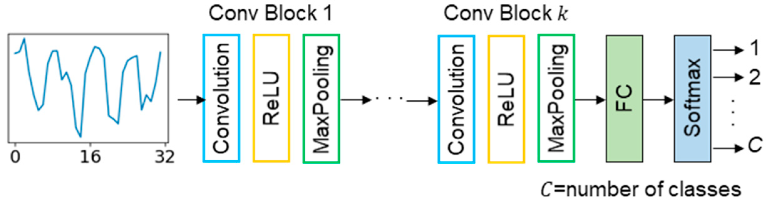
To address the aforementioned issues, we propose a control chart pattern recognition method based on an end-to-end one-dimensional convolutional neural network model (1D CNN) architecture. CNN is a deep learning neural network algorithm, most commonly applied to computer vision [35,36,37]. Recently, researchers have demonstrated that it is possible to apply CNN not only to image recognition tasks but also to time series classification tasks [38,39]. The main advantage of CNN is that it automatically learns the important features without any hand-crafted feature extraction. The end-to-end classification system performs feature extraction jointly with classification. More importantly, CNN is capable to learn the translation invariance features from the input.

If patterns can be generated by simulation, we proposed a flexible method to generate dataset with high intra-class diversity. When patterns cannot be generated by explicit formulas, some data augmentation operations suitable for CCPR are proposed and investigated. With the purpose to deal with data scarcity and long model training rime, we also examined the application of transfer learning to CCPR. A pre-trained model based on frequently encountered data, can be applied to other unknown data types with minor retrain. The major contributions of this work are summarized as follows:

• We propose a new pattern generator to produce high diversity in the dataset so that the classification model becomes robust to the dynamic nature of the non-random patterns.
• We propose an end-to-end classification model based on 1D CNN architecture to classify control chart patterns directly without preprocessing or feature engineering. We conduct a thorough comparison with other feature-based approaches, including time-domain and frequency-domain features. Through exhaustive evaluation, we prove our method achieves better classification accuracy than the existing ML-based methods.
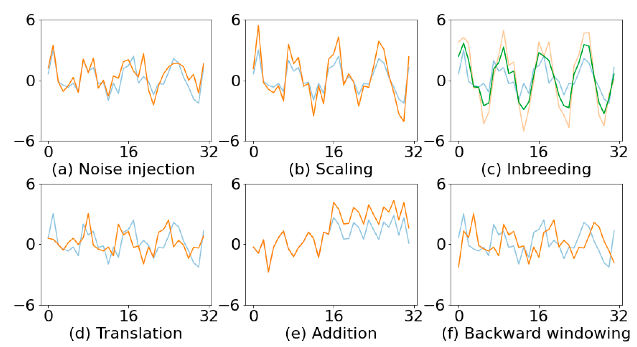
• We present some data augmentation methods for control chart patterns and perform an analysis of the effects of data augmentation on classification accuracy.
• We explore the application of transfer learning to CCPR by investigating if CNN trained on normally distributed data can still perform well for any continuous distribution data.

The rest of the paper is organized as follows. Section 2 first describes the architecture of 1D CNN for classification and the concepts of transfer learning, and then the brief introduction of traditional classification models relevant to this research. Section 3 presents the proposed methods, including pattern generation, data augmentation methods and the proposed 1D CNN for control chart pattern recognition. Section 4 presents the performance evaluation results for the 1D CNN and other methods using different datasets, including real-world data, publicly available dataset, and simulated dataset. This section also provides the results of using different transfer learning approaches. Section 5 summarizes the contributions of this study and provides remarks on limitations and future research directions.

2. Theoretical Background

The following subsections describe the basic concepts of 1D CNN for classification, transfer learning and various classification models relevant to this research.

2.1. 1D CNN for Classification

A 1D CNN usually includes one or more convolution layers, activation layers, pooling layers and fully connected layers [38]. Convolution and pooling layers perform feature extraction, whereas the fully connected layers accomplish classification. The convolution layer is called feature map and sometimes a feature detector. A pooling layer will perform a subsampling function using the inputs it received from the previous convolution layer. The combination of convolution layer, activation layer, and pooling layer is usually referred to as a convolution block (Conv Block). In this study, rectified linear unit (ReLU) was selected as the activation function. At the end of the network, fully connected layers will be added. They work as a classification module for the network. The output layer is composed of $C$ units for a classification task with $C$ classes. A typical architecture is depicted in Figure 3.

In the Conv Block, the 1D convolution layer is used to extract feature maps and different numbers of 1D convolution filters of the same size are applied in each layer. As the Conv Block goes deeper, the number of convolutional filters is increased (doubling the number of filters every block). The amount of movement between applications of the filter (refers to as stride) is usually set to one.

The role of pooling is used to reduce the number of dimensions in the feature maps and network parameters. Using a pooling layer and creating pooled feature maps can obtain a summarized version of the features detected in the input. Max pooling with the size of 2 is the most commonly used pooling strategy. The pooling layer will reduce the size of each feature map by a factor of 2. Pooling leads to an important characteristic called the model’s invariance to local translation. Invariance to translation means that if the input is translated by a small amount, the values of most of the pooled outputs will not change. This characteristic is extremely important for CCPR since it may encounter many variants of the original pattern.

The output from the final pooling or convolution layer will be flattened and then fed into one or more fully connected (FC) layers. The fully connected layers use the features learned from convolution operations to perform the classification task. The number of neurons in a fully connected layer is usually determined by experimentation. The final output layer of the network is a softmax classifier, which has the same number of outputs as the number of classes. The softmax function normalizes output values from the last fully connected layer to target class probabilities, where each value ranges between 0 and 1 and all values sum to 1. The softmax function can be written as:

$$f\left(z_i\right)=\left(\frac{e^{z_i}}{{{\displaystyle \sum }}_{j=1}^C{e}^{z_j}}\right)$$

(1)

where $z$ is the activation value of last layer of neurons. The activation value of neuron $i$ is $z_i$. The class label of the maximum probability is chosen as the output; therefore, the label of the predicted class $\widehat{y}$ is determined as follows:

$$\widehat{y}=\arg \underset{i}{\max }\left(f\left(z_i\right)\right)$$

(2)

where $C$ is the number of classes and the number of last layer neurons. Classification loss is calculated by comparing the class probabilities ($p_i$) and true labels of samples ($y_i$). The loss can be calculated as follows:

$$\mathrm{Loss}=-{{\displaystyle \sum }}_{i=1}^C{y}_i\log \left(p_i\right)$$

(3)

The loss can be minimized using an optimization algorithm which iteratively updates the learnable parameters in the network. Commonly used methods include stochastic gradient descent (SGD), RMSprop (root mean square prop) and Adam (adaptive moment estimation) [40].

2.2. Traditional Classification Models

2.2.1. Support Vector Machines

Support vector machines (SVMs) are a set of supervised learning methods used for classification (SVC), regression (SVR) and outlier detection [41]. SVC was first designed for binary classification. It can be adapted to multi-class classification problem using the one-vs.-one or one-vs.-rest method [42]. One-vs.-rest is a heuristic method for using binary classification algorithms for multi-class classification. It involves splitting the multi-class dataset into multiple binary classification problems. The one-vs.-one strategy splits a multi-class classification into one binary classification problem per each pair of classes. To optimize the classification performance, the SVC classifier parameters, kernel width $\gamma$ and regularization constant $C$, must be chosen effectively.

2.2.2. Random Forest

Random forest (RF) is an ensemble machine learning algorithm and can be used for classification and regression problems [43]. Random forest involves constructing a large number of decision trees using bootstrap samples from the training dataset. Random forest also involves selecting a subset of input features at each split point in the construction of trees. For regression problems, prediction is the average prediction across the decision trees. A prediction on a classification problem is the majority vote for the class label across the trees in the ensemble.

The most important hyperparameter to tune for the random forest is the number of random features to consider at each split point. In the regression context, Breiman [43] recommends setting the number of random features to be one-third of the number of predictors. For classification problems, Breiman [43] recommends setting this hyperparameter to the square root of the number of features. The number of trees is another key hyperparameter to configure for the random forest. Typically, the number of trees is increased until the model performance stabilizes. A final important hyperparameter is the maximum depth of decision trees used in the ensemble. Greater depth of the trees often leads to higher accuracy, but also increases the chances overfitting.

2.2.3. Time Series Forest

Deng et al. [44] proposed a time series forest (TSF) algorithm for time series classification. Training a single tree involves selecting $\sqrt{m}$ random intervals for each series, where $m$ is the length of time series data. Summary statistics including the mean, standard deviation and slope of the interval were calculated as features. Each tree will use $3\sqrt{m}$ features as input data. Classification result is based on a majority vote of all the trees in the ensemble. The influential parameters of this algorithm include the number of trees in the forest and the minimum length of the intervals.

2.3. Transfer Learning

Deep learning has shown noteworthy success in many application areas. However, a large amount of labeled training data is often required when building a deep learning model from scratch. This is one of the issues that has led to the development of the research field of transfer learning (TL) [45,46]. Transfer learning involves using a pre-trained model on one problem (source task, where a large amount of data is available) as a starting point and then applying it to a related problem (target task). Transfer learning is considered as a method to compensate for the lack of sufficient training data. In addition, transfer learning has the benefit of decreasing the training time for a deep learning model and can result in lower generalization error.

In the following, we use CNN as the example to illustrate the usages of a pre-trained model. A typical CNN comprises a convolutional base and a classifier. Convolutional base consists of a stack of convolutional and pooling layers. The classifier in CNN is usually composed of fully connected layers. There are many ways to apply the pre-trained model depending on the similarity between source domain and target domain as well as the availability of training data. Figure 4 illustrates some simple usage of pre-trained models. In the first strategy, the pre-trained model is used as-is to classify new inputs. In the second approach, the pre-trained model is used as a feature extractor to extract relevant features. In this approach, we freeze the weights of the convolutional base and then train the network to update the weights of the new fully connected layers. This approach is appropriate when the target dataset is small and similar to the source training dataset.

Fine-tuning a pre-trained network model on a new dataset is the most common transfer learning strategy in the context of deep learning. One approach is to fine-tune (train) the last few layers of the pre-trained model while freezing the parameters of the remaining initial layers to their pre-trained values. In this way, we reuse the initial (bottom) layers of CNN that preserve more abstract, generic features. On the other hand, we would like to fine-tune the layers toward the end (top) of a CNN, since they tend to provide more specific, task-related features. We can also initialize the new model with the parameters of the pre-trained model, and then optimize all the parameters of the CNN network using the target training data. This usage treats transfer learning as a type of weight initialization scheme. In [47] the authors referred to it as standard fine-tuning. This approach is appropriate when the size of target dataset is large otherwise it may result in overfitting. Some variants of fine-tuning can be found in [47,48].

3. Methodology

3.1. Generation of Patterns

Previous research often relied on the simulation to generate training and test data since field data collection can be expensive, time consuming, and difficult [13,14,21]. This approach is acceptable if the underlying distribution is known or can be correctly identified. However, a high diversity in the training data are required so that the classification model becomes robust to the intra-class variability. The analysis window may produce many variants of a pattern when it slides along the time series data. The problem is similar to the issue of misalignment of pattern in time raised by Hachicha and Ghorbel [10]. They argued that the CCPR model needs to identify a dynamic control chart pattern. One way to address this issue is to develop an adequate training dataset containing the variation of patterns that may encounter in the identification process. In this research, we propose some methods to generate datasets with high intra-class diversity.

For online and real time operation of CCPR, different variants of non-random patterns have to be considered. To account for the variants of a non-random pattern appeared in a sliding analysis window, a generalized pattern generator is proposed. Figure 5 illustrates the variants of each non-random pattern. In Figure 5, the subplots located above the dotted line represent the non-random patterns considered in most of the previous research [13,14,21]. Except for shift patterns, the change point is fixed at the first position in the analysis window. The models trained using this approach cannot be expected to perform well in classifying dynamic patterns. The subplots located below the dotted line are the additional non-random patterns investigated in the present study. Figure 5j–l represent different variants of systematic patterns. We allow the pattern to appear at any location in the window. The first point of the pattern can be located above or below the mean. For cyclic patterns (Figure 5m,n), they can be sine wave or cosine wave. In addition, the cycle may be preceded by some in-control data. For trends (Figure 5o,p), the starting point can be located at any position of the window. For shifts (Figure 5q,r), we consider the totally shifted data. For mixture pattern (Figure 5s,t), each group may have different shift magnitudes.

Here we describe the pattern generators modified from previous studies [13,21]. The major changes are taking the dynamic nature of the control chart patterns into consideration. Similar to the applications of previous studies [13,21], the proposed generators can be applied to an individual value or a sample mean. The observation at time $t$ can be written as $x_t=\mu +d_t+n_t$, where $\mu$ is the process mean when the process is in control, $d_t$ the disturbance term, and $n_t~N\left(0,{\sigma }^2\right)$ the noise term. Without loss of generality, we assume $\mu =0$ and $\sigma =1$. The observation is simplified to $x_t=d_t+n_t$, and $n_t~N\left(0,1\right)$. For normal pattern, $d_t=0$. The equations used to generate $d_t{}^{\prime }s$ for different non-random patterns are summarized as follows:

• Systematic

  $$d_t=\{\begin{array}{ll}0,\hfill & \mathrm{if}t<t_0\hfill \\ {\left(-1\right)}^{\left(t-t_0+t^{*}\right)}{\mathsf{\Delta }}_1,\hfill & \mathrm{if}t\ge t_0\hfill \end{array}$$

  (4)

  where $t_0$ is the starting point of systematic pattern; ${\mathsf{\Delta }}_1$ is the shift size of systematic pattern expressed in terms of $\sigma$. The quantity $t^{*}$ denotes a random integer value in the range [0,1]. It determines the location of the first observation.
• Cycle

  $$d_t=\{\begin{array}{ll}0,\hfill & \mathrm{if}t<t_0\hfill \\ \kappa \cdot \sin \left(2\pi \left(t-t_0+1\right)/\mathsf{\Omega }\right),\hfill & \mathrm{if}t\ge t_0\hfill \end{array}$$

  (5)

  where $t_0$ is the starting point of cycle; $\kappa$ is the amplitude of cycle expressed in terms of $\mathsf{\sigma }$.
• Upward trend or downward trend

  $$d_t=\{\begin{array}{ll}0,\hfill & \mathrm{if}t<t_0\hfill \\ \pm \theta \cdot \left(t-t_0+1\right),\hfill & \mathrm{if}t\ge t_0\hfill \end{array}$$

  (6)

  where $t_0$ is the starting point of trend; $\theta$ is slope of trend expressed in terms of $\sigma$. The sign of $\theta$determines the direction of trends.
• Upward shift or downward shift

  $$d_t=\{\begin{array}{ll}0,\hfill & \mathrm{if}t<t_0\hfill \\ \pm {\mathsf{\Delta }}_2,\hfill & \mathrm{if}t\ge t_0\hfill \end{array}$$

  (7)

  where $t_0$ is the starting point of the shift pattern; ${\mathsf{\Delta }}_2$ is the shift size expressed in terms of $\sigma$. The sign of ${\mathsf{\Delta }}_2$determines the direction of shifts.
• Mixture

  $$d_t=\{\begin{array}{ll}0,\hfill & \mathrm{if}t<t_0\hfill \\ {\mathsf{\Delta }}_3,\hfill & \mathrm{if}t\ge t_0 and \nu >P{r}_1\hfill \\ {\mathsf{\Delta }}_4,\hfill & \mathrm{if}t\ge t_0 and \nu <P{r}_1\hfill \end{array}$$

  (8)

  where $t_0$ is the starting point of mixture; ${\mathsf{\Delta }}_3$($>$0) and ${\mathsf{\Delta }}_4$($<$0) are the offsets from the mean expressed in terms of $\sigma$. The quantity $\nu$ denotes a random number ranging between 0 and 1. $P{r}_1$ is a probability controlling the position of the first shifted observation. For $t\ge t_0+1$, the $d_t$ is determined by the following rules:

  $$d_t=\{\begin{array}{ll}{d}_{t-1},\hfill & \mathrm{if}\nu >P{r}_2\hfill \\ {\mathsf{\Delta }}_4,\hfill & \mathrm{if}\nu <P{r}_2 and d_{t-1}>0\hfill \\ {\mathsf{\Delta }}_3,\hfill & \mathrm{if}\nu <P{r}_2 and d_{t-1}<0\hfill \end{array}$$

  (9)

  where $P{r}_2$ is the probability of shifting between distributions. A small value of $P{r}_2$ indicates a less tendency of changing distribution.

The equations for cycles, trends and shifts are similar to those used in previous studies [13,21]; however, we allow some in-control data to precede the non-random patterns. By changing the value of $t_0$, we can generate various variants of a specific pattern and address the dynamic nature of non-random patterns. In most of the previous studies, the quantity $t_0$was set to 1 with the exception of shift patterns. In generating shift patterns, $t_0$was usually set at around the middle of the analysis window in previous studies. It is worth noting that when $t_0=1$, the above equations are reduced to that used in previous studies [13,21].

3.2. Data Augmentation

In developing a control chart pattern classifier, sufficient data are required to build an efficient model. Unfortunately, due to the cost of data collection, a large number of sample patterns are not economically available. In addition, data with non-random pattern are rare events in most manufacturing processes. Therefore, most of the previous studies adopt the simulation approach to generate pattern data. Data augmentation is a technique that can be used to artificially expand the size of a training dataset by creating modified versions of data. Data augmentation helps to generate synthetic data from existing dataset such that generalization capability of model can be improved.

For image recognition applications, there are various techniques including mirroring, scaling, cropping, and rotating [24]. However, these methods do not generalize well to time series. Data augmentation methods for time series data can be found in [49,50,51,52]. However, in the case of CCPR the application of data augmentation has been relatively limited.

Previous studies indicated that different augmentation techniques have varying results for different datasets. This suggests that not all data augmentation techniques work equally well for all classification tasks, or for different datasets. The selection of data augmentation methods should be based on domain knowledge. We should confirm the effect of such transformations on the nature of pattern data.

In the present study, we proposed some data augmentation methods that can be used to synthetically generate pattern data in practical applications of control chart pattern recognition. The methods considered in this study include noise injection, scaling, inbreeding, pattern translation, addition/subtraction, and backward windowing. Noise injection [47,48,49] is a method which adds a small amount of noise into a time series without changing the corresponding class labels. White Gaussian noise or uniform noise could be added to raw training data. This method could be applied to any of the control chart patterns. Adding noise to time series can help a classification model learn more robust features and enhance generalization capability [23]. The effect of injecting noise on the dataset is illustrated in Figure 6a. Scaling [47,48,49] is implemented by multiplying the raw training data by a random scalar. Scaling can lead to different magnitudes of non-random patterns. This method could be applied to systematic patterns, cyclic patterns, and mixtures. Figure 6b shows an augmented cyclic pattern after applying scaling operation. The above methods are commonly used in the time series classification research [47,48,49] and we will not elaborate here. In the following, we describe our proposed methods suitable for use in CCPR.

1.

Inbreeding

We take two time series $x_i$ and$x_j$ that involve assignable cause(s) ($x_i$ and$x_j$ are in the same class) and do a linear combination of them: $x_{\mathrm{new}}=\alpha x_i+\left(1-\alpha \right)x_j$, where $\alpha$ is between 0 and 1. This method could be applied to any of the control chart patterns. Figure 6c shows an augmented cyclic pattern after applying inbreeding operation.

2.

Pattern translation

This method involves adding some in-control data in the front of time series $x_i$ that involves assignable cause(s). This method could be applied to any type of the non-random patterns. This method is equivalent to translating $x_i$ along the time. It is important to apply this translation since pattern can appear at any location in the window. Figure 6d shows an augmented cyclic pattern after applying translation operation.

3.

Addition and subtraction

The concept of this method is to add and subtract a certain amount to the time series $x_i$ that involves assignable cause(s). This method can be applied to shift patterns. Figure 6e shows an augmented upward shift after applying addition.

4.

Backward windowing

When the signal is trigger at time $t$, we move the window backward, and collect the most recent $w$ observations to construct the input vector. The input vector at time $t$ consists of $\left\{x_{t-w+1},x_{t-w},\dots ,x_t\right\}$. The windowing process could be repeated several times with each window $k$ time steps apart. That is, the $k^{th}$ backward windowing consists of $\left\{x_{t-w-k+1},x_{t-w-k},\dots ,x_{t-k}\right\}$. Figure 6f shows an augmented cyclic pattern obtained from backward windowing. Applying backward windowing and pattern translation can address the problem of variations of pattern locations in the analysis window.

It is obvious that the choice of the specific data augmentation techniques used for a training dataset must be chosen carefully. In this study, we conducted a visual comparison to confirm the augmentation did not alter the pattern’s class.

3.3. Proposed 1D CNN for Control Chart Pattern Recognition

This section describes our proposed 1D CNN for CCPR. The input to the 1D CNN for non-random pattern classification is a one-dimensional vector and it contains the most recent $w$ observations (i.e., window size) that we want to analyze. The size of $w$ is dependent on the application and is set to be a fixed value during implementation. In the experiments presented in the next section, each observation represents an individual measurement. It is worth noting here that feature-wise standardization was applied to the datasets described in the experiments presented below. In the present study, the architecture of 1D CNN consists of two to three convolution blocks, depending on the length of the window size and the complexity of the problem. It is easy to build a deep 1D CNN model by increasing the number of Conv Blocks.

The general design rules are described as follows. The filter number of the convolutional layer starts with a small value. The filter number is increased by multiplication of 2. The filter sizes in all layers are set to small values and we use a larger filter size for the first convolutional layer. Each convolutional layer is followed by a ReLU activation layer and a max pooling layer with the size of 2. The padding type is set to “same” to ensure that the filter could be applied to all the elements of the input. From the second convolution layer onwards, the dropout is applied to the convolution and fully connected layers to prevent 1D CNN from overfitting. The dropout ratio is determined by experimentations. The output of the 1D CNN is the pattern class.

The 1D CNN was implemented in Keras [40] with the TensorFlow backend. The Adam optimization algorithm was selected to train the network. The datasets used to evaluate the performance of the proposed 1D CNNs included a dataset from real-world applications, datasets used in previous studies, and a simulated dataset.

Despite the existence of several other performance measures, classification accuracy was used in this study because it has been widely used measure in the research of CCPR [10]. Conventional average run lengths (ARLs) are insufficient in describing the performance characteristics of a CCPR approach. The CCPR approach is designed to classify multiple patterns simultaneously, instead of a general out-of-control situation. In order to have a direct comparison with other work, we select classification accuracy as the performance measure. Classification accuracy is a simple and useful metric on balanced classification problems, where the distribution of samples in the training dataset across the classes is equal.

4. Results and Discussion

In this study, a series of experiments were used to assess the performance of the 1D CNN. The performance of 1D CNN was compared with traditional classifiers (i.e., RF, TSF and SVC) to provide a comprehensive evaluation. We also studied the effect of training sample size on the performance. In the last experiment, we investigated the application of transfer learning to the CCPR tasks. The RF and SVC models were implemented in Python using scikit-learn v0.24.1 [42]. The TSF was implemented in sktime—a scikit-learn compatible Python library for machine learning with time series [53]. With the exception of SVC, the performance of other classifiers was based on ten runs due to the fact that these classifiers were not deterministic. All the experiments were executed on a machine with an Intel Core i7-8700 3.20 GHz CPU and 32.0 GB RAM.

• Experiment 1: Real-World Dataset

The first experiment in this study used the data collected from printed circuit board (PCB) industry. The data were collected from various processes (e.g., plating, etching, and cleaning) involving monitoring of chemical solutions. The manufacturer applied individuals and moving range chart ($I$-$MR$ Chart) with supplementary rules [4,5,6] to monitor the concentration of chemical solutions. The chemical concentration may present abnormal variations due to various reasons (i.e., the assignable causes). For example, the initial bath make-up, the mistake in dose calculations, wrong dosing formula, the irregular manual dosing operation, the malfunction of automatic dosing system, etc. The production variations due to irregular demand may also lead to abnormal variation of concentration.

As a practical solution to reducing the burden of engineer with regard to analysis of control chart data, a ML-based CCPR was developed. To implement the CCPR system, the analysis window size was set to 32 (the most common window size in literature). The observations from the same process were standardized using the corresponding in-control mean and standard deviation. If the data in a window triggered the supplementary rules, then the data were classified as non-random. The class labels were manually annotated (labelled) by human experts. Although the number of in-control data was much more than data from non-random patterns, the dataset was kept balanced for ease of performance evaluation. A total of 315 samples of seven pattern types were examined and selected by human experts. The collected samples were randomly split into training and test sets of 210 and 105, respectively.

In the remainder of this section, a series of experiments are used to unveil the effects of hyperparameters associated with each classification model. It is hoped that the experimental results may provide guidance for the practitioners on the selection and design of a classification model.

Table 1. Hyperparameter search.

Algorithm	Hyperparameters
RF	$\mathrm{n}\_\mathrm{trees}\in \left\{100,200,300,400,\cdots ,1500\right\}$
TSF	$\mathrm{n}\_\mathrm{trees}\in \left\{100,200,300,400,\cdots ,1500\right\}$, $\mathrm{interval}\in \left\{3,4,5,\cdots ,30\right\}$
SVC	$\mathrm{C}\in \left\{2^{-1},2^{-2},2^{-3},\cdots ,2^{-10}\right\}$, $\mathsf{\gamma }\in \left\{2^0,2^1,2^2,\cdots ,2^{10}\right\}$
CNN	$\mathrm{filter}\mathrm{size}\in \left\{3,5,7,9\right\}$, $\mathrm{filter}\mathrm{number}\in \left\{4,8,16,32,64,128\right\}$, $\mathrm{hidden}\mathrm{neurons}\in \left\{8,16,32,64,128\right\}$, $\mathrm{batch}\mathrm{size}\in \left\{8,16,24,32\right\}$

summarizes the hyperparameter values of each algorithm. For RF model, the number of features used for each decision split was set to the square root of the number of input features. We did not restrict the maximum depth of each tree. The number of trees was evaluated over a range of values. We increased the tree number until no further improvement was seen. From Figure 7, the RF model with 1000 trees achieved the best accuracy. Using the same method, the number of trees was set to 700 for TSF. The minimum length of interval was set to 4.

For SVC, the best combination of $C$ and $\gamma$ is often selected by a grid search with exponentially growing sequences of $C$ and $\gamma$. In this study we fixed the kernel function as Radial Basis Function (RBF). The best performance of SVC was achieved when it was used with an RBF kernel with the parameters $C$ and $\gamma$ set to 4.0 and $2^{-7}$, respectively. Figure 8 illustrates the effects of $C$ and $\gamma$ on the performance of SVC.

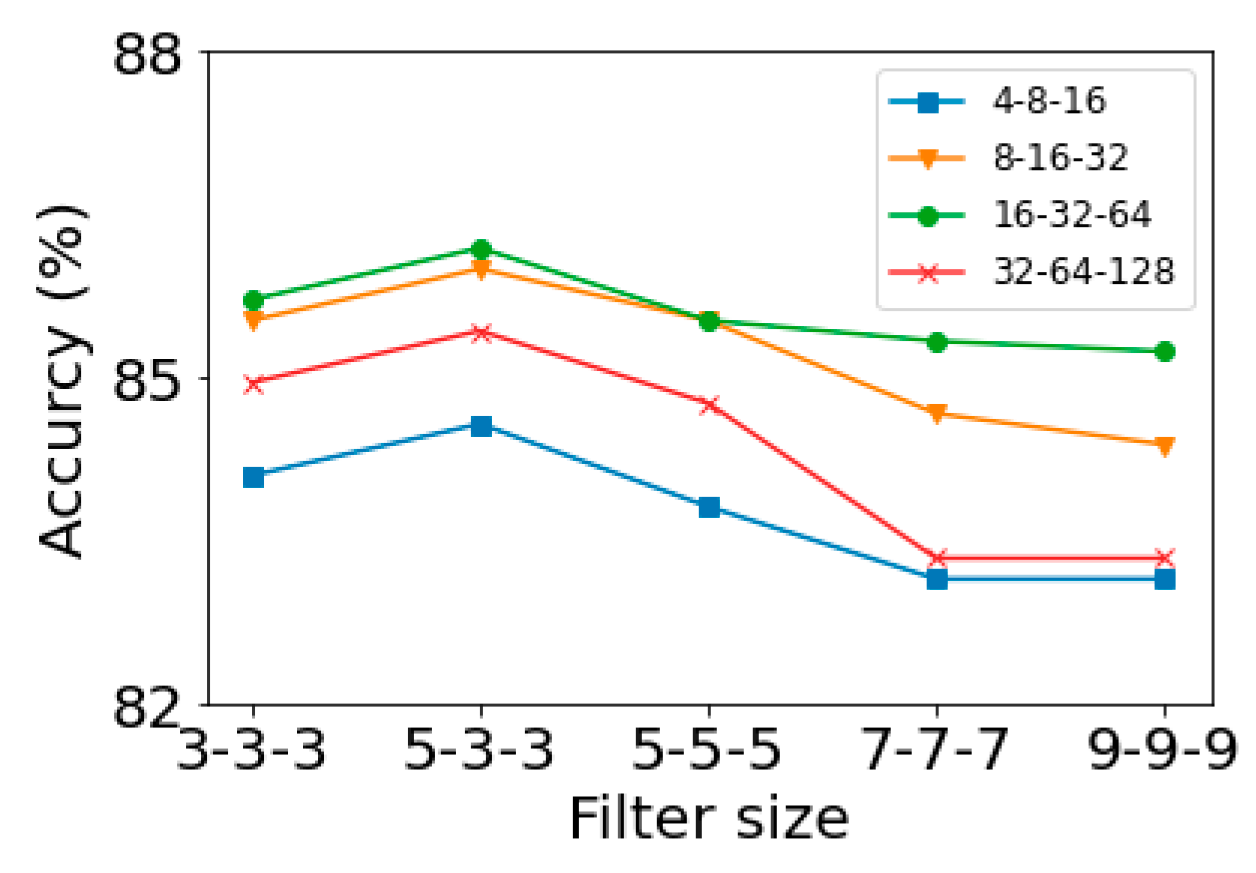
Tuning hyperparameters for CNN is difficult as it has many parameters to setup and requires long training time. For 1D CNN, we first focused on the size of filters and the number of filters. By fixing the training parameters, the grid search method was used to determine the filter size and the number of filters. Figure 9 illustrates the results obtained from various combinations of the above two parameters. Several observations can be made based on Figure 9. First, we can see that the classification accuracy decreased as the filter size increased. Second, it can be seen that using a larger filter size in the first convolution layer can improve the classification accuracy. Finally, there must be sufficient number of filters in order to have a good classification accuracy.

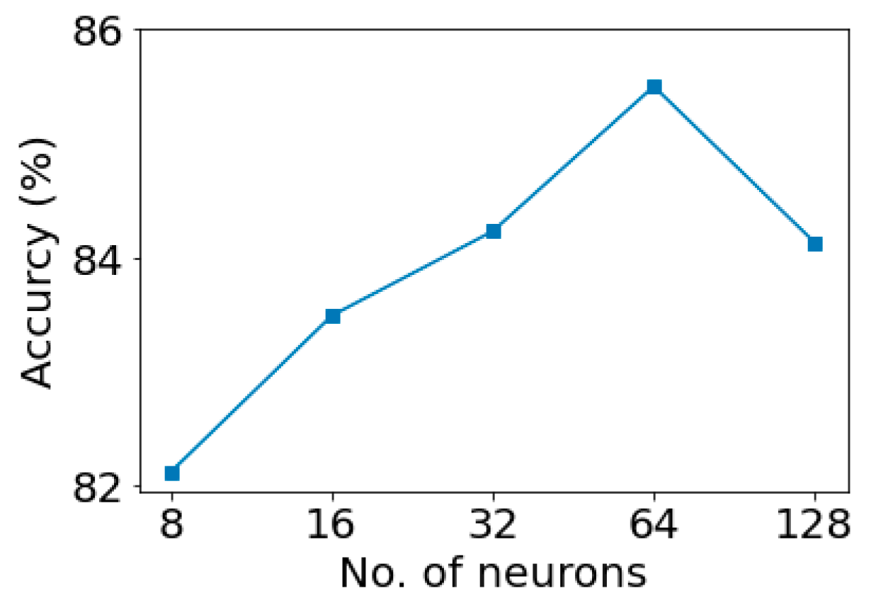
According to the results shown in Figure 10, changing the number of neurons (between 8 and 128) in the fully connected layer can improve the performance of our proposed CNN network. Based on this, the number of neurons was set to 64.

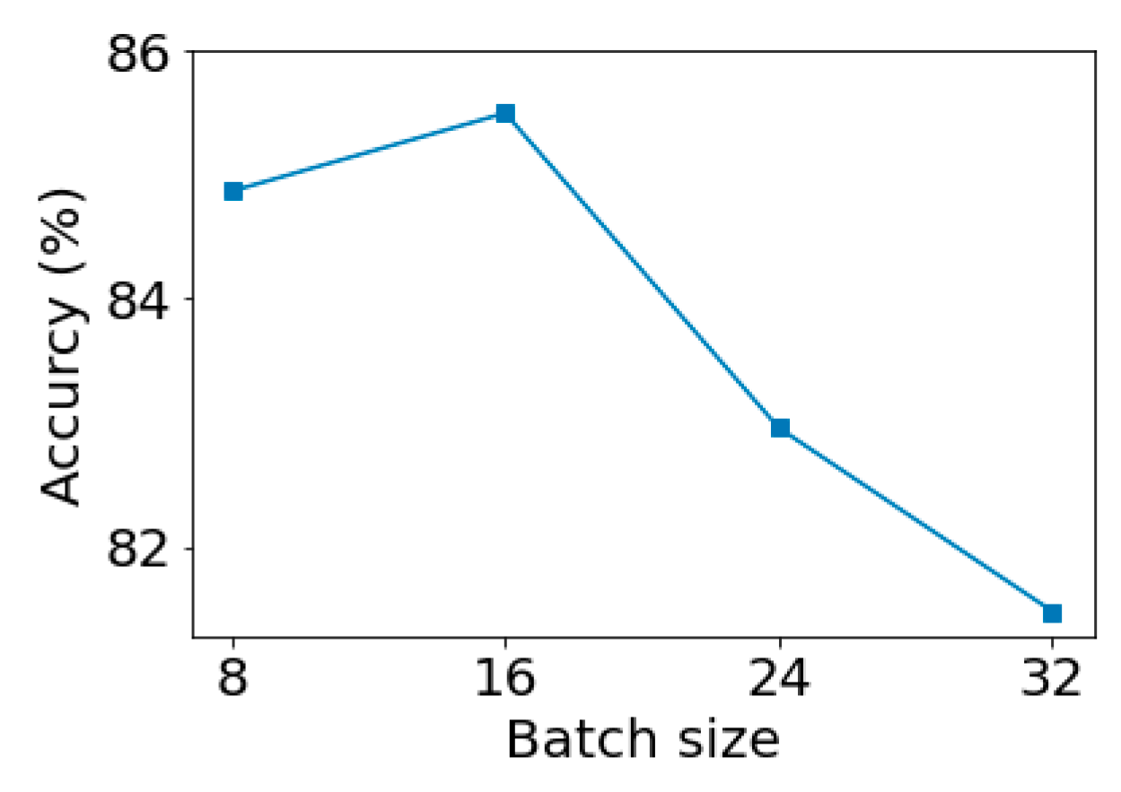
Next, we studied the effect of batch size under the condition that filter size and filter number were fixed. Figure 11 shows that the batch size influenced the accuracy of the trained model. We can see from Figure 11 that using batch size of 16 can achieve the best classification result.

With the above optimization procedure, the optimal architecture was a 1D CNN model with 3 Conv Blocks. The filter number of the convolutional layer started with 32. The filter number was increased by multiplication of 2. The filter sizes in all layers were set to 5, 3 and 3. Each convolutional layer was followed by a ReLU activation layer and a max pooling layer with the size of 2. The padding type was set to “same” to ensure that the filter could be applied to all the elements of the input. In the 1D CNN, the dropout layer was added in the second block and the third block to avoid overfitting. The dropout layer will randomly choose a ratio of neurons and update only the weights of the remaining neurons during training. The dropout ratios for the second and the third Conv Blocks were 0.2 and 0.3, respectively. After the last pooling layer, there was one fully connected layer with 64 neurons on which a dropout was applied with a ratio of 0.3. The full architecture of the 1D CNN network is summarized in

Table 2. The 1D CNN architecture.

Layer	Type	Filter Size	#Filters	Stride	Padding
1	Convolution/ReLU	$1\times 5$	16	1	same
2	Max pooling	$1\times 2$	1	2	-
3	Convolution/ReLU	$1\times 3$	32	1	same
4	Max pooling	$1\times 2$	1	2	-
5	Dropout (20%)	-	-	-	-
6	Convolution/ReLU	$1\times 3$	64	1	same
7	Max pooling	$1\times 2$	1	2	-
8	Dropout (30%)	-	-	-	-
9	Fully connected (64)	-	-	-	-
10	Dropout (30%)	-	-	-	-
11	Softmax (7)	-	-	-	-

.

The Adam optimization algorithm (learning rate 0.001) and categorical cross-entropy loss function were used to train the 1D CNN with a batch size of 16. It was trained up to 100 epochs. To avoid overfitting, early stopping criteria were implemented. This method involves stopping the training if the monitored metric has stopped improving within the five previous epochs.

The major challenge in CCPR is that many variants may encounter in real-time and on-line applications. It is useful to increase the diversity in training dataset to improve the classification accuracy. We created an augmented training dataset using the methods described above. The augmented dataset contained a total of 3150 patterns, evenly distributed among the seven pattern types.

Table 3. Number of samples of each pattern before and after data augmentation.

Pattern	Collected Data	Raw Training Data	Raw Test Data	Backward Windowing	Inbreeding	Scaling	Addition	Translation	Noise	Total Training Data
NOR	45	30	15	120	0	0	0	0	300	450
SYS	45	30	15	92	0	28	0	0	300	450
CYC	45	30	15	52	30	38	0	0	300	450
UT	45	30	15	10	15	82	0	13	300	450
DT	45	30	15	7	20	78	0	15	300	450
US	45	30	15	33	0	0	58	29	300	450
DS	45	30	15	53	0	0	45	22	300	450
Total	315	210	105							3150

summarizes the number of samples for each pattern before and after using data augmentation.

Table 4. Comparative results of data augmentation experiments.

Algorithm	Accuracy (%) without Augmentation	Accuracy (%) with Augmentation
RF	65.43 (0.78)	83.62 (1.33)
TSF	60.29 (1.27)	73.24 (0.95)
SVC	67.62	88.57
1D CNN	85.81 (0.83)	99.05 (1.06)

Numbers in parentheses denote standard deviations.

compares the experimentation results between with or without data augmentation. Using the original training dataset, CNN achieved the highest overall classification accuracy (85.81%) followed by SVC with 67.62%, TSF with 60.29% and RF with 65.43%. On the basis of the results shown in Table 4, it can be observed that augmentation operation improved performance regardless of the model. This can be explained by the fact that augmentation increases the diversity of the training dataset and thus the robustness of the classification model. After data augmentation, CNN had the highest classification accuracy, at 99.05%, while SVC, TSF and RF had 88.57%, 73.24%, and 83.62%, respectively. The experimental results suggest that the data augmentation techniques can enhance the learning capability of the 1D CNN thus improving the classification performance.

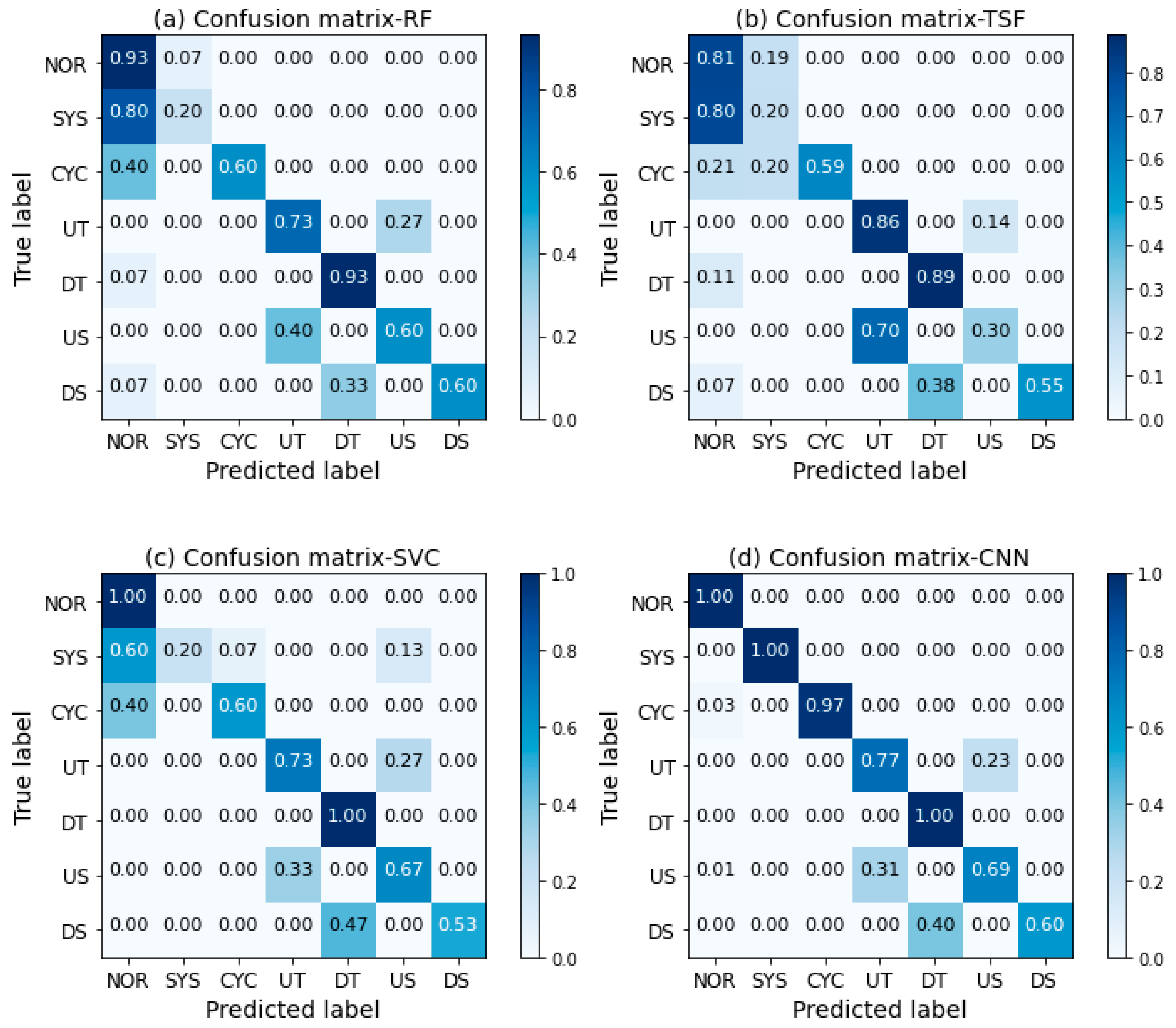
From the above results, we can see that the proposed CNN method consistently performs better than others in both settings of with/without the data augmentation strategy in terms of classification accuracy. To further examine the performance of the classification models, we check the confusion matrices shown in Figure 12 (average of 10 runs). For 1D CNN, the entries on the main diagonal are much higher than off-diagonal elements indicating a good classification model. The worse accuracies for SVC, TSF, and RF classifiers may be due to the unseen variants of non-random patterns. For RF and SVC, the systematic and cyclic pattern were the most difficult pattern types to classify. As we pointed out earlier, these classifiers treat each observation as an individual feature. Therefore, they are sensitive to the starting location of the patterns. As depicted in Figure 12, the most misclassified patterns by the feature-based TSF classifier were normal pattern, systematic and cyclic patterns. This may be explained by the fact that the features used in TSF cannot provide discriminative information among these patterns. In other words, these patterns may have similar features. This can be justified in the following experiments.

For an in-depth analysis of the deficiencies of the traditional classifiers, we studied the natures of the misclassified samples. Figure 13 illustrates some examples of misclassification by traditional classifiers. For systematic patterns, the location of the first point may affect the classification result (Figure 13a). In addition, the misclassification may be due to pattern discontinuity (Figure 13b,c). For this pattern type, discontinuity refers to the discontinued alternating up and down. The misclassification of cyclic patterns may be attributable to the translation shift or pattern discontinuity (Figure 13d–f). Here, the pattern discontinuity means the corrupted sequence of peak and valley. In practice, this may be caused by operating irregularity. Ongoing implementation of the CCPR might result in the translation shift of a pattern shown in an analysis window. The change location of trends and shifts in the analysis window might affect the classification accuracy to a great extent. If the change locations of trends were not considered in the training set, they might be misclassified as other patterns. Figure 13g,h shows the examples of misclassifying trends as shifts. Due to the same reason, the shifts may be misclassified as other pattern type (Figure 13i).

Figure 14 displays the confusion matrix for each classification model using augmented training dataset. All models gained a significant improvement in accuracy, except for TSF model. This may imply that the features adopted in TSF are not useful for patterns with observations fluctuating around the mean level. Based on the results shown in Figure 14, it can be noted that 1D CNN had much higher accuracy than RF and SVC for systematic and cyclic patterns. It appears that 1D CNN possesses the translation invariance property.

• Experiment 2: Dataset from Yu [54]

The dataset was taken from the work of Yu [54], which applied a Gaussian mixture model (GMM) for control chart pattern recognition. The author has demonstrated the adaptive capability of the proposed model with respect to novel or unknown patterns. There were six pattern types in Yu’s study, including a normal pattern and five non-random patterns (CYC, UT, DT, US, and DS). Systematic and mixture patterns were used as novel patterns. For all non-random patterns, the change points were randomly chosen around half of the time window (64). This setting makes it unique from other studies. Its uniqueness lies in the fact that there were many in-control observations preceded the non-random pattern. In the training set, there were 200 samples for each pattern, and in the test data set, there were 100 samples for each pattern. Statistical and wavelet features were generated as the inputs of GMM to implement control chart pattern recognition.

In this experiment, the proposed architecture contained three convolutional blocks, one fully connected layer, and a softmax as the output layer. The first Conv Block comprised 32 filters with a filter size of 5, and the second Conv Block comprised 128 filters with a filter size of 3. The last Conv Block had 256 filters with a filter size of 3. Each convolutional layer was followed by a ReLU activation layer and a max pooling layer with the size of 2. The dropout ratios for the second and the third Conv Blocks were set to 0.3. After the last pooling layer, there was one fully connected layer with 32 neurons on which a dropout was applied with a ratio of 0.1. The training procedure was exactly the same as that described in experiment 1.

Using the procedure described in experiment 1, the number of trees for RF was 900. TSF was trained with 600 trees with minimum interval set to 5. SVC used RBF kernel function. After a grid search study, the parameters $C$ and $\gamma$ were set to 8.0 and $2^{-6}$, respectively.

Following the evaluation of 10 different runs used by the original paper, the classification results of each classifier are summarized in

Table 5. Performance statistics of experiment 2.

Statistics/Algorithm	RF	TSF	SVC	1D CNN
Maximum	98.33	98.67	-	99.50
Minimum	97.83	98.33	-	98.83
Average (%)	98.10	98.52	98.17	99.07
StdDev	0.18	0.12	-	0.24

. We report the mean, standard deviation, minimum and maximum classification accuracy. The classification model developed by Yu [54] yielded an accuracy rate of 94.28%. The proposed 1D CNN obtained an accuracy of 99.07%. Results has also shown that CNN had the best results compared with other competitors. It is important to note that TSF outperformed RF and SVC. This is due to the fact that systematic patterns were not considered in this experiment. As explained in experiment 1, the features of TSF are not helpful for distinguishing normal and systematic patterns.

Figure 15 illustrates the confusion matrices of the worst case for Yu’s work and our 1D CNN. Matrix(a) was taken from [54] with a rearrangement of presentation order. Both methods provided perfect classification for normal and cyclic patterns. However, the method of Yu [54] had difficulty in distinguishing trends from shifts while 1D CNN performed quite well for these two pattern types.

For further assessment of the CNN model, a visualization of the learned features from different layers of 1D CNN is provided to illustrate the separation in the feature space. This was accomplished by using the t-stochastic neighbor embedded (t-SNE) clustering algorithm [55] on different layer features of the 1D CNN. The learning results for some selected layers of the CNN are visualized sequentially in Figure 16. It is clear that data points of the six pattern types in the input layer were mixed together. After the first convolution layer, data points of six classes gradually split. In the FC layers, samples of six classes were complete separate. The results show a layer by layer improvement in classification performance by transforming the low-level input data into high-level features.

• Experiment 3: Publicly Available Dataset

In this experiment, we evaluated and compared the performances of our proposed CNN using the publicly available dataset (SyntheticControl) from UCR time series classification archive [56]. This dataset was originally constructed by Alcock and Manolopoulos [57]. The window size was set to 60. The dataset included data from six control chart patterns, including NOR, CYC, UT, DT, US, and DS. There were 600 samples in total with 100 samples for each pattern type. In UCR, the original dataset has been split into training and test sets of the same size. The explicit split of training/test set of this dataset allows a direct comparison of different classification methods.

The distinguishing feature of this dataset is that the random noises follow a uniform distribution instead of normal distribution. The time series has been scaled such that each individual series has zero mean and unit variance. With this scaling, the magnitude of the individual series will be lost. In other words, the classifier receives inputs of similar magnitude.

Considering that the complexity of this dataset is not high, the selected architecture was a 1D CNN model with 2 Conv Blocks. The first Conv Block comprised 32 filters with a filter size of 5, and the second Conv Block had 128 filters with a filter size of 3. Drop out was applied to the second convolution layer with ratio 0.3. Each convolutional layer was followed by a ReLU activation layer and a max pooling layer with the size of 2. The fully connected layer included 64 neurons, followed by a dropout layer with a ratio of 0.3. The learning batch size was set to 16. The training procedure followed that described in experiment 1.

By means of the procedure described in experiment 1, the number of trees for RF and TSF were 900 and 1500, respectively. The minimum interval length of TSF was set to 3. SVC used RBF as kernel function. Using a grid search, the parameters $C$ and $\gamma$ were set to 8.0 and $2^{-5}$, respectively.

The results of different classifiers on UCR dataset are shown in

Table 6. Performance of different classification methods on publicly available dataset.

Statistics/Algorithm	RF	TSF	SVC	1D CNN
Maximum	97.00	99.33	-	100.00
Minimum	95.33	99.00	-	99.33
Average	96.17	99.20	98.33	99.60
StdDev	0.57	0.17	-	0.21

. On the basis of the results shown in Table 6, it can be seen that our 1D CNN had the highest accuracy, followed by TSF, SVC and then RF.

The results of our proposed model also outperformed most published results on this dataset. The Supervised Time Series Forest (STSF) algorithm developed by Cabello et al. [58] obtained an accuracy of 99.03% (average of ten runs). STSF is a time series forest for classification and feature extraction based on some discriminatory intervals. The time series classification with a bag of features proposed by Baydogan et al. [59] achieved accuracy of 99.1% (average of ten runs). Chen and Shi [60] reported an accuracy of 99.7% using a multi-scale convolutional neural network (MCNN). They used recurrence plot to transform original input data into 2D images. The best classification accuracy for this dataset was 100% accuracy using a collective of transformation-based ensembles (COTE) developed by Bagnall et al. [61]. However, the high computational demand of COTE is a problem in practical application.

• Experiment 4: A Simulated Dataset

The purpose of experiment 4 is to investigate the performance of CNN under a complicated situation involving high intra-class variability and high inter-class similarity. The formulas described in earlier section were used to generate the training and test datasets. The window size was set to 32. There were eight pattern types in this experiment, including a normal pattern (NOR) and seven non-random patterns (SYS, CYC, UT, DT, US, DS, and MIX). For all non-random patterns, the change point was determined by the quantity $t_0$, which is randomly chosen from a predefined range. In the training set, there were 1000 samples for each pattern, and in the test data set, there were also 1000 samples for each pattern. The pattern parameters are summarized in

Table 7. Parameters for simulating control chart patterns.

Pattern	Pattern Parameters
Systematic	$t_0\in \left\{1~17\right\}$$,{\Delta }_1\in \left\{1.5,2,2.5,3\right\}$
Cycle	$\mathsf{\Omega }\in \left\{8,16\right\}, t_0\in \left\{1~17\right\}$$,\mathsf{\kappa }\in \left\{1.5,2,2.5,3\right\}$
Trend	$t_0\in \left\{1~9\right\}$, $\theta \in \left\{0.05,0.075,0.1,0.125,0.15\right\}$
Shift	$t_0\in \left\{1~25\right\}$$,{\Delta }_2\in \left\{1.5,2,2.5,3\right\}$
Mixture	$t_0=1$$,{\mathsf{\Delta }}_3^{+}\in \left\{1.5,2,2.5,3\right\}$$,{\mathsf{\Delta }}_3^{-}\in \left\{-1.5,-2,-2.5,-3\right\}$

. The parameters are expressed in terms of standard deviation units.

The unique features of the dataset created in this experiment include the following points. For systematic pattern, it can be preceded by a certain number of in-control data. The first point of the pattern may be located above or below the mean in the analysis window. For cyclic pattern, we considered phase shift of pattern. The cycle can also be preceded by a certain number of in-control data. The trends can be preceded by a certain number of in-control data. For shift patterns, we considered the partial-shifted or full-shifted patterns in the window. For mixture, the first point may locate above or below the mean. The shifting of distributions is controlled by a random number.

Following the procedure described in experiment 1, the number of trees for RF and TSF were set to 1200 and 900, respectively. The minimum interval length of TSF was set to 5. For SVC, the parameters $C$ and $\gamma$ were set to 1.0 and $2^{-4}$, respectively.

The optimal 1D CNN architecture included three Conv Blocks. The first convolution layer was composed of 32 filters with a filter size of 5, and the second convolution layer comprised 128 filters with a filter size of 3. The last convolution layer had 256 filters with a filter size of 3. Each convolutional layer was followed by a ReLU activation layer and a max pooling layer with the size of 2. The dropout ratios for the second and the third Conv Blocks were set to 0.3. After the last pooling layer, there was one fully connected layer with 128 neurons. We applied a dropout layer after the fully connected layer and used a ratio of 0.3. The batch size was set to 512.

For the nondeterministic classifiers (e.g., RF, TSF, and CNN), we computed the average classification accuracy over 10 runs. A quantitative comparison of accuracy for individual classifier is summarized in

Table 8. Performance statistics of experiment 4.

Statistics\Algorithm	RF	TSF	SVC	1D CNN
Average	91.91	93.23	94.16	95.56
StdDev	0.13	0.09	-	0.04

. The results show that the proposed 1D CNN model outperformed all other methods in terms of mean accuracy and standard deviation.

• Experiment 5: Effects of Sample Size

In this experiment, we investigated the effect of training sample size on the classification performance. The aforementioned four datasets were considered. Using resampling from the original training dataset, we computed the classification performance on the original test dataset. For each training sample size, we performed ten runs using different random seeds. We reported the results under different numbers of training samples per class. The results are summarized in Figure 17. The x-axis shows the number of samples used per class, ranging from 1 to the full training dataset. It can be seen that the accuracy rate increased as the sample size increased. However, after the training data reached sufficient size, additional training data had a little effect on performance. We can see that the sample number required for an acceptable performance level depends on complexity of the problem to be solved. For data with extra high intra-class diversity (e.g., dataset for experiment 4), a minimum of 200 samples per class is required. For moderate intra-class diversity (e.g., datasets for experiments 1 and 2), using 20 samples per class can achieve a satisfactory performance level. For dataset with high inter-class diversity and low intra-class diversity (e.g., experiment 3), using 10 samples per class could yield an adequate performance level.

• Experiment 6: Transfer Learning

Machine learning requires a large amount of training data to establish an effective classification model. In CCPR, training data are expensive or difficult to collect. If the underlying distribution of the non-random patterns is known, one can resort to the simulation approach to create the required amount of data. However, in real-world applications we may encounter the situations where data distribution type is not known or the pattern cannot be expressed as a simple equation. In this experiment we studied the application of transfer learning to the CCPR tasks. We applied the pre-trained model developed for normally distributed data (source data) to other unknown distribution data (target data) to demonstrate the benefits of transfer learning. Labels for both the source and target data were assumed available.

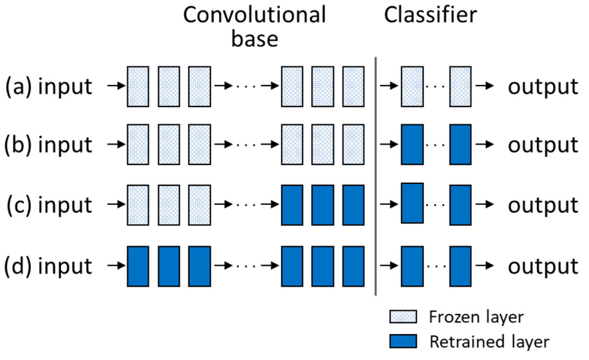
In this experiment, we studied the strategy that may yield the best results on control chart pattern recognition. In the first approach, the pre-trained model was used as a classifier, in other words, the whole model was frozen. In the second approach, we used the pre-trained model as a feature extractor for the new task. We froze the convolutional base and trained the fully connected layer. In the third approach, the whole pre-trained model was allowed to be retrained. The weights of the pre-trained model were used as the starting point of the new task.

The model described in experiment 4 was used as the basis for transfer learning in CCPR applications. We selected the gamma distribution to represent the case of skewed distributions and the uniform distribution to represent symmetric distributions with heavier tails than the normal. The gamma distribution with shape parameter $a$ and scale parameter $b$ will be denoted here by $\mathrm{G}\left(a,b\right)$. We assume $b=1$ without any loss of generality. Notice that as shape parameter $a$ increases, the gamma distribution becomes more like a normal distribution [1].

The classification performances of the CNN for various non-normal distributions are summarized in

Table 9. Classification accuracies (%) of different transfer learning strategies.

Strategy/Distribution	Uniform	G(0.5,1)	G(1,1)	G(2,1)	G(3,1)	G(4,1)	G(100,1)
Classifier	89.78 (0.24)	94.50 (0.15)	94.95 (0.11)	95.16 (0.08)	95.23 (0.07)	95.26 (0.05)	95.31 (0.09)
Feature extractor	94.42 (0.11)	98.65 (0.06)	98.08 (0.04)	97.41 (0.06)	96.81 (0.07)	96.65 (0.06)	95.62 (0.06)
Weight initialization	97.69 (0.05)	99.80 (0.03)	99.60 (0.03)	98.90 (0.04)	98.25 (0.05)	97.71 (0.05)	95.75 (0.03)
Train from scratch	97.16 (0.21)	99.62 (0.08)	99.35 (0.11)	98.72 (0.12)	97.94 (0.13)	97.51 (0.11)	95.23 (0.14)

. The number in parentheses denotes the standard deviation over ten runs. The classification performances of the models trained from scratch are also provided for ease of reference. From the results of model trained from scratch, we can observe that the highly skewed distributions lead to a large increase in classification rate. If the pre-trained model was used as a classifier, the classification accuracy for each non-normal distribution was much lower than that of the model trained from scratch. The largest discrepancy occurred when the target data followed a uniform distribution. When the pre-trained model was applied directly to $\mathrm{G}\left(100,1\right)$, it performed similar to the model trained from scratch. This is understandable because the distributional characteristics of $\mathrm{G}\left(100,1\right)$are similar to those used in the pre-trained model (i.e., normally distributed data). For the other two transfer learning approaches, we can see that the pre-trained model still performed well in the cases of non-normal distributions. It is obvious that weight initialization approach performed consistently better than just using the extracted features. This approach even performed better than the model trained from scratch (starting from random initialized parameters).

In order to further examine the benefit of using transfer learning where labelled training data on the target dataset are scarce, we carried out additional experiments with reduced amounts of training data. For all target datasets, we randomly reduced the training dataset to 5, 20, 40, and 60% of its original size. The classification performances were computed on the original test dataset.

Table 10. Comparison of models for different ratios of training dataset.

Training Target Data Proportion (%)	Uniform	G(0.5,1)	G(1,1)	G(2,1)	G(3,1)	G(4,1)	G(100,1)
5	92.04 (0.48)	97.87 (0.14)	97.52 (0.11)	96.67 (0.18)	95.41 (0.10)	95.31 (0.14)	95.13 (0.10)
20	95.18 (0.16)	99.44 (0.04)	98.93 (0.04)	98.24 (0.05)	97.12 (0.06)	96.78 (0.10)	95.21 (0.10)
40	96.61 (0.07)	99.54 (0.04)	99.29 (0.05)	98.62 (0.05)	97.74 (0.09)	97.32 (0.09)	95.44 (0.09)
60	97.15 (0.05)	99.69 (0.03)	99.49 (0.04)	98.70 (0.03)	98.06 (0.05)	97.51 (0.06)	95.74 (0.05)

displays the classification accuracy (%) for different training sample sizes. The number in parentheses denotes the standard deviation over ten runs. After close examination of the results, some interesting findings can be highlighted. First, the results indicate that the performance was affected by the variations in quantity of the training data on the target domain. A noticeable decrease in the classification accuracy occurred when the proportion of the training data was lower than 5% of the original size. When the training dataset reached 60% of its original size, the classification model nearly had the same performance as the model trained with full dataset (results of weight initialization in Table 9). The overall results suggest that transfer learning is a promising approach for CCPR when the data are scarce.

5. Conclusions

In this study, we proposed a method based on 1D CNNs to classify control chart patterns. The proposed end-to-end 1D CNN can learn the relevant features directly from the raw data without the need of feature engineering. We provided a detailed description regarding the design of CNN architecture and the determination of hyperparameters. We proposed a new pattern generator to increase pattern diversity. The results show that dataset with high diversity is useful in creating a robust classification model.

The proposed method has been evaluated on various datasets, including real-world data and simulated data. We conducted a series of experiments in response to the issues raised by previous researchers, such as the impact of the size of training set and the choice among different classification models. Through the experimental analysis, we found that the proposed 1D CNN outperformed other classifiers. We also proposed several methods suitable for augmenting the control chart dataset. The results indicate that applying data augmentation can further improve the classification accuracy for different variants of non-random patterns.

This study also investigated the usefulness of transfer learning techniques to control chart pattern recognition task. The pre-trained model using normally distributed data was used as a starting point and fine-tuned on the unknown non-normal data. Different transfer learning approaches were investigated. Our experimental results indicate that fine-tuning approach performed consistently better than just using the extracted features. The results also show that the fine-tuning approach even outmatched the model trained from scratch. The overall results may suggest that transfer learning is a promising approach when the data are scarce.

In summary, the model and methods proposed in this study can effectively improve the classification accuracy of control chart patterns. Based on the results of this study, we may conclude that 1D convolutional neural networks are a promising alternative to feature-based classifiers for control chart pattern classification. The results and findings of this study are crucial for the further realization of smart statistical process control.

An apparent limitation of the proposed method is the reliance on a training set with well-separated pattern type and it would take a lot of time. One solution is to apply the unsupervised clustering algorithm to separate pattern data corresponding to out-of-control situations. This is an area for future research to explore.

The magnitudes of non-random patterns considered in this study were similar to those used in previous research. It is realized that this setting may result in many observations falling outside of the control limits. In some applications, we may want to apply the CCPR even when the observations fall within the control limits. In such a case, we have to consider small magnitude of changes in the training set. By doing so, non-random patterns may interfere with each other causing a decrease in classification accuracy. Future research should investigate the effect of including patterns with small magnitudes in the training dataset. The present study considered the CCPR on basic non-random patterns. Further research might investigate the application of 1D CNN to processes with concurrent patterns. Applying 1D CNN to CCPR of multivariate SPC may also be a topic worthy of further exploration.

References

1. Montgomery, D.C. Introduction to Statistical Quality Control, 8th ed.; John Wiley & Sons: New York, NY, USA, 2020. [Google Scholar]
2. Jang, K.Y.; Yang, K.; Kang, C. Application of artificial neural network to identify non-random variation patterns on the run chart in automotive assembly process. Int. J. Prod. Res. 2003, 41, 1239–1254. [Google Scholar] [CrossRef]
3. Chiu, S.H.; Lu, C.P. On-line unusual tension recognition system on twister using smooth support vector machine classifier. Int. J. Adv. Manuf. Syst. 2006, 30, 92–97. [Google Scholar] [CrossRef]
4. Western Electric. Statistical Quality Control Handbook; Western Electric Company: Indianapolis, IN, USA, 1956. [Google Scholar]
5. Nelson, L.S. The Shewhart control chart tests for special causes. J. Qual. Technol. 1984, 16, 237–239. [Google Scholar] [CrossRef]
6. Nelson, L.S. Interpreting Shewhart X control chart. J. Qual. Technol. 1985, 17, 114–116. [Google Scholar] [CrossRef]
7. Cheng, C.S. A neural network approach for the analysis of control chart patterns. Int. J. Prod. Res. 1997, 35, 667–697. [Google Scholar] [CrossRef]
8. Zan, T.; Liu, Z.; Wang, H.; Wang, M.; Gao, X. Control chart pattern recognition using the convolutional neural network. J. Intell. Manuf. 2020, 31, 703–716. [Google Scholar] [CrossRef]
9. Reis, M.S.; Gins, G. Industrial process monitoring in the big data/industry 4.0 era: From detection, to diagnosis, to prognosis. Processes 2017, 5, 35. [Google Scholar] [CrossRef] [Green Version]
10. Hachicha, W.; Ghorbel, A. A survey of control chart pattern recognition literature (1991–2010) based on a new conceptual classification scheme. Comput. Ind. Eng. 2012, 63, 204–222. [Google Scholar] [CrossRef]
11. Evans, J.R.; Lindsay, W.M. A framework for expert system development in statistical quality control. Comput. Ind. Eng. 1988, 14, 335–343. [Google Scholar] [CrossRef]
12. Cheng, C.S.; Hubele, N.F. Design of a knowledge-based expert system for statistical process control. Comput. Ind. Eng. 1992, 22, 501–517. [Google Scholar] [CrossRef]
13. Pham, D.T.; Wani, M.A. Feature-based control chart pattern recognition. Int. J. Prod. Res. 1997, 35, 1875–1890. [Google Scholar] [CrossRef]
14. Bag, M.; Gauri, S.K.; Chakraborty, S. An expert system for control chart pattern recognition. Int. J. Adv. Manuf. Syst. 2012, 62, 291–301. [Google Scholar] [CrossRef]
15. Pham, D.T.; Oztemel, E. Control chart pattern recognition using neural networks. J. Syst. Eng. 1992, 2, 256–262. [Google Scholar]
16. Guh, R.S.; Tannock, J.D.T. Recognition of control chart concurrent patterns using a neural network approach. Int. J. Prod. Res. 1999, 37, 1743–1765. [Google Scholar] [CrossRef]
17. Ranaee, V.; Ebrahimzadeh, A.; Ghaderi, R. Application of the PSO-SVM model for recognition of control chart patterns. ISA Trans. 2010, 49, 577–586. [Google Scholar] [CrossRef] [PubMed]
18. Zhang, M.; Yuan, Y.; Wang, R.; Cheng, W. Recognition of mixture control chart patterns based on fusion feature reduction and fireworks algorithm-optimized MSVM. Pattern Anal. Appl. 2020, 23, 15–26. [Google Scholar] [CrossRef]
19. Chen, Z.; Lu, S.; Lam, S. A hybrid system for SPC concurrent pattern recognition. Adv. Eng. Inform. 2007, 21, 303–310. [Google Scholar] [CrossRef]
20. Yang, W.A.; Zhou, W.; Liao, W.; Gou, Y. Identification and quantification of concurrent control chart patterns using extreme-point symmetric mode decomposition and extreme learning machines. Neurocomputing. 2015, 147, 260–270. [Google Scholar] [CrossRef]
21. Gauri, S.K.; Chakraborty, S. Recognition of control chart patterns using improved selection of features. Comput. Ind. Eng. 2009, 56, 1577–1588. [Google Scholar] [CrossRef]
22. Ranaee, V.; Ebrahimzadeh, A. Control chart pattern recognition using neural networks and efficient features: A comparative study. Pattern Anal. Appl. 2013, 16, 321–332. [Google Scholar] [CrossRef]
23. Addeh, A.; Khormali, A.; Golilarz, N.A. Control chart pattern recognition using RBF neural network with new training algorithm and practical features. ISA Trans. 2018, 79, 202–216. [Google Scholar] [CrossRef]
24. Shorten, C.; Khoshgoftaar, T.M. A survey on image data augmentation for deep learning. J. Big Data 2019, 6, 60. [Google Scholar] [CrossRef]
25. Du, W.; Wang, S.; Gong, X.; Wang, H.; Yao, X.; Pecht, M. Translation invariance-based deep learning for rotating machinery diagnosis. Hindawi Shock. Vib. 2020, 2020, 1635621. [Google Scholar] [CrossRef]
26. Woodall, W.H.; Montgomery, D.C. Some current directions in the theory and application of statistical process monitoring. J. Qual. Technol. 2014, 46, 78–94. [Google Scholar] [CrossRef]
27. Weese, M.; Martinez, W.; Megahed, F.M.; Jones-Farmer, L.A. Statistical learning methods applied to process monitoring: An overview and perspective. J. Qual. Technol. 2016, 48, 4–24. [Google Scholar] [CrossRef]
28. Hong, Z.; Li, Y.; Zeng, Z. Convolutional neural network for control chart patterns recognition. In Proceedings of the CSAE 2019: 3rd International Conference on Computer Science and Application Engineering, Sanya, China, 22–24 October 2019. [Google Scholar]
29. Miao, Z.; Yang, M. Control chart pattern recognition based on convolution neural network. In Smart Innovations in Communication and Computational Sciences; Advances in Intelligent Systems and Computing (AISC) 670; Panigrahi, B., Trivedi, M., Mishra, K., Tiwari, S., Singh, P., Eds.; Springer: Singapore, 2019; pp. 97–104. [Google Scholar]
30. Xu, J.; Lv, H.; Zhung, Z.; Lu, Z.; Zou, D.; Qin, W. Control chart pattern recognition method based on improved one-dimensional convolutional neural network. IFAC PapersOnLine 2019, 52, 1537–1542. [Google Scholar] [CrossRef]
31. Yu, J.; Zheng, X.; Wang, S. A deep autoencoder feature learning method for process pattern recognition. J. Process. Control. 2019, 79, 1–15. [Google Scholar] [CrossRef]
32. Chu, H.; Zhao, K.; Cheng, Q.; Li, R.; Yang, C. Control chart patterns recognition based on optimized deep belief neural network and data information enhancement. IEEE Access 2020, 8, 203685–203699. [Google Scholar] [CrossRef]
33. Fuqua, D.; Razzaghi, T. A cost-sensitive convolution neural network learning for control chart pattern recognition. Expert Syst. Appl. 2020, 150, 113275. [Google Scholar] [CrossRef]
34. Zan, T.; Liu, Z.; Su, Z.; Wang, M.; Gao, X.; Chen, D. Statistical process control with intelligence based on the deep learning model. Appl. Sci. 2020, 10, 308. [Google Scholar] [CrossRef] [Green Version]
35. Al-Saffar, A.A.M.; Tao, H.; Talab, M.A. Review of deep convolution neural network in image classification. In Proceedings of the 2017 International Conference on Radar, Antenna, Microwave, Electronics, and Telecommunications (ICRAMET), Jakarta, Indonesia, 23–24 October 2017; Institute of Electrical and Electronics Engineers (IEEE): Piscataway, NJ, USA, 2017. [Google Scholar]
36. Aloysius, N.; Geetha, M. A review on deep convolutional neural networks. In Proceedings of the 2017 International Conference on Communication and Signal Processing (ICCSP), Chennai, India, 6–8 April 2017; Institute of Electrical and Electronics Engineers (IEEE): Piscataway, NJ, USA, 2017. [Google Scholar]
37. Ajit, A.; Acharya, K.; Samanta, A. A review of convolutional neural networks. In Proceedings of the 2020 International Conference on Emerging Trends in Information Technology and Engineering (ic-ETITE), Vellore, India, 24–25 February 2020; Institute of Electrical and Electronics Engineers (IEEE): Piscataway, NJ, USA, 2020. [Google Scholar]
38. Fawaz, H.I.; Forestier, G.; Weber, J.; Idoumghar, L.; Muller, P.A. Deep learning for time series classification: A review. Data Min. Knowl. Discov. 2019, 33, 917–963. [Google Scholar] [CrossRef] [Green Version]
39. Kiranyaz, S.; Avci, O.; Abdeljaber, O.; Ince, T.; Gabbouj, M.; Inman, D.J. 1D convolutional neural networks and applications: A survey. Mech. Syst. Signal Process. 2021, 151, 107398. [Google Scholar] [CrossRef]
40. Chollet, F. Keras. 2015. Available online: https://github.com/fchollet/keras (accessed on 13 July 2021).
41. Vapnik, V.N. The Nature of Statistical Learning Theory; Springer: New York, NY, USA, 1995. [Google Scholar]
42. Pedregosa, F.; Varoquaux, G.; Gramfort, A.; Michel, V.; Thirion, B.; Grisel, O.; Blondel, M.; Prettenhofer, P.; Weiss, R.; Dubourg, V. Scikit-learn: Machine learning in Python. J. Mach. Learn. Res. 2011, 12, 2825–2830. [Google Scholar]
43. Breiman, L. Random forests. Mach. Learn. 2001, 45, 5–32. [Google Scholar] [CrossRef] [Green Version]
44. Deng, H.; Runger, G.; Tuv, E.; Vladimir, M. A time series forest for classification and feature extraction. Inf. Sci. 2013, 239, 142–153. [Google Scholar] [CrossRef] [Green Version]
45. Pan, S.J.; Yang, Q. A survey of transfer learning. IEEE Trans. Knowl. Data. Eng. 2010, 22, 1345–1359. [Google Scholar] [CrossRef]
46. Zhuang, F.; Qi, Z.; Duan, K.; Xi, D.; Zhu, Y.; Zhu, H.; Xiong, H.; He, Q. A comprehensive survey on transfer learning. Proc. IEEE 2021, 109, 43–76. [Google Scholar] [CrossRef]
47. Guo, Y.; Shi, H.; Kumar, A.; Grauman, K.; Rosing, T.; Feris, R. SpotTune: Transfer learning through adaptive fine-tuning. In Proceedings of the 2019 IEEE Conference on Computer Vision and Pattern Recognition (CVPR), Long Beach, LA, USA, 15–21 June 2019; Institute of Electrical and Electronics Engineers (IEEE): Piscataway, NJ, USA, 2019; pp. 4805–4814. [Google Scholar]
48. Vrbančič, G.; Podgorelec, V. Transfer learning with adaptive fine-tuning. IEEE Access 2020, 8, 196197–196211. [Google Scholar] [CrossRef]
49. Rashid, K.M.; Louis, J. Times-series data augmentation and deep learning for construction equipment activity recognition. Adv. Eng. Inform. 2019, 42, 100944. [Google Scholar] [CrossRef]
50. Oh, C.; Han, S.; Jeong, J. Time-series data augmentation based on interpolation. Procedia Comput. Sci. 2020, 175, 64–71. [Google Scholar] [CrossRef]
51. Liu, B.; Zhang, Z.; Cui, R. Efficient time series augmentation methods. In Proceedings of the 2020 13th International Congress on Image and Signal Processing, BioMedical Engineering and Informatics (CISP-BMEI), Online, 17–19 October 2020; Available online: https://ieeexplore.ieee.org/document/9263602 (accessed on 22 August 2021).
52. Wen, Q.; Sun, L.; Yang, F.; Song, X.; Gao, J.; Wang, X.; Xu, H. Time series data augmentation for deep learning: A survey. arXiv 2021, arXiv:2002.12478. [Google Scholar]
53. Löning, M.; Bagnall, A.; Ganesh, S.; Kazakov, V.; Lines, J.; Király, F.J. Sktime: A unified interface for machine learning with time series. In Proceedings of the 33rd Conference on Neural Information Processing Systems (NeurIPS 2019), Vancouver, BC, Canada, 8–14 December 2019. [Google Scholar]
54. Yu, G. Gaussian mixture models-based control chart pattern recognition. Int. J. Prod. Res. 2012, 50, 6746–6762. [Google Scholar] [CrossRef]
55. Van der Maaten, L.J.P.; Hinton, G.E. Visualizing data using t-SNE. J. Mach. Learn. Res. 2008, 9, 2579–2605. [Google Scholar]
56. Dau, H.A.; Bagnall, A.; Kamgar, K.; Yeh, C.M.; Zhu, Y.; Gharghabi, S.; Ratanamahatana, C.A.; Keogh, E. The UCR time series classification archive. IEEE/CAA J. Autom. Sin. 2019, 6, 1293–1305. [Google Scholar] [CrossRef]
57. Alcock, R.J.; Manolopoulos, Y. Time-series similarity queries employing a feature-based approach. In Proceedings of the 7th Hellenic Conference on Informatics, Ioannina, Greece, 26–29 August 1999. [Google Scholar]
58. Cabello, N.; Naghizade, E.; Qi, J.; Kulik, L. Fast and accurate time series classification through supervised interval search. In Proceedings of the 2020 IEEE International Conference on Data Mining (ICDM), Sorrento, Italy, 17–20 November 2020; Institute of Electrical and Electronics Engineers (IEEE): Piscataway, NJ, USA, 2020. [Google Scholar]
59. Baydogan, M.G.; Runger, G.; Tuv, E. A bag-of-features framework to classify time series. IEEE Trans. Pattern Anal. Mach. Intell. 2013, 35, 2796–2802. [Google Scholar] [CrossRef]
60. Chen, W.; Shi, K. A deep learning framework for time series classification using relative position matrix and convolutional neural network. Neurocomputing 2019, 359, 384–394. [Google Scholar] [CrossRef]
61. Bagnall, A.; Lines, J.; Hills, J.; Bostrom, A. Time-series classification with COTE: The collective of transformation-based ensembles. IEEE Trans. Knowl. Data. Eng. 2015, 27, 2522–2535. [Google Scholar] [CrossRef]
Figure 1. Typical examples of control chart patterns.
Processes 09 01484 g001
Figure 2. Variants of non-random pattern in the course of classification. (a) Original data. (bd) Data in different classification stages before being classified as non-random.
Processes 09 01484 g002
Figure 3. A 1D convolutional neural network (CNN) structure.
Processes 09 01484 g003
Figure 4. Different usages of pre-trained model: (a) Freeze the whole model. (b) Freeze the convolutional base and train the classifier. (c) Train most of the convolutional base layers and the classifier. (d) Train the whole model.
Processes 09 01484 g004
Figure 5. Variants of non-random patterns.
Processes 09 01484 g005
Figure 6. Illustration of data augmentation.
Processes 09 01484 g006
Figure 7. The effect of the number of trees.
Processes 09 01484 g007
Figure 8. Performance of SVC by varying C and γ .
Processes 09 01484 g008
Figure 9. Performance of 1D CNN by varying the filter sizes and the number of filters.
Processes 09 01484 g009
Figure 10. Performance of 1D CNN by varying the number of hidden layer neurons.
Processes 09 01484 g010
Figure 11. Performance of 1D CNN by varying batch size.
Processes 09 01484 g011
Figure 12. Confusion matrices obtained from experiment 1. Each row represents a true class, while each column represents a predicted class.
Processes 09 01484 g012
Figure 13. Examples of misclassification by traditional classifiers. (ac) SYS was misclassified as NOR. (df) CYC was misclassified as NOR. (g) UT was misclassified as US. (h) DT was misclassified as DS. (i) DS was misclassified as DT.
Processes 09 01484 g013
Figure 14. Confusion matrices obtained from experiment 1 (with data augmentation). Each row represents a true class, while each column represents a predicted class.
Processes 09 01484 g014
Figure 15. Confusion matrices for the worst case in ten runs of experiment 2. For ease of comparison, the metrices were not normalized.
Processes 09 01484 g015
Figure 16. Visualization of the learning process for experiment 2.
Processes 09 01484 g016
Figure 17. Effects of the size of training samples on classification performance.
Processes 09 01484 g017