Proton Exchange Membrane Fuel Cell Parameter Extraction Using a Supply–Demand-Based Optimization Algorithm

Abstract

For proton exchange membrane fuel cells (PEMFCs), the parameter extraction issue is among the most widely studied problems in the field of energy storage systems, since the precise identification of such parameters plays an important role in increasing the PEMFC performance and life span. The optimization process is intended to adjust the performance of PEMFCs by appraising the optimal parameters that produce a good estimation of the current–voltage (I–V) curve. In order to build an accurate equivalent circuit model for PEMFCs, a reliable and effective parameter extraction algorithm, termed a supply–demand-based optimization (SDO) algorithm, is proposed in this paper. Nine parameters (${\xi }_1, {\xi }_2, {\xi }_3, {\xi }_4, R_c, \beta , \lambda , l, and J_{max}$) are evaluated, to minimize the sum squared deviation (SSE) between the experimental and simulated I–V curves. To validate the feasibility and effectiveness of the SDO algorithm, four sets of experimental data with diverse characteristics and two well-known PEMFC stacks (BSC500W and 500W Horizon) are employed. Comparison of the simulated and experimental results clearly demonstrates the superiority/competitiveness of the SDO algorithm over five well-established parameter extraction algorithms, i.e., the whale optimization algorithm (WOA), grey wolf optimization (GWO), Harris hawks optimization (HHO), and genetic algorithm (GA). Several evaluation criteria, including best SSE, worst SSE, mean SSE, and standard deviation, show that the SDO algorithm has merits in terms of PEMFC modeling.

1. Introduction

The exponential demand for electricity and the impact of fossil fuel use, e.g., global warming, have led to an increase in the utilization of renewable energy resources (RERs). Appropriate techniques for energy storage help to deal with the lower availability of RERs, such as wind and solar energy, and thus contribute to the de-carbonization of multiple applications, e.g., automotive, grid-connection, maritime, and residential applications [1]. Among the storage system techniques, fuel cell (FC) devices have received much attention as energy storage media [2,3]. Proton exchange membrane fuel cells (PEMFCs), which ordinarily generate electricity, through a chemical reaction between hydrogen and oxygen or another oxidizing agent, have become more ubiquitous in the recent years, owing to their inherent advantages. PEMFCs have several outstanding characteristics, such as high energy efficiency; high energy density; low overall cost; low working noise; low operating temperature; zero emissions of nitrogen oxides, sulfur oxides, and CO₂; short startup time; use of solid electrolytes; zero corrosion; and long life [4].

To simulate, optimize, control, and investigate PEMFC dynamic behavior, an accurate mathematical model of PEMFCs is essential [5,6]. Mathematical modeling is important to simulate the performance of a PEMFC at different operating conditions in real work. The PEMFC model comprises several unknown parameters, and estimating their relevant values is considered difficult, because the PEMFC model is complex and nonlinear and its parameters are rigorously dependent on the adopted operating conditions [7,8]. In such a context, many optimization algorithms have been employed to attain precise values for the PEMFC parameters. Traditional algorithms, such as gradient-based optimization [9], the Newton–Raphson method [10], the conjugate-direction method [11], and linear optimization [12], are common optimization algorithms that are used for small-scale problems, owing to their deterministic feature and computational complexity. Notwithstanding the simplicity of the linear optimization approaches, significant errors may be caused in models with nonlinear features. Gradient-based optimization approaches can become easily stuck in a local optimum, causing erroneous solutions, because they depend on convex fitness. Moreover, some traditional algorithms are very sensitive to initial conditions, and potentially converge to critical solutions that are not the global optimum. These drawbacks confine the application of traditional methods to parameter estimations for PEMFCs, which require a nonlinear model and the fitness function, which exhibits nonsmooth nonconvex characteristics [7]. Moreover, the parameters of PEMFCs must be identified under different operating conditions, leading to a large, complex search space [13,14]. Due to the nature of heuristic methods, metaheuristic algorithms are gradient-free algorithms that do not use any derivatives and do not depend on domain information or the continuity/convexity of fitness functions. The great advantages of using metaheuristic algorithms are the simplicity, ease of implementation, and robustness [15]. The broad applications of metaheuristic algorithms in solving the parameter identification problems of PEMFC models, such as the genetic algorithm (GA) [16], particle swarm optimization (PSO) [17], firefly optimization (FFO) [18], grey wolf optimization (GWO) [19], simulated annealing (SA) [20], harmony search (HS) [21], artificial bee swarm (ABS) optimization [22], flower pollination algorithm (FPA) [23], artificial bee colony (ABC) algorithm [24], big bang–big crunch (BBBC) algorithm [25], salp swarm optimizer (SSA) [26], shark smell optimizer (SSO) [27], multi-verse optimizer (MVO) [28], teaching learning-based algorithm (TLBO) [29], backtracking search algorithm (BSA) [30], differential evolution algorithm (DEA) [31], biogeography-based optimization (BBO) [32], imperialist competitive algorithm (ICA) [33], grasshopper optimization algorithm (GOA) [34], bird mating optimizer (BMO) [35], flower pollination algorithm (FPA) [23], whale optimization algorithm (WOA) [36], satin bowerbird optimizer (SBO) [37], seagull optimization algorithm (SOA) [38], shuffled frog-leaping algorithm (SFLA) [33], vortex search algorithm (VSA) [39], bat algorithm (BA) [40], owl search algorithm (OSA) [18], tree growth algorithm (TGA) [41], Harris hawks optimization (HHO) [42], atom search optimizer (ASO) [43], dragonfly algorithm (DA) [44], ant lion optimizer (ALO) [44], cuckoo search algorithm (CS) [45], artificial immune system (AIS) [46], and JAYA algorithm [47], have increased, owing to their extraordinary capabilities.

Considering the foregoing, metaheuristic algorithms are often acknowledged as more efficient and effective than classical algorithms. While a certain algorithm may perform admirably when optimizing a particular sort of problem, it may be incapable of selecting the most accurate solution within the range of possible values for another design condition. Also, the results in some studies have been obtained under different design conditions, especially the termination criterion and performance factors. Moreover, due to its stochastic nature, a metaheuristic algorithm commonly produces different solutions when it is applied to a specific problem for different runs. Therefore, the average solution, standard deviation (STD), and statistical testing, should also be applied. The average solution and STD assess the overall performance, whereas statistical testing assesses each run’s solution and confirms its statistical significance.

For the first time, this study applies a recently developed and highly efficient metaheuristic algorithm, termed supply–demand-based optimization (SDO), to the parameter identification problem for PEMFCs. The SDO replicates the consumer–producer supply–demand relationship [48]. The supply–demand mechanism, according to economic principles, has the following two states: stable and instable. The quantity and cost converge to a balancing point in the stable mode, which can be adapted to the SDO as exploitation, to carry out a local pursuit. In the instable mode, the quantity and cost diverge from the balancing point and can be used in conjunction with the SDO, as exploration, to conduct a global chase in the search region. The better exploration, exploitation, and convergence rate, together with local optima avoidance, high accuracy, and lower number of parameters, are the most important reasons for studying the practical viability and rationality of SDO in the PEMFC identification problem. The main contributions of this study are as follows: (i) SDO is applied to effectively identify the parameters of PEMFC models. To our knowledge, this is the first attempt at identifying PEMFC parameters based on SDO; (ii) The performance of the PEMFC stack is thoroughly evaluated under various experimental pressure and temperature conditions. In addition, the sensitivity of SDO is explored; and (iii) The supremacy of SDO is statistically confirmed by comparison with five state-of-the-art metaheuristic algorithms, using average convergence, STD, and statistical testing.

The rest of this paper is organized as follows: Section 2 discusses the mathematical modeling of the PEMFC stack. Section 3 details the design circumstances, limitations, and SDO optimization technique. Section 4 contains experimental results, comparisons, and the discussion. Section 5 contains the work’s conclusions.

2. PEMFC Modeling

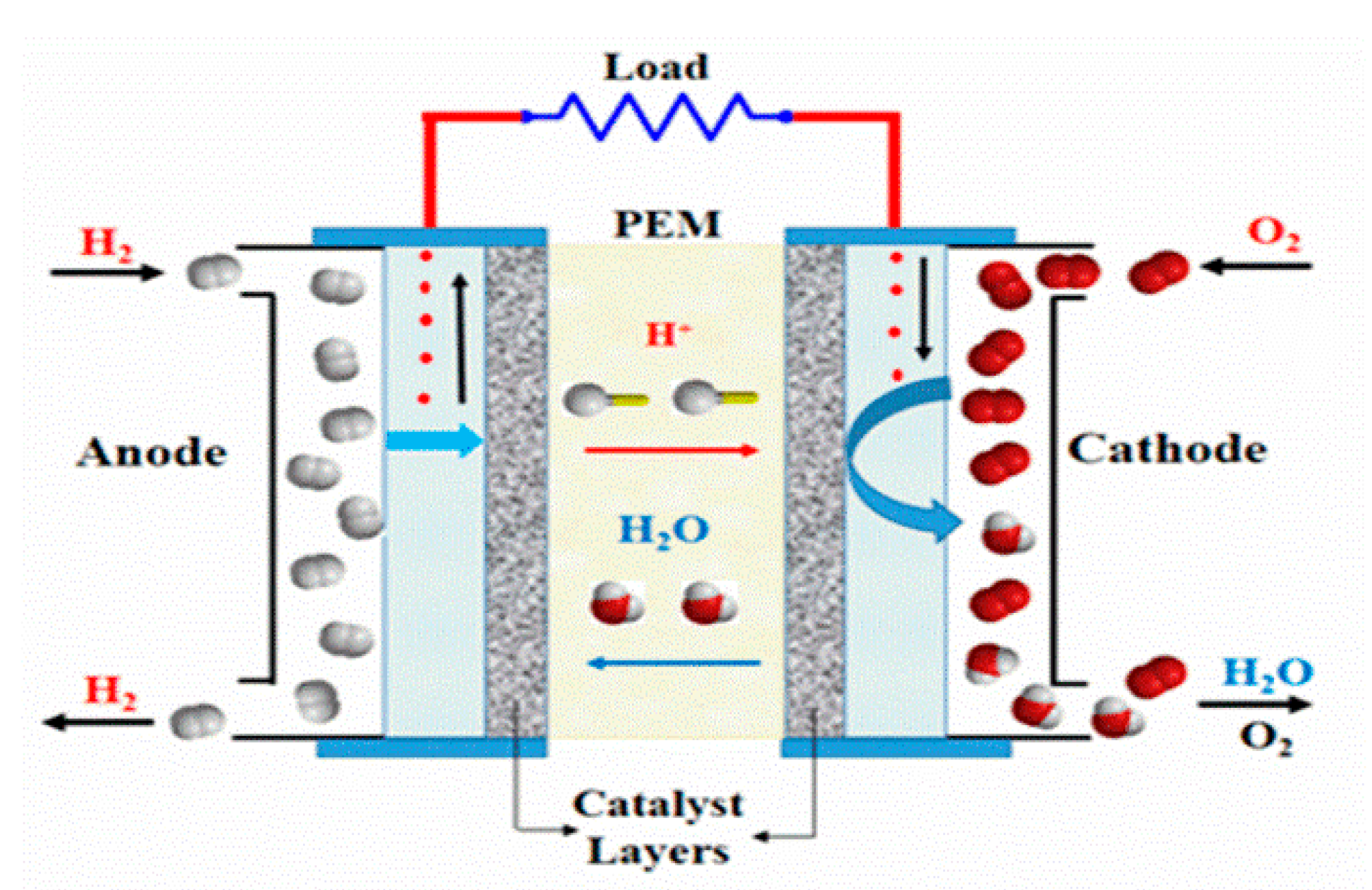
2.1. Basic Operation of PEMFC

An FC basically converts chemical energy, stored in a fuel and oxidant, directly into DC electrical energy. An FC consists of the following major structural units: catalyst layers (anode and cathode), proton exchange membrane (PEM), gas diffusion layers, and bipolar plates [49], as shown in Figure 1. In the anode layer, hydrogen reacts with a catalyst surface, producing an electron and a proton, according to Equation (1).

$$H_2 \stackrel{pt}{\to }2H^{+}+2e^{-}$$

(1)

The electron travels through a circuit to produce a current, while the proton passes through the electrolyte to the cathode side. At the cathode, oxygen reacts with the hydrogen ion and electron, producing water and heat, according to the following reaction:

$$2H^{+}+2e^{-}+1/2 O_2\stackrel{pt}{\to }{H}_{2}O+Heat$$

(2)

The overall chemical reaction occurring inside a PEMFC is calculated by the following equation:

$$2H^{+}+1/2 O_2\stackrel{pt}{\to }{H}_{2}O+Heat+Electerical energy$$

(3)

2.2. Theoretical Modeling

The terminal voltage of a PEMFC is calculated as the sum of theoretical voltage $\left(E_{Nernest}\right)$and three voltage losses, i.e., activation $\left(V_{act}\right)$, ohmic $\left(V_{ohm}\right)$, and concentration $\left(V_{con}\right)$, as shown Equation (4) [49], as follows:

$$V_{cell}=E_{Nernest}-V_{act}-V_{ohm}-V_{con}$$

(4)

The theoretical voltage can be expressed using Equation (5), which estimates the thermodynamic voltage and is expressed as [50], as follows:

$$E_{Nernst}=1.229-\frac{0.85}{{10}^3}\left(T-298.15\right)+\frac{4.31}{{10}^5}T\left(\ln \left(P_{H_2}\right)+0.5\ln \left(P_{O2}\right)\right)$$

(5)

where $T$ is the temperature of the cell (K), and$P_{H_2}$ and $P_{O2}$ are the partial gas pressures of hydrogen and oxygen, respectively. For O₂ and H₂ reactants, $P_{O2}$ is calculated using Equation (6) [51], as follows:

$$P_{O_2}=\left(R{H}_C\times P_{H_{2}O}^{sat}\right)\times \left[\frac{P_{c }\times \exp \left(\frac{-4.192\left(I/A\right)}{T^{1.334}}\right)}{R{H}_c\times P_{H_{2}O}^{sat}}-1\right]$$

(6)

where $R{H}_C$and $P_{c }$represent the relative humidity and inlet pressure (atm) at the cathode side, respectively; A is the active membrane area (cm²); and $I$ is the current of the cell (A). $P_{H2}$ can be calculated using Equation (7) [51], as follows:

$$P_{H_2}=0.5\left(R{H}_a\times P_{H_{2}O}^{sat}\right)\left[\frac{P_{a }\times \exp \left(\frac{-1.635\left(I/A\right)}{T^{1.334}}\right)}{R{H}_c\times P_{H_{2}O}^{sat}}-1\right]$$

(7)

where $R{H}_a$and $P_{a }$represent the relative humidity and inlet pressure (atm) at the anode side, respectively, and $P_{H_{2}O}^{sat}$ is the saturation pressure of water (atm), calculated from Equation (8) [52].

The activation voltage loss can be determined using Equation (9) [50].

$$lo{g}_{10}\left(P_{H_{2}O}^{sat}\right)=\frac{2.95}{{10}^2}\left(T-273.15\right)-\frac{9.18}{{10}^5}{\left(T-273.15\right)}^2+\frac{1.44}{{10}^7}{\left(T-373.15\right)}^3-2.18$$

(8)

$$V_{act}=-\left[{\xi }_1+{\xi }_2\times T+{\xi }_3\times T\times \ln \left(C_{O_2}\right)+{\xi }_4\times \ln \left(I\right)\right]$$

(9)

where ${\xi }_1, {\xi }_2, {\xi }_3, \mathrm{and} {\xi }_4$are the semi-empirical constants, and $C_{O_2}$ is the concentration of dissolved oxygen (mol cm⁻³), which can be calculated using Equation (10) [53], as follows:

$$C_{O_2}=\frac{P_{O_2}}{5.08\times {10}^6} e^{\frac{-498}{T}}$$

(10)

The ohmic voltage loss ($V_{ohm}$) can be obtained from Equation (11) [54], as follows:

$$V_{ohm}=I\left(R_m+R_C\right)$$

(11)

where $R_C$and $R_m$ are the resistance of the membrane against the transfer of protons (Ω) and the equivalent resistance of the membrane (Ω), respectively, which is defined as in Equation (12), as follows:

$$R_m=\frac{{\rho }_{m}l}{A}$$

(12)

where $l$ is the membrane thickness (cm) and ${\rho }_m$ is the specific resistivity of the membrane (Ω cm), which can be expressed using Equation (13) [55], as follows:

$${\rho }_m=\frac{181.6\left[1+0.03\frac{I}{A}+0.062{\left(\frac{T}{303}\right)}^2{\left(\frac{I}{A}\right)}^{2.5}\right]}{\left[\lambda -0.634-3\frac{I}{A}\right]exp\left[4.18\frac{\left(T-303\right)}{T}\right]}$$

(13)

where $\lambda$ is an empirical parameter that is related to the membrane preparation.

The concentration voltage loss can be obtained using Equation (14) [49], as follows:

$$V_{con}=-\beta \times \ln \left(1-\frac{J}{J_{max}}\right)$$

(14)

where $\beta$ is the parametric coefficient (V), and $J$ and $J_{max}$ are the current density and maximum current density (A/cm²), respectively.

The voltage produced by a single PEMFC at open circuit ranges from 0.9 to 1.23 V, depending on the operating condition. Therefore, the voltage increases by the series connection of several PEMFCs, while the current increases by the parallel connection. The total voltage of the PEMFC stack, consisting of a number of fuel cells $\left(N_{cell}\right)$connected in series, equals the product of $N_{cell}$and the voltage of one cell $\left(V_{cell}\right)$, as shown in Equation (15), as follows:

$$V_{stack}=N_{cell}\times V_{cell}$$

(15)

2.3. Objective Function and Constraints

The sum of the squared error (SSE) between the actual terminal voltage and the terminal voltage of the PEMFC stack model is expressed as an objective function for optimization, to thus find the optimal unknown model parameters $\left({\xi }_1, {\xi }_2, {\xi }_3, {\xi }_4, R_c, \beta , \lambda , l, and J_{max}\right)$, as shown in Equation (16) [1], as follows:

$$\begin{gathered} \min SSE=\sum _{i=1}^N{\left(V_{exp}-V_{mod}\right)}^2 \\ \text{Subject to}\{\begin{array}{cc}{\xi }_{k,min}\le {\xi }_k\le {\xi }_{k,max}& \forall k\in 1, 2, 3, 4\\ R_{c,min}\le R_c\le R_{c, max} & \\ {\beta }_{ min}\le \beta \le {\beta }_{ max} & \\ {\lambda }_{ min}\le \lambda \le {\lambda }_{ max} & \\ l_{ min}\le l\le l_{ max} & \\ J_{ max,min}\le J_{max}\le J_{ max,max} & \end{array} \end{gathered}$$

(16)

where $V_{exp}$ is the actual terminal voltage, $V_{model}$ is the output voltage produced by the PEMFC, and N is the number of tested data. Further,${\xi }_k$,$R_c$, $\beta$, $\lambda$, $l$, and $J_{max}$ are the empirical coefficient, cell connections resistance, parametric coefficient, membrane preparation parameter, membrane thickness, and maximum current density, respectively. Then, $x_{min}$ and $x_{max}$ are the lowest and highest bounds of the PEMFC parameters, respectively.

3. Optimization Method and Implementation

Due to the nonlinear nature of the PEMFC modeling problem, this work used the exploratory algorithm SDO for the first time, to tackle a similar problem. The SDO’s efficacy and performance were compared to those of the following five well-established metaheuristic algorithms: WOA, GWO, SSA, HHO, and GA.

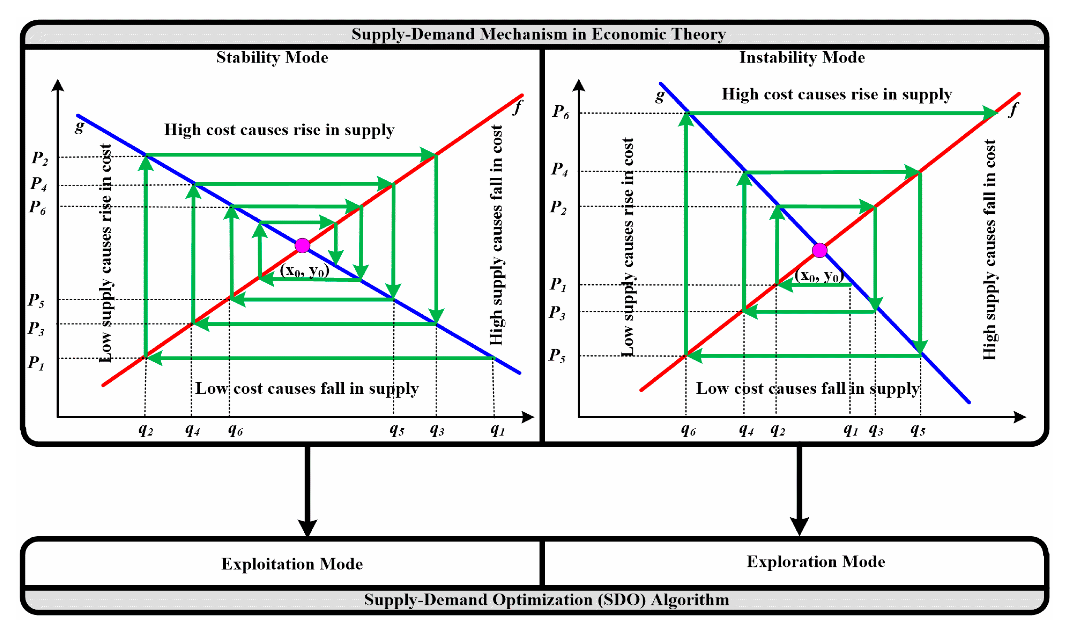
3.1. Preliminary Concepts

The SDO replicates the consumer–producer supply–demand relationship [34]. Economic principles dictate that the quantity and cost of a commodity are determined by its current cost and quantity in the market, respectively. When the market’s current cost of a product falls, the amount of that commodity provided increases. By contrast, as a commodity’s supply grows, its market price drops. After a period of time, the quantity and cost reach a point of balance (x0, y0). The supply–demand strategy has the following two distinct modes: stable and instable (Figure 2). The cost and quantity congregate at a balancing point in the stable mode, which may be applied to SDO as exploitation to conduct a local pursuit. In the instable mode, the cost and quantity vary from the equilibrium point and may be matched to SDO as exploration to conduct a global search in the search region [48].

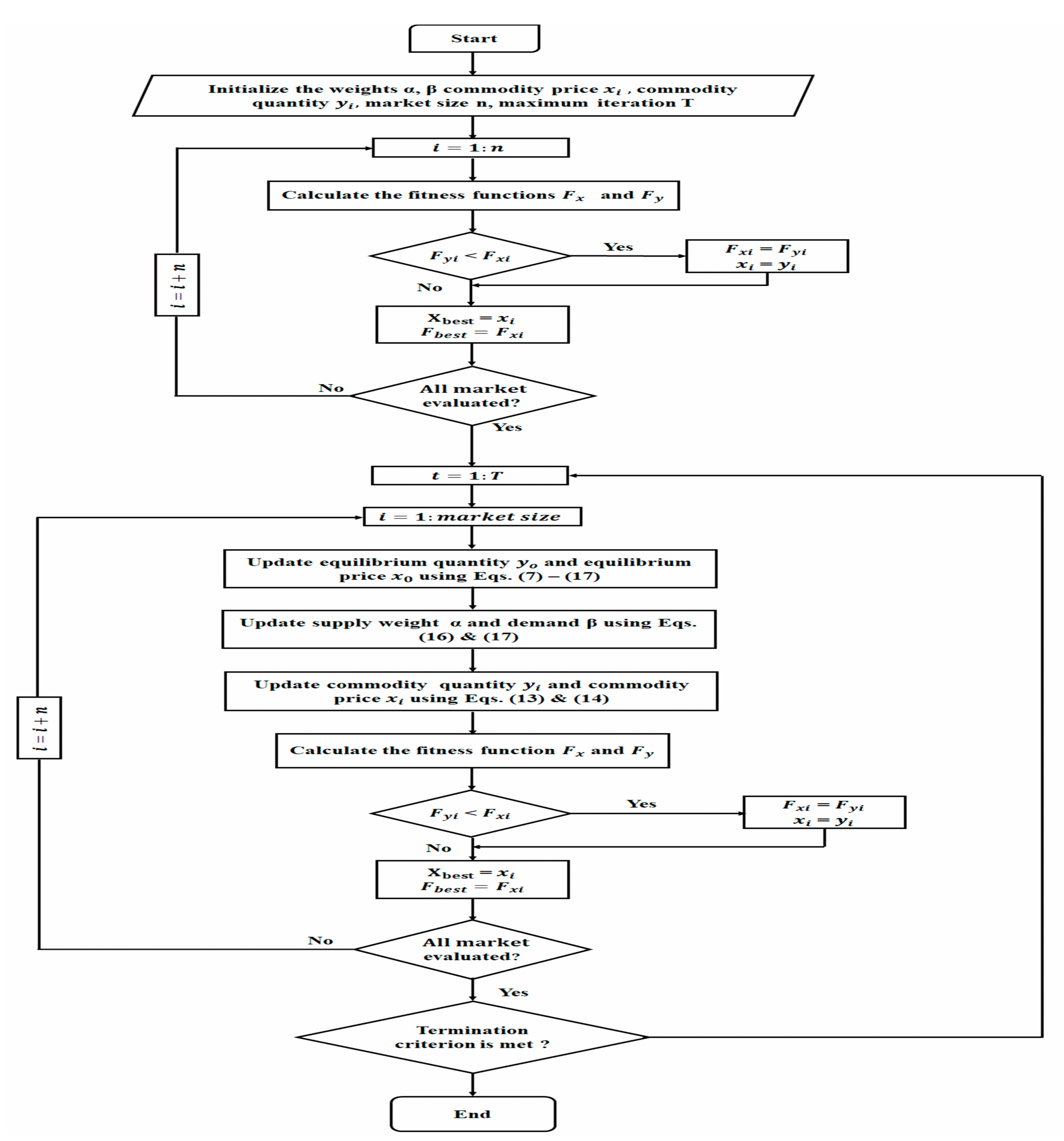
3.2. Supply–Demand-Based Optimization (SDO) Algorithm

The SDO is predicated on the existence of n markets, each of which contains d commodities. Each commodity is limited in quantity and has a particular cost. The market’s commodity cost and quantity are expressed as follows:

$$X=\left[\begin{array}{c}{x}_1\\ x_2\\ \begin{array}{c}⋮\\ x_n\end{array}\end{array}\right]=\left[\begin{array}{c}\begin{array}{ccc}{x}_1^1& \begin{array}{cc}{x}_1^2& \dots \end{array}& x_1^d\end{array}\\ \begin{array}{ccc}{x}_2^1& \begin{array}{cc}{x}_2^2& \dots \end{array}& x_2^d\end{array}\\ \begin{array}{c}\begin{array}{ccc}\begin{array}{cc}⋮ & ⋮\end{array}& ⋮& ⋮\end{array} \\ \begin{array}{ccc}{x}_n^1& \begin{array}{cc}{x}_n^2& \dots \end{array}& x_n^d\end{array}\end{array}\end{array}\right]$$

(17)

$$Y=\left[\begin{array}{c}{y}_1\\ y_2\\ \begin{array}{c}⋮\\ y_n\end{array}\end{array}\right]={\left[\begin{array}{c}\begin{array}{ccc}{y}_1^1& \begin{array}{cc}{y}_1^2& \dots \end{array}& y_1^d\end{array}\\ \begin{array}{ccc}{y}_2^1& \begin{array}{cc}{y}_2^2& \dots \end{array}& y_2^d\end{array}\\ \begin{array}{c}\begin{array}{ccc}\begin{array}{cc}⋮ & ⋮\end{array}& ⋮& ⋮\end{array} \\ \begin{array}{ccc}{y}_n^1& \begin{array}{cc}{y}_n^2& \dots \end{array}& y_n^d\end{array}\end{array}\end{array}\right]}_{ }$$

(18)

where $x_i^j$ (i = 1, …,n; j = 1,…, d) and $y_i^j$ (i = 1,…, n; j = 1, …d) denote the ^jth cost and ^jth quantity, respectively, of a commodity in the ⁱth market; n denotes the number of markets; and d denotes the number of commodity costs and commodity quantities in each market.

The commodity cost and quantity are determined for each market by inputting the decision variable values into the fitness function.

$$\left[\begin{array}{c}{F}_x\\ F_y\end{array}\right]=\left[\begin{array}{c}\begin{array}{ccc}{F}_{x1}& \begin{array}{cc}{F}_{x2}& \dots \end{array}& F_{xn}\end{array}\\ \begin{array}{ccc}{F}_{y1}& \begin{array}{cc}{F}_{y2}& \dots \end{array}& F_{yn}\end{array}\end{array}\right]$$

(19)

The modified cost and quantity are then evaluated using the objective function. If the value of the commodity quantities’ fitness function is less than that of its cost, its cost will be swapped with its commodity quantity as a potential solution.

To prevent SDO from being trapped in a local optima, the balance cost $y_0$ and balance quantity vector $x_0$ are chosen at random, as shown in [48].

$$N_i=\left|F_{yi}-\frac{1}{n}\sum _{i=1}^n{F}_{yi}\right|$$

(20)

$$Q=\frac{N_i}{{\sum }_{i=1}^n{N}_i}$$

(21)

$$y_0=y_k, k=Roulette wheel selection \left(Q\right)$$

(22)

$$M_i=\left|F_{xi}-\frac{1}{n}\sum _{i=1}^n{F}_{xi}\right|$$

(23)

$$P=\frac{M_i}{{\sum }_{i=1}^n{M}_i}$$

(24)

$$x_0=\{\begin{array}{ll}{r}_1·\frac{{\sum }_{i=1}^n{x}_i}{n}& if rand<0.5\\ x_k, k=Roulette wheel selection \left(P\right)& if rand\ge 0.5\end{array}$$

(25)

where r₁ is a random number.

By changing the supply $\alpha$ and demand $\beta$ constants, the subsequent commodity quantity and commodity cost are updated based on the equilibrium cost and equilibrium quantity, respectively.

$$y_i\left(t+1\right)=y_0+\alpha ·\left(x_i\left(t\right)-x_0\right)$$

(26)

$$x_i\left(t+1\right)=x_0+\beta ·\left(y_i\left(t+1\right)-y_0\right)$$

(27)

where $x_i$ and $y_i$denote the ⁱth cost and quantity of a commodity at the $t$th iteration, respectively.

The commodity cost may be expressed as follows, using (26) and (27):

$$x_i\left(t+1\right)=x_0+\alpha \beta ·\left(x_i\left(t\right)-x_0\right)$$

(28)

To achieve a balance between exploration and exploitation, $\alpha , \beta$ are expressed as follows:

$$\alpha =\frac{2\left(T-t+1\right)}{T}\sin \left(2\pi r\right) \mathrm{and} \beta =2\cos \left(2\pi r\right)$$

(29)

where T is the maximum number of iterations, t is the current iteration, r is a random value, and t is the current iteration.

To aid the SDO in quickly transitioning between exploration and exploitation, a new variable L is defined as follows:

$$L=\alpha \beta =\frac{4\left(T-t+1\right)}{T}\sin \left(2\pi r\right)\cos \left(2\pi r\right)$$

(30)

For each market, the commodity cost diverges from the balance cost when $\left|L\right|>1$ and converges to the balance cost when $\left|L\right|<1$. The SDO is depicted in Figure 3.

4. Experimental Results and Discussion

This section demonstrates the effectiveness of the SDO algorithm in estimating the optimal parameters of PEMFC stacks, by an analysis of the SDO algorithm under various operating and design parameters. The optimization processes are executed using MATLAB-R2019a (version 9.6) under Windows 7 Pro 64-bit with an Intel^® Core i7 CPU @ 2.8 GHz and 8 MB RAM.

Two cases were investigated, so that the superiority/competitiveness of the proposed SDO-based process was confirmed. The first case presents the achieved results related to different operational conditions of the PEMFC stack, whereas the second case presents the results for two well-known PEMFCs stacks, BSC500W and 500W Horizon. The SDO algorithm was also compared with five algorithms that were used in the literature, to evaluate its performance in estimating PEMFC stack parameters. Nine parameters (${\xi }_1, {\xi }_2, {\xi }_3, {\xi }_4, R_c, \beta , \lambda , l, \mathrm{and} J_{max}$) were optimized, and the maximum and minimum constraints of these parameters are listed in

Table 1. Upper and lower constraints of the PEMFC parameters [49].

Parameter	Constraints
	Upper	Lower
${\xi }_1$	−0.8532	−1.19969
${\xi }_2$	5.00 × 10−3	1.00 × 10−3
${\xi }_3$	9.8 × 10−5	3.6 × 10−5
${\xi }_4$	−9.54 × 10−5	−260 × 10−4
$R_c$ (Ω)	8.00 × 10−4	1.00 × 10−4
$\beta$ (V)	0.5	0.0136
$\lambda$	24	10
$l \left(\mu m\right)$	178	51
$J_{max} \left(mA\right)$	1500	850

. It is worth mentioning that the optimal parameters, after 50 independent runs of each algorithm, were statistically evaluated and the best result was then selected from these runs.

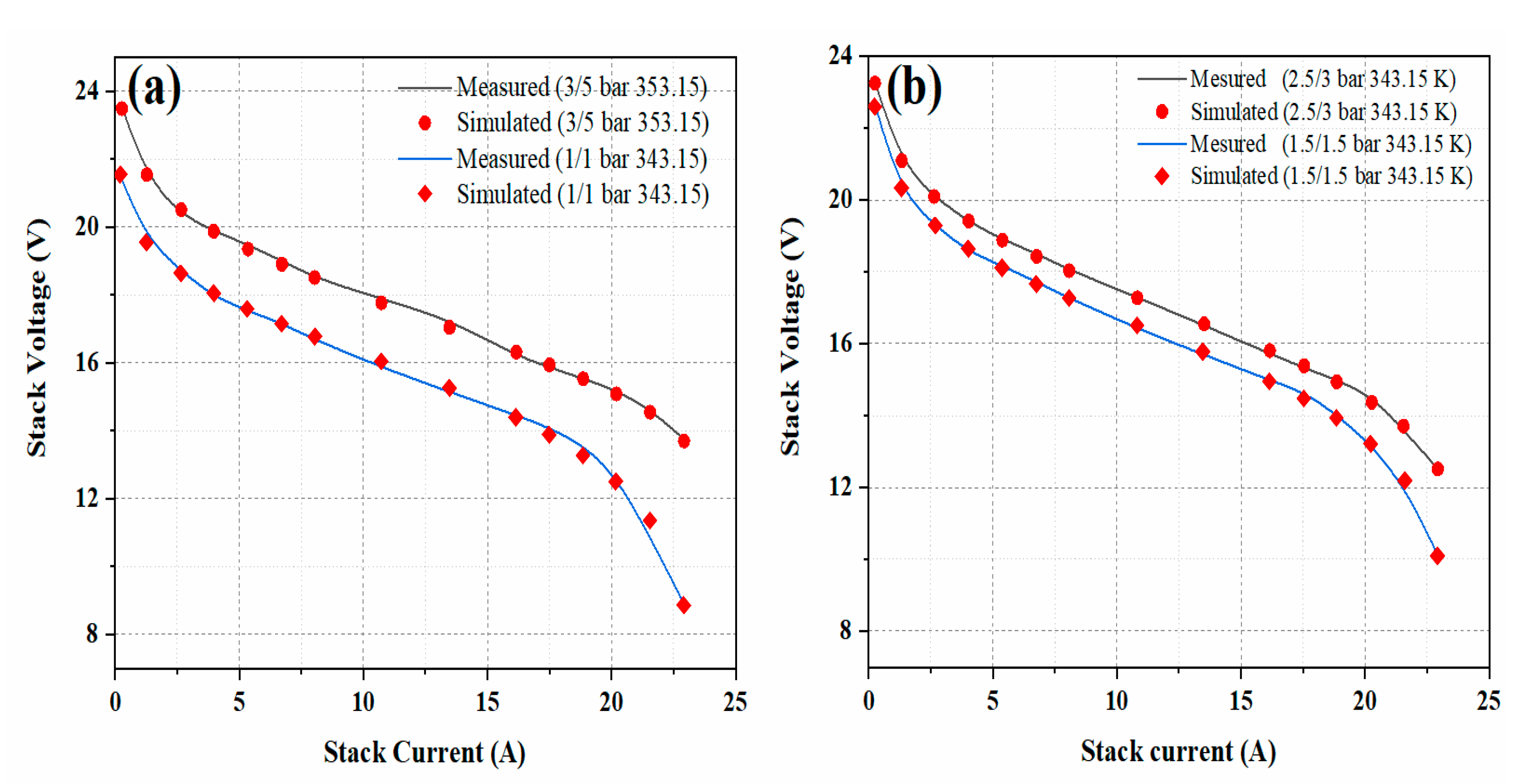
4.1. Case Study 1 (Different Operational Conditions)

In this case, the supremacy of the SDO algorithm was evaluated using the experimental data that are shown in

Table A1. The experiment data used for case 1 [47].

No.	3/5 bar 353.15 K		1/1 bar 343.15 K		2.5/3 bar 343.15 K		1.5/1.5 bar 343.15 K
	Current (A)	Voltage (V)	Current (A)	Voltage (V)	Current (A)	Voltage (V)	Current (A)	Voltage (V)
1	0.2729	23.5410	0.2046	21.5139	0.2582	23.2710	0.2417	22.6916
2	1.2790	21.4756	1.2619	19.6737	1.3340	21.0280	1.3177	20.1869
3	2.6603	20.3484	2.6433	18.7154	2.6471	20.0748	2.6819	19.2897
4	3.9734	19.8969	3.9734	17.9449	4.0281	19.4019	4.0118	18.5607
5	5.3547	19.4642	5.3206	17.5497	5.3919	18.8972	5.3755	18.1682
6	6.7190	19.0127	6.7019	17.1545	6.7726	18.5047	6.7563	17.7196
7	8.0321	18.5049	8.0491	16.6843	8.0852	18.0561	8.0689	17.2710
8	10.7265	17.8835	10.7265	15.8752	10.8297	17.2897	10.8134	16.4299
9	13.4720	17.2808	13.4720	15.1411	13.5230	16.5047	13.4556	15.7009
10	16.1664	16.2089	16.1494	14.4634	16.1652	15.7196	16.1488	14.9907
11	17.4966	15.8701	17.4795	14.0870	17.5459	15.3271	17.5295	14.6542
12	18.8608	15.5312	18.8438	13.5792	18.8584	14.9907	18.8423	14.0374
13	20.1910	15.1923	20.1739	12.6772	20.2733	14.5421	20.2234	13.1963
14	21.5553	14.6282	21.5382	10.8743	21.5523	13.5888	21.6049	12.0187
15	22.9195	13.7450	22.9025	8.92130	22.9337	12.5234	22.9189	10.1308

(in the Appendix A). Four different sets of measured data were used; two sets (3/5 bar 353.15 K, 1/1 bar 343.15 K) were used to extract the PEMFC parameters, and the other sets (2.5/3 bar 343.15 K, 1.5/1.5 bar 343.15 K) were used in model validation. The operational ranges and the known parameters that were used in this study, are listed in

Table 2. Known parameters the PEMFC stack [49].

Parameter	Value	Parameter	Value
n	24	Pa (bar)	1.0–3.0
A (cm2)	27	Pb (bar)	1.0–5.0
Power (w)	250	RHa	1.0
T(K)	343.15–353.15	RHb	1.0

. The I–V curves of the PEMFC stacks, along with the finest parameter values that were obtained by the SDO algorithm, are plotted in Figure 4. It is obvious that the simulated and experimental I–V curves agree well, regardless of the experimental data that were used for model validation or the experimental data that were used for parameter estimation.

After executing the SDO to identify the optimal values of the nine unknown parameters, the best values of the identified PEMFC model, using five well-known algorithms (WOA, GWO, SSA, HHO, and GA), were identified (

Table 3. The SSE statistical results achieved by the six algorithms (2.5/3 bar, 343.15 K).

SSE	Optimization Algorithms
	WOA	GWO	SSA	HHO	GA	SDO
Minimum	0.154639186	0.146884822	0.152883434	0.167631296	0.350360131	0.145167469
Mean	0.419153062	0.170258026	0.178072981	0.491306301	1.561131011	0.148407841
Median	0.397898527	0.157920235	0.155409751	0.424590144	1.360612054	0.147780145
Maximum	1.073495308	0.346056858	0.419199433	1.288663305	7.448856801	0.154441127
STD	0.196771275	0.033980005	0.062370696	0.262778766	1.266038132	0.002718387

and

Table 4. Optimal parameters achieved by the six algorithms (2.5/3 bar, 343.15 K).

Variable	Algorithm
	WOA	GWO	SSA	HHO	GA	SDO
${\xi }_1$	−0.884007645	−0.944234024	−1.07199885	−1.156237962	−0.90822	−0.964599939
${\xi }_2$	0.002484898	0.002893255	0.002880452	0.002958249	0.00295	0.002440458
${\xi }_3$	6.06253 × 10−5	7.86346 × 10−5	4.99592 × 10−5	3.73411 × 10−5	0.00009	3.96338 × 10−5
${\xi }_4$	−0.000139704	−0.000137972	−0.000137754	−0.000144177	−0.00013	−0.000138061
$R_c$	0.000178974	0.000172751	0.000158811	0.000559279	0.00045	0.000100003
$\beta$	0.051607571	0.019026091	0.026518418	0.016646806	0.089330	0.015471
$\lambda$	16.02236023	10.46643873	15.5096387	10.00002765	12.14717	10.00039
$l$	0.008914346	0.010066463	0.014396789	0.008537823	0.00815	0.010209
$J_{max}$	0.939531061	0.873824589	0.886530415	0.864155406	1.27485	0.86617
$SSE$	0.154639186	0.146884822	0.152883434	0.167631296	0.350360131	0.145167

). To statistically assess all of the algorithms, the following five statistical indicators were calculated: mean, median, standard deviation, maximum, and lowest indices of best-so-far solutions over all 50 separate runs. The best results are presented in bold text to simplify their readability. According to recent reports, these five algorithms can solve this problem well; for this reason, they were chosen for comparison in this study.

All the parameters for each algorithm were set to the same values, to allow for a fair comparison. As per the results of these tables, it is evident that SDO is able to outperform other algorithms in terms of all the statistical indicators. When compared to the effectiveness of the WOA, GWO, SSA, HHO, and GA, in terms of the “STD” indicator, SDO outperforms them all. The SDO’s low STD value indicates that it converged in the majority of the trials, showing its robustness.

4.2. Case Study 2 (Different Types of PEMFC Stacks)

4.2.1. BCS-500W

In this case, a BCS PEMFC stack, manufactured by the American Company BCS Technologies, with 500 W, was used to examine the performance of the SDO algorithm. The characteristics of this BCS PEMFC were reported by Ali M et al. [19], as follows: N_cell = 32, A = 64 cm², T_stack = 333 K, PH₂ = 1 atm, and PO₂ = 0.2075 atm. The dataset measurements I/V (reported in

Table A2. The experiment data of BCS-500W PEMFC stack [33].

No.	Current (A)	Voltage (V)	No.	Current (A)	Voltage(V)
1	0.60	29	10	15.73	21.09
2	2.10	26.31	11	17.02	20.68
3	3.58	25.09	12	19.11	20.22
4	5.08	24.25	13	21.20	19.76
5	7.17	23.37	14	23.00	19.36
6	9.55	22.57	15	25.08	18.86
7	11.35	22.06	16	27.17	18.27
8	12.54	21.75	17	28.06	17.95
9	13.73	21.45	18	29.26	17.30

in the Appendix A) of the BCS 500-W PEMFC stack were utilized to optimize nine unknown parameters, using the SDO algorithm as well as the other five algorithms that were mentioned previously, for comparison.

Table 5. The SSE statistical results achieved by the six algorithms (BCS-500W).

SSE	Algorithms
	WOA	GWO	SSA	HHO	GA	SDO
Minimum	0.300165193	0.295994285	0.309587261	0.29652213	0.699327274	0.287824529
Mean	0.577755836	0.377546219	0.399386254	0.936986404	2.553703279	0.291280092
Median	0.463634598	0.371127461	0.40787451	0.544159818	2.515251534	0.290517966
Maximum	2.037256664	0.458303674	0.456663355	2.774235022	6.340709893	0.300122801
STD	0.305965318	0.04832738	0.040168552	0.736897544	1.213128222	0.003306558

presents the SSE results that were obtained by the different algorithms. Consistent with Table 5, the smallest SSE values were achieved by the SDO algorithm, as compared with the other algorithms, i.e., the results show that the SDO algorithm was able to improve the previous best SSE value.

Table 6. Optimal parameters achieved by the six algorithms (BCS-500W).

Variable	Algorithms
	WOA	GWO	SSA	HHO	GA	SDO
${\xi }_1$	−0.9715	−0.890402371	−0.935709319	−1.188920972	−0.971500	−1.108875289
${\xi }_2$	0.00251	0.002491237	0.003094492	0.003832179	0.002510	0.00344834
${\xi }_3$	0.000036	4.91 × 10−5	7.92 × 10−5	7.78 × 10−5	0.000036	6.85 × 10−5
${\xi }_4$	−0.00015	−0.000178916	−0.000178501	−0.000177945	−0.000150	−0.00018002
$R_c$	0.00047	0.000185305	0.000125487	0.000100056	0.000470	0.000100079
$\beta$	0.24611	0.128317025	0.116173722	0.132384143	0.246110	0.133014223
$\lambda$	15.32527	21.56036185	19.20514021	19.76775546	15.32527	23.99819531
$l$	0.00807	0.005306549	0.008197421	0.005272008	0.008070	0.005101562
$J_{max}$	1.40447	0.85	0.85	0.850476147	1.404470	0.850000467
$SSE$	0.699327274	0.295994285	0.309587261	0.29652213	0.699327274	0.287824529

shows that the algorithms that were used in this case study successfully extracted the nine parameters.

4.2.2. Horizon-500W

An open-cathode Horizon PEMFC, with a nominal power of 500 W, was used to validate the performance of the SDO. The operating details for this PEMFC can be found in Refs. [33,54], and its features are as follows: N_cell = 36, A = 52 cm², T_stack = 333 K, PH₂ = 0.55 atm, and PO₂ = 1 atm.

The current vs. voltage datasets that were utilized to validate the SDO-determined optimal PEMFC stack parameters, are presented in

Table A3. The experiment data of Horizon-500W PEMFC stack [33].

No.	Current (A)	Voltage (V)
1	0.6	29.370000
2	2.5	26.777390
3	5	25.290250
4	7.5	24.281859
5	10	23.418000
6	12	22.739103
7	14	22.058523
8	16	21.386148
9	18	20.721728
10	20	20.026000
11	21	19.636350
12	22	19.191807
13	23	18.663630
14	24	18.015227
15	25	17.201250

. To assess the SDO results, comparisons with other algorithm methods were performed, as shown in

Table 7. The SSE statistical results achieved by the six algorithms (Horizon-500W).

SSE	Algorithm
	WOA	GWO	SSA	HHO	GA	SDO
Minimum	0.625844193	0.573184966	0.57403609	0.615881844	0.819730928	0.56426671
Mean	1.061565396	0.636443826	0.736015304	1.896482889	1.628325244	0.567576781
Median	1.011063049	0.619793268	0.697756101	0.788884976	1.395475534	0.565250928
Maximum	4.841737291	0.887128302	0.952794404	10.23959957	4.949883945	0.58254602
STD	0.559655929	0.065968875	0.108664932	2.287173428	0.810383099	0.004466494

. As per the tabulated values, SDO gave the best SSE value among all the optimizers. The performance test measures and numerical comparisons with the other optimizers noticeably highlight that the SDO was best able to optimize the nine unknown PEMFC model parameters.

Table 8. Best optimized parameters of Horizon-500W PEMFC stack achieved by the six algorithms.

Variable	Algorithm
	WOA	GWO	SSA	HHO	GA	SDO
${\xi }_1$	−1.199166641	−0.887481442	−1.155052815	−0.854760973	−0.975720	−0.902401475
${\xi }_2$	0.003060175	0.002252875	0.003202954	0.001875009	0.003110	0.002101847
${\xi }_3$	4.64 × 10−5	5.56 × 10−5	6.62 × 10−5	3.60 × 10−5	0.000098	4.16 × 10−5
${\xi }_4$	−0.000109916	−0.000112573	−0.00011186	−0.000106249	−0.000100	−0.000112065
$R_c$	0.000100072	0.000119116	0.000101536	0.000100031	0.000550	0.000100019
$\beta$	0.160910761	0.195372815	0.194323477	0.177260104	0.220680	0.199832662
$\lambda$	10.01525068	21.55450995	18.31630737	10.003083	18.90174	23.995893
$l$	0.006712446	0.00554807	0.0051	0.005101572	0.011480	0.005100055
$J_{max}$	0.85106307	0.85	0.85	0.850262055	1.017500	0.850000594
$SSE$	0.625844193	0.573184966	0.57403609	0.615881844	0.819730928	0.56426671

compares the parameter values and minimum SSE values for the PEMFC stack with those given by the other algorithms. As shown in Table 8, the method precision and advantages of the SDO algorithm are greater than those for the other algorithms.

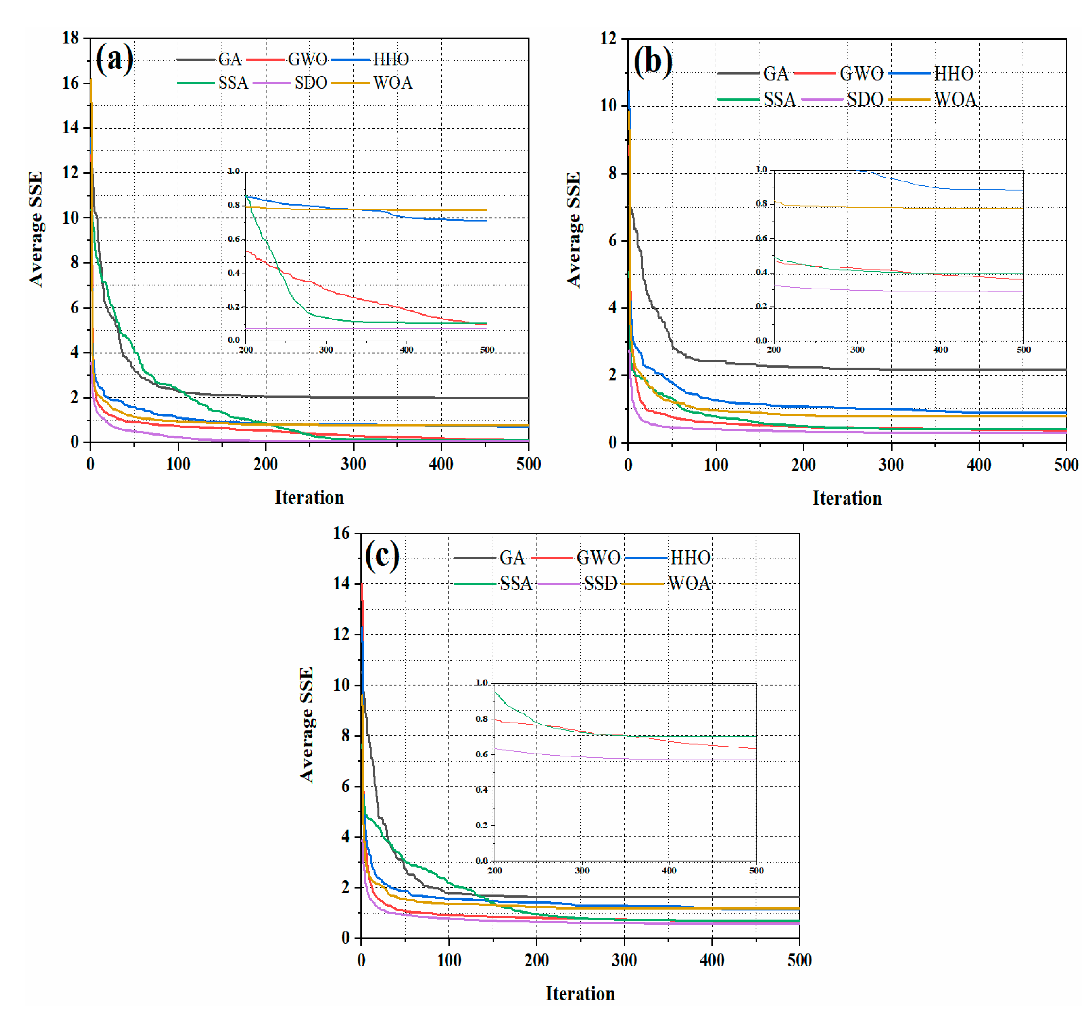
4.3. Average Convergence Rate

Under the same operating conditions that were used for the three above-mentioned PEMFC stacks, the average convergence curves of the best SSE values of 50 runs that were generated by SDO, WOA, GWO, SSA, HHO, and GA, are shown in Figure 5. It can be observed from Figure 5 that in the first 100 iterations, the average convergence rate of the first three algorithms followed the following order: SDO > GWO > WOA. In later iterations, the inset (zoomed-in portion) of Figure 5 indicates that their convergence rate follows the following order: SDO > GWO > SSA. Indeed, for the whole optimization process, the SDO algorithm has the fastest rate of convergence and the highest SSE accuracy when compared with WOA, GWO, SSA, HHO, and GA. This supremacy can be attributed to the algorithm architecture that was discussed in Section 3.

5. Conclusions

A novel design methodology, based on a newly proposed computational intelligence algorithm, named SDO, to identify the parameters of three PEMFC stacks under different operating conditions, is proposed. A comparison of SDO with the WOA, GWO, SSA, HHO, and GA algorithms is accomplished by considering the SSE between the measured and calculated voltage for three PEMFC stacks over 50 independent runs. In this regard, the following nine estimated variables were considered$: {\xi }_1, {\xi }_2, {\xi }_3, {\xi }_4, R_c, \beta , \lambda , l, \mathrm{and} J_{max}$. The investigation was experimentally implemented on the following different PEMFC stacks: 250W stack, BCS-500W, and Horizon-500W. It was assumed that the relative humidity at the anode and cathode sides was 100% for all the PEMFCs. The optimization results validate the supremacy and reliability of the SDO algorithm over the other algorithms, in terms of extracting the optimal parameters of PEMFC stacks under different conditions. SDO converged rapidly towards the optimum solutions for the three PEMFCs stacks; this was not the case for the other algorithms, particularly for GA, which diverged significantly. Moreover, the achieved STD of SDO was markedly lower than that for the other algorithms, highlighting the reason for the accuracy and repeatability of the SDO algorithm. Utilization of the SDO algorithm in dynamic PEMFC model identification, as well as the investigation of new algorithms, are suggestions for further work.

References

1. Al-Shamma’a, A.A.; Addoweesh, K.E. Techno-economic optimization of hybrid power system using genetic algorithm. Int. J. Energy Res. 2014, 38, 1608–1623. [Google Scholar] [CrossRef]
2. Uzunoglu, M.; Alam, M.S. Fuel-Cell Systems for Transportations; Elsevier BV: Amsterdam, The Netherlands, 2018; pp. 1091–1112. [Google Scholar]
3. Ghasemi, M.; Shahgaldi, S.; Ismail, M.; Yaakob, Z.; Daud, W.R.W. New generation of carbon nanocomposite proton exchange membranes in microbial fuel cell systems. Chem. Eng. J. 2012, 184, 82–89. [Google Scholar] [CrossRef]
4. Jia, J.; Wang, Y.; Li, Q.; Cham, Y.T.; Han, M. Modeling and Dynamic Characteristic Simulation of a Proton Exchange Membrane Fuel Cell. IEEE Trans. Energy Convers. 2009, 24, 283–291. [Google Scholar] [CrossRef]
5. Massonnat, P.; Gao, F.; Roche, R.; Paire, D.; Bouquain, D.; Miraoui, A. Multiphysical, multidimensional real-time PEM fuel cell modeling for embedded applications. Energy Convers. Manag. 2014, 88, 554–564. [Google Scholar] [CrossRef]
6. Soltani, M.; Bathaee, S.M.T. Development of an empirical dynamic model for a Nexa PEM fuel cell power module. Energy Convers. Manag. 2010, 51, 2492–2500. [Google Scholar] [CrossRef]
7. Gao, F.; Blunier, B.; Miraoui, A. (Eds.) Proton Exchange Membrane Fuel Cells Modeling; John Wiley & Sons Inc.: Hoboken, NJ, USA, 2012. [Google Scholar]
8. Secanell, M.; Wishart, J.; Dobson, P. Computational design and optimization of fuel cells and fuel cell systems: A review. J. Power Sources 2011, 196, 3690–3704. [Google Scholar] [CrossRef]
9. Secanell, M.; Carnes, B.; Suleman, A.; Djilali, N. Numerical optimization of proton exchange membrane fuel cell cathodes. Electrochim. Acta 2007, 52, 2668–2682. [Google Scholar] [CrossRef]
10. Mohammadi, A.; Cirrincione, G.; Djerdir, A.; Khaburi, D.A. A novel approach for modeling the internal behavior of a PEMFC by using electrical circuits. Int. J. Hydrogen Energy 2018, 43, 11539–11549. [Google Scholar] [CrossRef]
11. Lin, H.-H.; Cheng, C.-H.; Soong, C.-Y.; Chen, F.; Yan, W.-M. Optimization of key parameters in the proton exchange membrane fuel cell. J. Power Sources 2006, 162, 246–254. [Google Scholar] [CrossRef]
12. Youssef, M.; Elsal-Nadi, K.E.; Khalil, M.H. Lumped model for proton exchange membrane fuel cell (PEMFC). Int. J. Electrochem. Sci. 2010, 5, 267–277. [Google Scholar]
13. Jiang, Y.; Yang, Z.; Jiao, K.; Du, Q. Sensitivity analysis of uncertain parameters based on an improved proton exchange membrane fuel cell analytical model. Energy Convers. Manag. 2018, 164, 639–654. [Google Scholar] [CrossRef]
14. Amirinejad, M.; Rowshanzamir, S.; Eikani, M.H. Effects of operating parameters on performance of a proton exchange membrane fuel cell. J. Power Sources 2006, 161, 872–875. [Google Scholar] [CrossRef]
15. Yang, X.-S. Review of meta-heuristics and generalised evolutionary walk algorithm. Int. J. Bio-Inspired Comput. 2011, 3, 77. [Google Scholar] [CrossRef]
16. Mohamed, I.; Jenkins, N. Proton exchange membrane (PEM) fuel cell stack configuration using genetic algorithms. J. Power Sources 2004, 131, 142–146. [Google Scholar] [CrossRef]
17. Askarzadeh, A.; Rezazadeh, A. Optimization of PEMFC model parameters with a modified particle swarm optimization. Int. J. Energy Res. 2010, 35, 1258–1265. [Google Scholar] [CrossRef]
18. Zhang, G.; Xiao, C.; Razmjooy, N. Optimal parameter extraction of PEM fuel cells by meta-heuristics. Int. J. Ambient. Energy 2020, 2020, 1–10. [Google Scholar] [CrossRef]
19. Ali, M.; El-Hameed, M.; Farahat, M. Effective parameters’ identification for polymer electrolyte membrane fuel cell models using grey wolf optimizer. Renew. Energy 2017, 111, 455–462. [Google Scholar] [CrossRef]
20. Outeiro, M.; Chibante, R.; Carvalho, A.; de Almeida, A. A parameter optimized model of a Proton Exchange Membrane fuel cell including temperature effects. J. Power Sources 2008, 185, 952–960. [Google Scholar] [CrossRef]
21. Askarzadeh, A.; Rezazadeh, A. An Innovative Global Harmony Search Algorithm for Parameter Iden-tification of a PEM Fuel Cell Model. IEEE Trans. Ind. Electron. 2012, 59, 3473–3480. [Google Scholar] [CrossRef]
22. Askarzadeh, A.; Rezazadeh, A. A new artificial bee swarm algorithm for optimization of proton ex-change membrane fuel cell model parameters. J. Zhejiang Univ. Sci. C 2011, 12, 638–646. [Google Scholar] [CrossRef]
23. Priya, K.; Rajasekar, N. Application of flower pollination algorithm for enhanced proton exchange membrane fuel cell modelling. Int. J. Hydrogen Energy 2019, 44, 18438–18449. [Google Scholar] [CrossRef]
24. Zhang, W.; Wang, N.; Yang, S. Hybrid artificial bee colony algorithm for parameter estimation of proton exchange membrane fuel cell. Int. J. Hydrogen Energy 2013, 38, 5796–5806. [Google Scholar] [CrossRef]
25. Sedighizadeh, M.; Mahmoodi, M.M.; Soltanian, M. Parameter identification of proton exchange membrane fuel cell using a Hybrid Big Bang-Big Crunch optimization. In Proceedings of the 2014 5th Conference on Thermal Power Plants (lPGC2014), Tehran, Iran, 10–11 June 2014; pp. 35–39. [Google Scholar]
26. El-Fergany, A.A. Extracting optimal parameters of PEM fuel cells using Salp Swarm Optimizer. Renew. Energy 2018, 119, 641–648. [Google Scholar] [CrossRef]
27. Han, W.; Li, D.; Yu, D.; Ebrahimian, H. Optimal parameters of PEM fuel cells using chaotic binary shark smell optimizer. Energy Sources Part A Recover. Util. Environ. Eff. 2019, 2019, 1–15. [Google Scholar] [CrossRef]
28. Fathy, A.; Rezk, H. Multi-verse optimizer for identifying the optimal parameters of PEMFC model. Energy 2018, 143, 634–644. [Google Scholar] [CrossRef]
29. Guo, C.; Lu, J.; Tian, Z.; Guo, W.; Darvishan, A. Optimization of critical parameters of PEM fuel cell using TLBO-DE based on Elman neural network. Energy Convers. Manag. 2019, 183, 149–158. [Google Scholar] [CrossRef]
30. Khan, S.S.; Rafiq, M.A.; Shareef, H.; Sultan, M.K. Parameter optimization of PEMFC model using back-tracking search algo-rithm. In Proceedings of the 2018 5th International Conference on Renewable Energy: Generation and Applications (ICREGA), Al Ain, United Arab Emirates, 25–28 February 2018; pp. 323–326. [Google Scholar]
31. Sun, Z.; Wang, N.; Bi, Y.; Srinivasan, D. Parameter identification of PEMFC model based on hybrid adaptive differential evolution algorithm. Energy 2015, 90, 1334–1341. [Google Scholar] [CrossRef]
32. Niu, Q.; Zhang, L.; Li, K. A biogeography-based optimization algorithm with mutation strategies for model parameter es-timation of solar and fuel cells. Energy Convers. Manag. 2014, 86, 1173–1185. [Google Scholar] [CrossRef]
33. Kandidayeni, M.; Macias, A.; Khalatbarisoltani, A.; Boulon, L.; Kelouwani, S. Benchmark of proton ex-change membrane fuel cell parameters extraction with metaheuristic optimization algorithms. Energy 2019, 183, 912–925. [Google Scholar] [CrossRef]
34. El-Fergany, A.A. Electrical characterisation of proton exchange membrane fuel cells stack using grasshopper optimiser. IET Renew. Power Gener. 2018, 12, 9–17. [Google Scholar] [CrossRef]
35. Askarzadeh, A.; Rezazadeh, A. A new heuristic optimization algorithm for modeling of proton ex-change membrane fuel cell: Bird mating optimizer. Int. J. Energy Res. 2013, 37, 1196–1204. [Google Scholar] [CrossRef]
36. El-Fergany, A.A.; Hasanien, H.M.; Agwa, A.M. Semi-empirical PEM fuel cells model using whale optimization algorithm. Energy Convers. Manag. 2019, 201, 112197. [Google Scholar] [CrossRef]
37. Duan, B.; Cao, Q.; Afshar, N. Optimal parameter identification for the proton exchange membrane fuel cell using Satin Bowerbird optimizer. Int. J. Energy Res. 2019. [Google Scholar] [CrossRef]
38. Cao, Y.; Li, Y.; Zhang, G.; Jermsittiparsert, K.; Razmjooy, N. Experimental modeling of PEM fuel cells using a new improved seagull optimization algorithm. Energy Rep. 2019, 5, 1616–1625. [Google Scholar] [CrossRef]
39. Fathy, A.; Elaziz, M.A.; Alharbi, A.G. A novel approach based on hybrid vortex search algorithm and differential evolution for identifying the optimal parameters of PEM fuel cell. Renew. Energy 2020, 146, 1833–1845. [Google Scholar] [CrossRef]
40. Turgut, O.E.; Coban, M.T. Optimal proton exchange membrane fuel cell modelling based on hybrid Teaching Learning Based Optimization—Differential Evolution algorithm. Ain Shams Eng. J. 2016, 7, 347–360. [Google Scholar] [CrossRef]
41. Kamel, S.; Jurado, F.; Sultan, H.M.; Menesy, A.S. Tree Growth Algorithm for Parameter Identification of Proton Exchange Membrane Fuel Cell Models. Int. J. Interact. Multimed. Artif. Intell. 2020, 6, 11. [Google Scholar] [CrossRef] [Green Version]
42. Menesy, A.S.; Sultan, H.M.; Selim, A.; GAshmawy, M.; Kamel, S. Developing and Applying Chaotic Harris Hawks Optimization Technique for Extracting Parameters of Several Proton Exchange Membrane Fuel Cell Stacks. IEEE Access 2020, 8, 1146–1159. [Google Scholar] [CrossRef]
43. Agwa, A.M.; El-Fergany, A.A.; Sarhan, G.M. Steady-State Modeling of Fuel Cells Based on Atom Search Optimizer. Energies 2019, 12, 1884. [Google Scholar] [CrossRef] [Green Version]
44. Isa, Z.M.; Nayan, N.M.; Arshad, M.H.; Kajaan, N.A.M. Optimizing PEMFC model parameters using ant li-on optimizer and dragonfly algorithm: A comparative study. Int. J. Electr. Comput. Eng. 2019, 9, 5295. [Google Scholar]
45. Chen, Y.; Wang, N. Cuckoo search algorithm with explosion operator for modeling proton exchange membrane fuel cells. Int. J. Hydrogen Energy 2019, 44, 3075–3087. [Google Scholar] [CrossRef]
46. Askarzadeh, A.; Rezazadeh, A. Artificial immune system-based parameter extraction of proton exchange membrane fuel cell. Int. J. Electr. Power Energy Syst. 2011, 33, 933–938. [Google Scholar] [CrossRef]
47. Xu, S.; Wang, Y.; Wang, Z. Parameter estimation of proton exchange membrane fuel cells using eagle strategy based on JAYA algorithm and Nelder-Mead simplex method. Energy 2019, 173, 457–467. [Google Scholar] [CrossRef]
48. Zhao, W.; Wang, L.; Zhang, Z. Supply-Demand-Based Optimization: A Novel Economics-Inspired Algorithm for Global Optimization. IEEE Access 2019, 7, 73182–73206. [Google Scholar] [CrossRef]
49. Mo, Z.-J.; Zhu, X.-J.; Wei, L.-Y.; Cao, G.-Y. Parameter optimization for a PEMFC model with a hybrid genetic algorithm. Int. J. Energy Res. 2006, 30, 585–597. [Google Scholar] [CrossRef]
50. Mann, R.F.; Amphlett, J.C.; Hooper, M.A.I.; Jensen, H.M.; Peppley, B.A.; Roberge, P.R. Development and application of a generalised steady-state electrochemical model for a PEM fuel cell. J. Power Sources 2000, 86, 173–180. [Google Scholar] [CrossRef]
51. Dedigama, I.; Ayers, K.; Shearing, P.R.; Brett, D.J.L. An experimentally validated steady state polymer electrolyte membrane water electrolyser model. Int. J. Electrochem. Sci. 2014, 9, 2662–2681. [Google Scholar]
52. Nguyen, T.V.; White, R.E. A Water and Heat Management Model for Proton-Exchange-Membrane Fuel Cells. J. Electrochem. Soc. 1993, 140, 2178–2186. [Google Scholar] [CrossRef]
53. Amphlett, J.C.; Baumert, R.M.; Mann, R.F.; Peppley, B.A.; Roberge, P.R.; Harris, T.J. Performance Modeling of the Ballard Mark IV Solid Polymer Electrolyte Fuel Cell: II. Empirical Model Development. J. Electrochem. Soc. 1995, 142, 9–15. [Google Scholar] [CrossRef]
54. Saleh, I.M.M.; Ali, R.; Zhang, H. Simplified mathematical model of proton exchange membrane fuel cell based on horizon fuel cell stack. J. Mod. Power Syst. Clean Energy 2016, 4, 668–679. [Google Scholar] [CrossRef] [Green Version]
55. Ohenoja, M.; Leiviskä, K. Validation of genetic algorithm results in a fuel cell model. Int. J. Hydrogen Energy 2010, 35, 12618–12625. [Google Scholar] [CrossRef]
Figure 1. Schematic of a PEMFC.
Processes 09 01416 g001
Figure 2. Adaptation of supply–demand principle to SDO.
Processes 09 01416 g002
Figure 3. Flowchart of SDO.
Processes 09 01416 g003
Figure 4. Measurement data and optimal estimated polarization curve achieved by SDO: (a) data for identification, (b) data for validation.
Processes 09 01416 g004
Figure 5. Average convergence rate of 50 runs of six algorithms for three PEMFC stacks: (a) case study 1 at 2.5/3 bar, 343.15 K, (b) BCS-500W PEMFC stack, and (c) Horizon-500W PEMFC stack.
Processes 09 01416 g005