Article

A New Control Method for Backlash Error Elimination of Pneumatic Control Valve

School of Mechanical and Power Engineering, East China University of Science and Technology, Shanghai 200237, China
*
Author to whom correspondence should be addressed.
Processes 2021, 9(8), 1378; https://doi.org/10.3390/pr9081378
Submission received: 27 June 2021 / Revised: 31 July 2021 / Accepted: 2 August 2021 / Published: 6 August 2021
(This article belongs to the Special Issue Recent Advances in Chemical Process Safety)

Abstract

:
Backlash is a commonly non-linear phenomenon, which can directly degrade the control accuracy of a pneumatic control valve. To explain the cause and law of backlash error, and to propose an effective method, many research works on the modeling of a pneumatic control valve system have been carried out. The currently model of a control valve system can be classified as a physical model, data-driven model, and semi-physical model. However, most models only consider the force-displacement conversion process of a pneumatic diagram actuator in a pneumatic control valve system. A physical model based on the whole workflow of the pneumatic control valve system is established and a control method to eliminate the backlash error is proposed in this paper. Firstly, the physical model of the pneumatic control valve system is established, which is composed of three parts: pneumatic diaphragm actuator model, nozzle-flapper structure model and electromagnetic model. After that, the input–output relationship of the pneumatic control valve system can be calculated according to the established physical model, and the calculation results are consistent with the experimental result. Lastly, a self-calibration PID (SC-PID) control method is proposed for backlash error elimination. The proposed method can solve valve stem oscillation caused by backlash during valve control.

1. Introduction

The pneumatic control valve is one of the most important industrial process control instruments, which are widely used in petroleum, chemical, electric power, metallurgy, and other process industries [1]. In the engineering application, the control accuracy of the pneumatic control valve determines the level of production efficiency and the quality of production. About 20–30% of the poor control loop effect is caused by the non-linearity of the control valve every year [2]. Non-linear characteristics such as stiction, backlash error, dead-band, and hysteresis loop often appear in the control process due to the existence of factors such as magnetic hysteresis and friction [3,4,5]. It is found that the backlash error of pneumatic control valves is similar to the backlash error in gear transmission, that is, when the control signal changes direction, the valve stem does not change within a certain threshold range. Hysteresis error of pneumatic control valves is similar to that of ferromagnetic materials, and the specific performance is that the output signal of the control valve lags behind the input signal. Stiction is mainly composed of two words, stick and friction, which is a non-linear error caused by static friction much greater than friction [6]. Among them, backlash error has been considered to be one of the common factors, limiting the performance of the control system by causing delays, oscillations, and inaccuracies. The accurate and stable control of the pneumatic control valve is the guarantee of the good performance of the control loop. Consequently, it is necessary to establish an accurate model of the pneumatic control valve system, which is helpful to research on the causes and laws of backlash error.
The current models of a control valve system can be classified as a physical model, data-driven model and semi-physical model. The physical model is based on the mechanical analysis of the control valve system, mainly considering the influence of friction on the system, which is a “white box model” [7,8,9,10]. The accuracy of the physical model depends on the understanding of the system characteristics. By contrast with the physical model, the data-driven model of the system can be established only based on the input and output data, which is a “black box model” [11,12,13,14,15]. Developed on the physical model and data-driven model, the semi-physical model is proposed. The semi-physical model refers to the establishment of the physical model for part of the system, and the remaining part is described by a mathematical model [16,17]. In article [18], He established a semi-physical model of pneumatic control valve system firstly based on conventional operating data and limited process knowledge, and the non-linear characteristic parameters of the control valve system could be estimated according to the semi-physical model.
The common limitation of the above models is that the pressure acting on the diaphragm of the pneumatic diaphragm actuator is taken as the model input, that is, only considering the force-displacement conversion process of the pneumatic diaphragm actuator. However, the pressure acting on the diaphragm is not the true input signal of the pneumatic control valve system, which is determined by the nozzle-flapper-structure electric-pneumatic (I/P) converter. The existing models ignore the analysis of the I/P converter, resulting in the deviation between the established models and the system. There are three conversion processes in the pneumatic control valve system, namely, input current signal-distance between nozzle and flapper (electric–distance conversion), distance between nozzle and flapper-pneumatic actuator input air pressure (distance–pressure conversion), and pneumatic actuator input air pressure-valve stem displacement (pressure–displacement conversion). The conversion diagram in the control loop of the pneumatic control valve is shown in Figure 1.
In this paper, the physical model of the whole workflow of the pneumatic control valve system is established. This model is based on Newton’s second law of motion, fluid mechanics, and electromagnetism to analyze the mechanism of pneumatic actuators, nozzle baffle mechanisms and electromagnets in the pneumatic control valve control system. The established model is composed of three parts: pneumatic diaphragm actuator model, nozzle-flapper structure model and electromagnetic model. Comparing the existing models, the influence of the nozzle-flapper structure and the electromagnet in the I/P converter on the system output is considered. Hence, a complete physical model is constructed instead of a partial one.
According to the established physical model, the functional relationship between the input and output of the system can be obtained. To verify the correctness of the established model, the valve control experiments are carried out in this paper. In accordance with the system input and output results of the physical model calculation and experiments, the causes and laws of backlash error that exist in the pneumatic control valve system are researched.
In order to solve the backlash error, many methods have been proposed. The methods to reduce the impact of backlash non-linearity on control performance could be roughly classified as stable backlash inverse compensation methods and adaptive backlash inverse compensation methods. In stable backlash inverse compensation methods it is believed that the backlash parameters are time-invariant, and the backlash parameters mainly include the backlash width and the backlash slope. According to the backlash parameters, the corresponding function of backlash inverse can be set up for backlash compensation, which can mitigate the bad effects of the backlash error [19]. Due to the backlash parameters either being little known or completely unknown, to estimate the accuracy backlash parameters it is necessary to establish a reasonable mathematical model for backlash. Therefore, the control effect of the stable backlash inverse compensation methods is mainly determined by the accuracy of the established model and the backlash parameters estimation. J. Voeroes [20,21,22] establishes different backlash models in order to identify the backlash parameters. However, it is difficult to estimate the accuracy of the backlash parameters due to the simplified model and the influence of the physical environment. Meanwhile, the backlash parameters are time-varying in some cases, which may disable these methods [23].
By contrast with stable backlash inverse compensation methods, adaptive backlash inverse compensation methods do not require the accurate backlash parameters, and are an adaptive control scheme based on output feedback for a class of nonlinear systems. Adaptive backlash inverse compensation control schemes were respectively proposed in the case of discrete-time or continuous-time control to improve system performance as demonstrated in [24,25]. The use of state observers to estimate the effect of the backlash is also one of the research hotspots; Zhou [26] and Li [27] are all use expanded state observers for backlash compensation. However, this method is too cumbersome and not conducive to engineering practice. Some researches apply advanced control algorithms to the compensation of backlash inverse. In article [28], the controller composed of the neural network and the sliding mode control is used for backlash compensation. Article [29] introduces the fuzzy system theory and proposes a fuzzy backlash model, in which the backlash parameters are described by fuzzy values instead of deterministic values. At the same time, the fuzzy parameter adjustment algorithm is proposed for backlash compensation. However, the algorithms mentioned above are complicated and take a long time to calculate. Therefore, it is difficult to be applied in the real service environment directly and only can be used for simulation analysis.
A self-calibration PID algorithm is proposed to solve the backlash error in this research. Before the control of the valve, the relationship between valve position and the input current signal can be calculated through self-calibration. Adding the current output obtained through the self-calibration control to the PID output can eliminate the fixed deviation caused by the self-calibration control and improve the accuracy of valve control.
The rest of this paper is organized as follows. In Section 2, the commonly used pneumatic control valve experimental equipment is introduced, and the physical model of the pneumatic control valve is established. The proposed control method is introduced in Section 3 the actual control effect is shown in Section 4. Finally, the conclusion of this paper is shown in Section 5.

2. Pneumatic Control Valve Model

This section introduces the commonly used equipment in the control of the pneumatic control valve and establishes the physical model of the experimental system.

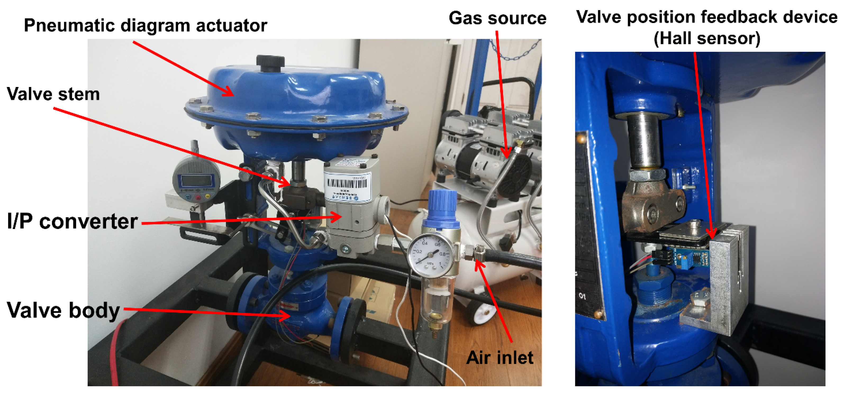
2.1. Experimental Equipment
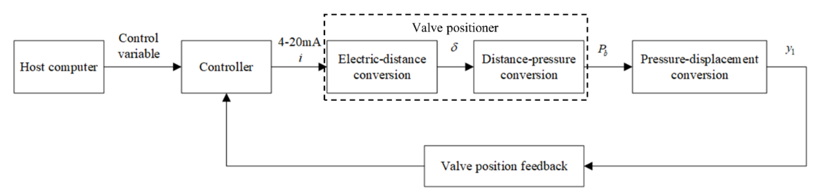
The commonly used pneumatic control valve system consists of three components, including valve positioner, pneumatic diaphragm actuator, and valve body; and the experimental platform is shown in Figure 2. Among them, the valve positioner is the key component of the pneumatic control valve system, which is responsible for the adjustment of the valve position [30,31]. It is mainly composed of the controller, nozzle-flapper-structure electric-pneumatic (I/P) converter and the valve position feedback device.
In the control process of a pneumatic control valve, the controller in the valve positioner outputs a current signal i (4–20 mA) according to the error between the setting value of the valve position and the actual value, which causes the distance between nozzle and flapper δ to change and then leads to the input air pressure of the pneumatic diaphragm actuator P b change. The air pressure P b acts on the diaphragm to form the driving force F p , which drives the valve stem to the specified position y 1 . The schematic diagram of the pneumatic control valve system is shown in Figure 3. The technical parameters of the pneumatic diaphragm actuator and I/P converter are shown in Table 1.
The input–output relationship of the system can reflect whether the pneumatic control valve system has backlash error. In order to analyze the cause of the backlash error and find the solution to this non-linear problem, the physical model of the pneumatic control valve system should be established. The physical model of the pneumatic control valve system consists of three parts, namely, the pneumatic diaphragm actuator model (achieve the conversion of P b to y 1 ), the nozzle-flapper structure model (achieve the conversion of δ to P b ), and the electromagnetic model (achieve the conversion of i to δ ). According to the physical model, the input ( i ) and output ( y 1 ) relationship of the pneumatic control valve system can be calculated.

2.2. Physical Model

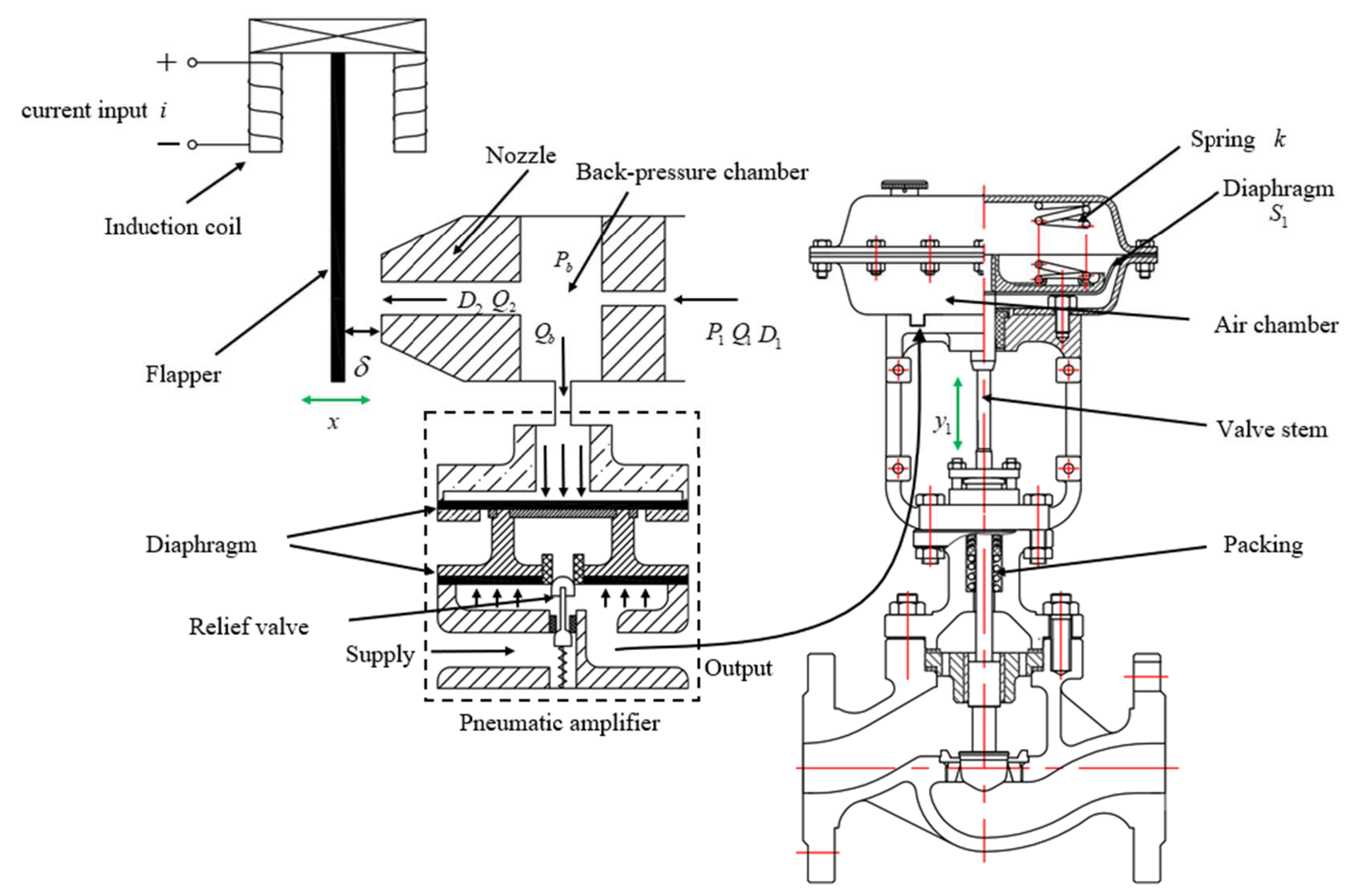
2.2.1. Pneumatic Diaphragm Actuator Model

The commonly used pneumatic diaphragm actuator is mainly composed of the diaphragm, spring, and valve stem. The mass of stem m is regarded as the mass of the pneumatic diaphragm actuator in this research. There is an interference fit between the valve stem and packing, so the friction arises when the valve stem moves, and friction acts on the system in the form of damping. Due to the existence of mass block (mass of stem m ), spring (elastic coefficient k ) and damping (damping coefficient c ), the pneumatic diaphragm actuator can be simplified to the m-c-k model. According to the model, the relationship between valve stem displacement y 1 and the input air pressure of the pneumatic diaphragm actuator P b can be calculated. The model diagram of the pneumatic diaphragm actuator is shown in Figure 4.
Based on Newton’s second law of motion, the motion equation of the valve stem is:
m y ¨ 1 = F p + F k + F f + F g + F i
F p = S 1 P b
F k = k y 1
where y 1 is the displacement of the valve stem; The driving force F p is generated by the input air pressure of the pneumatic diaphragm actuator P b , and the constant S 1 represents the area of the diaphragm; F k is the spring force. Both F g generated by the fluid movement in the valve body and F i required to obtain the valve stem plug into the seat are assumed to be zero because of their negligible contribution in the model according to the article [32]. F f is the friction between the valve stem and packing, the classical friction model is given in article [16].
v = y ˙ 1
F f = { F c s i g n ( v ) v f v i f v 0 ( F p + F k ) i f v = 0 a n d | F p + F k | F s F s s i g n ( F p + F k )   i f v = 0 a n d | F p + F k | > F s
where F c is the coulomb friction (also called the dynamic friction); f v is the viscous friction coefficient, and v f v represents the viscous friction; F s is the maximum static friction. Due to the discontinuity point ( v = 0 ) in the friction model, it is not conducive to analyze the established model. To deal with the issue, according to the article [14], a constant ε is introduced to create a very small zone as a mathematical expression of v = 0 , i.e., | v | < ε = 10 4 m / s equals v = 0 . Based on the (1)–(5), the continuous-time model of the pneumatic diaphragm actuator can be obtained:
m y ¨ 1 = { S 1 P b k y 1 F c y ˙ 1 f v i f y ˙ 1 ε 0 i f | y ˙ 1 | < ε a n d | F p + F k | F s S 1 P b k y 1 F s   i f | y ˙ 1 | < ε a n d ( F p + F k ) > F s S 1 P b k y 1 + F s i f | y ˙ 1 | < ε a n d ( F p + F k ) < F s S 1 P b k y 1 + F c y ˙ 1 f v i f y ˙ 1 ε
The external force of the valve stem is zero when the valve stem is stable, and the sum of F p and F k is less than F s . Changing the direction of stem movement, F p increases (decreases), but the valve stem remains stable due to the existence of static friction. The input current continues to increase (decrease) until the sum of F p and F k is more (less) than F s ( F s ), the acceleration of the valve stem becomes non-zero and starts to move. The valve stem needs to overcome the effect of friction when changing the direction of stem movement, that is, the input current within a certain threshold changes, and the valve stem does not move.

2.2.2. Nozzle-Flapper Structure Model

In order to calculate y 1 , the input air pressure of the pneumatic diaphragm actuator P b should be calculated firstly, which is determined by the distance between the flap and nozzle δ . To calculate the relationship between P b and δ , the structure of the nozzle-flapper should be analyzed. The nozzle-flapper-structure I/P converter is similar to a solenoid valve, which is composed of an induction coil, the nozzle-flapper structure, and a pneumatic amplifier. The stable gas source enters the back-pressure chamber after being throttled and stabilized by the constant orifice, if δ changes, P b changes. The nozzle-flapper structure is shown in Figure 3.
Gas flow in the nozzle-flapper structure satisfies the flow continuum equation:
Q 1 = Q 2 + Q b
where Q 1 is the inflow of the back-pressure chamber; Q 2 is the outflow of the nozzle; Q b is the flow from the back-pressure chamber into the pneumatic amplifier.
Both the orifice and nozzle belong to the thin-walled hole, the flow equations of the fluid flowing through the thin-walled holes are:
Q 1 = C q 1 A 1 2 ρ Δ P 1
Q 2 = C q 2 A 2 2 ρ Δ P 2
A 1 = π 4 D 1 2
A 2 = π D 2 δ
δ = δ max x
Δ P 1 = P 1 P b
Δ P 2 = P b
where C q is the flow coefficient of the small hole and it is a constant; A 1 is the area of the orifice; ρ is the density of the fluid; A 2 is the area of gas passage at nozzle; P 1 is the input gas pressure; Δ P 1 is the differential pressure between the back-pressure chamber and input gas; Δ P 2 is the differential pressure between back-pressure chamber and atmosphere; δ max is the distance between the nozzle and the flapper when the I/P converter is not working; x is the displacement of the flapper.
According to (7)–(14),
Q b = π C q 1 D 1 2 4 2 ρ ( P 1 P b ) π C q 2 D 2 δ 2 ρ P b
The back-pressure chamber is connected to the pneumatic amplifier, and when the system is stable, the pressure of the pneumatic amplifier is equal to the pressure of the back-pressure chamber. In this case, the flow from the back-pressure chamber into the pneumatic amplifier ( Q b ) equals 0. Based on it, the function P b can be obtained, which is related to δ .
P b = C q 1 2 D 1 4 P 1 16 C q 2 2 D 2 2 δ 2 + C q 1 2 D 1 4
Formula (16) is the function relationship between the output air pressure of the back-pressure chamber P b and the nozzle baffle gap δ . The analysis of it shows that:
(1)
When δ = 0 , P b = P 1 , that is, when the distance between the nozzle and the baffle is 0, the output air pressure of the back-pressure chamber is equal to the input air pressure of the nozzle baffle mechanism;
(2)
When δ gradually increases, P b approaches 0, that is, the output pressure of the back-pressure chamber is almost equal to the atmospheric pressure. According to the mechanism analysis of the nozzle baffle mechanism, the nozzle is equivalent to variable air resistance, which is connected in series with the constant air resistance corresponding to the constant orifice. As the gap increases, the variable air resistance value decreases. According to the principle of partial pressure, the constant air resistance partial pressure Δ P 1 (formula (13)) in the gas path increases, and the variable air resistance partial pressure Δ P 2 (formula (14)) decreases, and finally Δ P 2 approaches zero, that is, P b approaches zero. The mechanism analysis result of the nozzle baffle mechanism is consistent with the numerical analysis result of formula (16). Based on the above analysis, the derivation of formula (16) is correct.

2.2.3. Electromagnetic Model

There is an induction coil in the I/P converter, based on the principle of electromagnetic effects, the change of the input current i causes the magnetic force generated by the coil to change, which causes the movement of the flapper, and finally leads to the change of δ . To obtain the relationship between δ and i , the electromagnetic model generated by the induction coil in the nozzle-flapper-structure I/P converter should be established.
The dynamic process of the nozzle-flapper-structure I/P converter follows the voltage balance equation on the circuit:
U = i R s + d ψ d t
ψ = N ϕ
where U is the voltage of the coil and it is a fixed value; R s is the coil resistance; ψ is the coil flux; N is the number of coil turns; ϕ is the coil magnetic flux, which is a variable about i and x .
U = i R s + N ( ϕ i d i d t + ϕ x d x d t )
d i d t = i R s ϕ i N + U ϕ i N ϕ x ϕ i d x d t
Equation (20) is the differential equation about i and x . According to Kirchhoff’s magnetic pressure law, the magnetic circuit equation ignoring armature and non-operating air gap magnetoresistance is as follows.
i N = ϕ δ R + H m L m
R = 2 x / μ 0 S
ϕ δ = σ ϕ
B = ϕ / S = μ 0 H m
where R is the gap magnetoresistance; ϕ δ is the magnetic flux at the gap; H m is the magnetic field intensity; L m is the length of the magnetic circuit; S is the magnetic area; σ is the magnetic leakage coefficient at air gap. According to (18) and (21)–(24),
ϕ = i N μ 0 S L m + 2 σ x
according to (20) and (25), the relationship between i and x can be obtained.
ϕ i = N μ 0 S L m + 2 σ x
ϕ x = 2 σ N μ 0 S i ( L m + 2 σ x ) 2
d i d t = L m U N 2 μ 0 S + 2 σ U N 2 μ 0 S x L m R s N 2 μ 0 S i 2 σ R s N 2 μ 0 S x i 2 σ i L m + 2 σ x d x d t
The coil resistance is small and can be ignored, (28) can be simplified as:
d i d t = a + b x s i j + s x d x d t
where a = L m U N 2 μ 0 S , b = 2 σ U N 2 μ 0 S , j = L m , s = 2 σ . Divide both sides of (29) by b ,
1 b d i d t = a b + x 1 b i j s + x d x d t = X 1 b i X d X d t
a b = j s = L m 2 σ , a b + x = j s + x , which can be substituted by X . On this basis, the differential equation (30) can be solved. In order to calculate the functional relationship between i and x , it is assumed that i = e t v , X = n t v 1 ( e ,   n 0 , v 0 , 1 ). e , n , v are all fixed values, which are determined by the structure of the induction coil. The functional relationship between i and δ is:
δ = δ max + L m 2 σ ( ( 2 v 1 ) n 1 v 1 b i ) v 1 v

2.2.4. Model Integration

The relationship between y 1 and i can be obtained according to three physical models established above, that is, the input–output relationship of the control system of the pneumatic control valve can be obtained.
Substituting (31) into (16), the function relationship between the input air pressure of the pneumatic diaphragm actuator P b and input current i can be obtained:
P b = C q 1 2 D 1 4 P 1 16 C q 2 2 D 2 2 ( δ max + L m 2 σ ( ( 2 v 1 ) n 1 v 1 b i ) v 1 v ) 2 + C q 1 2 D 1 4
Substituting (32) into (6), the relationship between the input current i and the valve stem displacement y 1 can be obtained.
m y ¨ 1 = { S 1 C ( D E i v 1 v ) 2 + F F c k y 1 y ˙ 1 f v y ˙ 1 ε 0 | y ˙ 1 | < ε S 1 C ( D E i v 1 v ) 2 + F + F c k y 1 y ˙ 1 f v y ˙ 1 ε
where C = C q 1 2 D 1 4 P 1 , D = 4 C q 2 D 2 ( δ max + L m 2 σ ) , E = 4 C q 2 D 2 ( ( 2 v 1 ) n 1 v 1 b ) v 1 v , F = C q 1 2 D 1 4 . Among them, C , D and F are all fixed values, E is determined by n and v . When the coil structure is determined, n and v are all constants.
Based on (33), the displacement of the valve stem y 1 can be calculated when different currents i are loaded, that is, the input ( i )–output ( y 1 ) relationship of the pneumatic control valve system can be obtained. When i is fixed, (33) is the second-order differential equation of t . The Runge–Kuta method can be used to calculate the numerical result of the differential equation. The parameters of the commonly used pneumatic control valve system are shown in Table 2. The first group of the parameters ( m to F c ) in Table 2 come from reference [18], and the rest of the parameters are obtained by consulting the relevant technical personnel. Since E is determined by n and v , v = 2 , n = 1 and v = 2 , n = 2 are chosen for calculation in this research. Current-displacement calculation results of the physical model are shown in Figure 5 and Figure 6.
Take v = 2 and n = 1 as an example for the differential Equation (33) solution description. Since the (33) is a piecewise function, it needs to be discussed in four states.
State 1: The direction of input current is not changed, increasing the input current. In this state, different current values can be substituted into the (33) to solve the differential equation when y ˙ 1 ε . For example, when the current starts from 6mA and increases every 0.5 mA to 20 mA, the relationship between i and y 1 is shown by curve 1 in Figure 5. It is shown that i and y 1 have a linear relationship.
State 2: Change the current input direction (decrease). Once the current direction changes, the velocity of valve stem becomes 0, and the valve stem movement state meets the differential equation under the condition of y ˙ 1 < ε in (33). Analyze the valve stem displacement value under the State 1, and the displacement of the valve stem at this time is 0.263. Therefore, the initial conditions of the differential equation are: y ( 0 ) = 0.263 ,   y ˙ ( 0 ) = 0 . As shown by curve 2 in Figure 5, y 1 keeps constant, while i is changing, so that a horizontal path is obtained. After the current is reduced by a certain threshold, when F p + F k < F s , the valve stem starts to move and turns to State 3 for analysis.
State 3: The direction of input current is not changed, reducing the current input. In this state, different current values can be substituted into the (33) to solve the differential equation when y ˙ 1 ε . For example, when i starts from 20mA and decreases every 0.5mA to 7mA, the relationship between i and y 1 is shown by curve 3 in Figure 5, and the relationship between i and y 1 is linear.
State 4: Change the current input direction (increase). When the current input direction is changed, the valve stem velocity becomes 0, and the valve stem movement state meets the differential equation under the condition of y ˙ 1 ε in the (33). Analyze the valve stem displacement under State 3, the displacement of the valve stem is 0.2131. Therefore, the initial conditions of the differential equation are: y ( 0 ) = 0.2131 ,   y ˙ ( 0 ) = 0 . As shown by curve 4 in Figure 5, y 1 keeps constant, while i is changing, so that a horizontal path is obtained. After the current increases by a certain threshold, when F p + F k > F s , the valve stem starts to move and turns to State 1 for analysis.
In order to verify the correctness of the proposed physical model, an experiment was conducted, in which different input currents i were loaded and valve stem displacement y 1 was recorded. The experimental equipment is shown in Figure 1. The experimental result is shown in Figure 7.
According to the experimental result and the calculation results of the physical model established above, the control system of the pneumatic control valve is non-linear. As shown in Figure 5, Figure 6 and Figure 7, if the valve stem rises firstly and then falls, the displacement of the valve stem undergoes a “rising-horizontal-falling” state change. The appearance of a “horizontal” state is caused by friction, which causes backlash error in the system and makes the system appear non-linear.
Comparing Figure 5, Figure 6 and Figure 7, it is shown that the vertical axes of three figures all represent the displacement of the valve stem, the values are different, but the changing trends of the displacement are consistent. The focus of model calculation is not the specific displacement value, but the change trend of the displacement value y 1 with the current i to reveal the manifestation of the backlash error. The difference in value are caused by the difference between the physical model parameters and the experimental parameters. In addition, when the direction of movement of the valve stem is not changed, y 1 and i are linear in Figure 5 and Figure 7, while y 1 and i are nonlinear in Figure 6, which is caused by the difference in the combination of v and n in two cases. n and v are determined by the structure of the induction coil, therefore the physical model established under v = 2 and n = 1 is similar to the actual experimental equipment.

3. Control Method

It is proved that the backlash error exists in the pneumatic control valve system. In this sense, the whole control system appears non-linear and the oscillation of the valve stem is prone to occur during the control process. The PID algorithm is used in the control system commonly and achieves a good control effect. However, only using the PID algorithm cannot deal with the backlash error entirely in the pneumatic control valve system, and the oscillation of the valve stem still exists. The PID algorithm is as follows:
u ( k ) = K P e ( k ) + K I j = 0 k e ( j ) + K D [ e ( k ) e ( k 1 ) ]
K P , K I and K D represent proportional coefficient, integral coefficient and derivative coefficient respectively; e ( k ) represents the deviation between the set value and the actual value.
Based on the physical model established above, there is a certain non-linear relationship between the input current and the displacement of the valve stem. According to Figure 7, when the direction of the input current signal is changed, the movement direction of the valve stem is unchanged. Therefore, I t h r e s h o l d can be introduced, which refers to the value of current change that drives the movement of the valve stem under the condition that the direction of the current changes. Its main function is to overcome the influence of backlash. Based on it, the value of the input current signal i S C can be obtained, which is related to I t h r e s h o l d .That is, when the current increases in the positive direction, I t h r e s h o l d is added to the current i , that is, i S C = i + I t h r e s h o l d . And when the current decreases in the reverse direction, I t h r e s h o l d is subtracted, that is, i S C = i I t h r e s h o l d . This method requires pre-calibration before valve control, which is called the self-calibration (SC) control method. The SC control method performed before the valve control, CPU records the current value and the corresponding valve stem displacement value automatically, calculates I t h r e s h o l d , and uses this value in subsequent control finally. The steps for SC control are as follows:
Step 1: Carry out three forward current loads in sequence and record the corresponding valve displacement respectively, which are ( I 1 , A 1 ) , ( I 2 , A 2 ) , ( I 3 , A 3 ) ;
Step 2: Carry out three reverse current loads in sequence and record the corresponding valve displacement respectively, which are ( I 4 , B 1 ) , ( I 5 , B 2 ) , ( I 6 , B 3 ) ;
Step 3: The valve stem displacement is linearly fitted to calculate the slope k 1 and intercept b 1 of the curve when the current signal is loaded forward. The slope k 2 and intercept b 2 can also be calculated by fitting the curve of the displacement and the reverse loading current signal. It is found that k 1 is almost the same with k 2 , so take the mean of k 1 and k 2 as the slope of the curve k . The current threshold I t h r e s h o l d caused by the backlash error can be calculated. The schematic diagram of self-calibration control method is shown in Figure 8.
k 1 = ( A 2 A 1 I 2 I 1 + A 3 A 2 I 3 I 2 ) / 2
k 2 = ( B 2 B 1 I 5 I 4 + B 3 B 2 I 6 I 5 ) / 2
k = ( k 1 + k 2 ) / 2
b 1 = [ ( A 1 k I 1 ) + ( A 2 k I 2 ) + ( A 3 k I 3 ) ] / 3
b 2 = [ ( B 1 k I 4 ) + ( B 2 k I 5 ) + ( B 3 k I 6 ) ] / 3
I t h r e s h o l d = ( b 2 b 1 ) / k
However, the output current signal is calculated by the self-calibration control method, so using the calculated current i S C as the control current signal may result in a fixed deviation from the setting value of the valve position. Therefore, only using the self-calibration control method may result in the fixed deviation between the setting value and the actual value.
To deal with the backlash error, a self-calibration PID (SC-PID) algorithm is proposed, which combines the PID algorithm and the self-calibration algorithm. The SC-PID algorithm reduces the response time with self-calibration control and eliminates the fixed deviation caused by the self-calibration control with PID control. Adding the current output i S C obtained by the self-calibration algorithm with the current output calculated by the PID algorithm as the output signal of the SC-PID algorithm. i S C is the current output obtained by the self-calibration algorithm, and its main function is to overcome the influence of backlash error. During the control process of a pneumatic control valve, the control quantity needs to be constantly changed. Due to the influence of backlash, within a certain threshold, changing the current cannot make the valve stem move, and the error continues to accumulate, which leads to a sudden change in the control quantity, eventually resulting in overshoot during the control process. In severe cases, the valve stem oscillation is aggravated. By introducing i , the influence of the backlash can be overcome, the control speed can be improved, and the valve stem oscillation can be reduced. The SC-PID algorithm is:
u ( k ) = K P e ( k ) + K I j = 0 k e ( j ) + K D [ e ( k ) e ( k 1 ) ] + i S C

4. Valve Position Control Experiment

In order to prove the effectiveness of the SC-PID algorithm in dealing with the backlash error, the PID algorithm, self-calibration algorithm, and SC-PID algorithm are applied to the valve position control experiment respectively. According to the control effects of different control algorithms, the SC-PID algorithm can handle the backlash error that existed in the valve position control.
The control effect with three control methods is shown in Figure 9. The valve stem oscillates violently during the control. The reasons for PID algorithm cannot realize valve stem stability control are as follows: When the actual valve position is not equal to the setting value, the PID controller will change the input current i . If the change in input current is less than the current threshold, the valve stem cannot move due to the existence of backlash error. Once the change in input current is greater than the current threshold, the valve stem moves. Because the change in input current needs to exceed the current threshold, the valve stem moves a lot and exceeds the setting value, so that the error between the setting value and the actual value still exists, and the oscillation of the valve stem does not stop.
Self-calibration control is similar to the pre-processing of valve position control. According to the relationship between the input current i and valve stem displacement y 1 obtained before valve position control, the current control signal can be calculated. This algorithm decreases the calculation requirement of the controller and increases the control speed. However, error exists in linear fitting of valve stem displacement-input current, which causes a fixed deviation between the actual value and the setting value. Since the self-calibration algorithm is a form of open-loop control, the fixed displacement cannot be eliminated by it.
The valve position control effect with the SC-PID algorithm is shown in Figure 9. This method uses a self-calibration algorithm to increase the control speed and uses the PID algorithm to eliminate the fixed deviation caused by the self-calibration algorithm. Because the fixed deviation is small, there is a little oscillation of valve stem due to backlash error during control. Using the SC-PID algorithm for valve position control can make the position control faster and more accurate as a means to solve the backlash error.

5. Conclusions

(1)
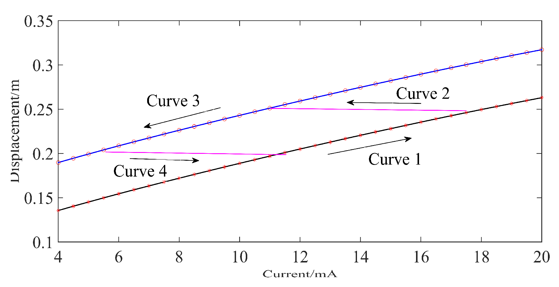
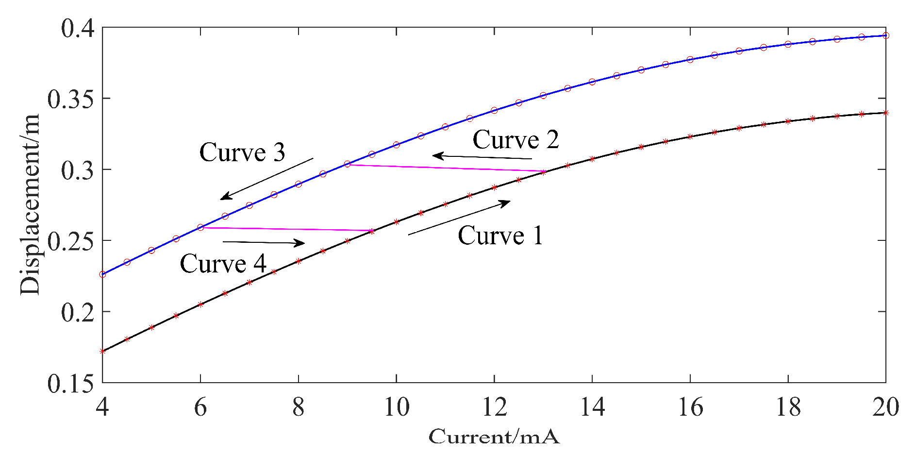
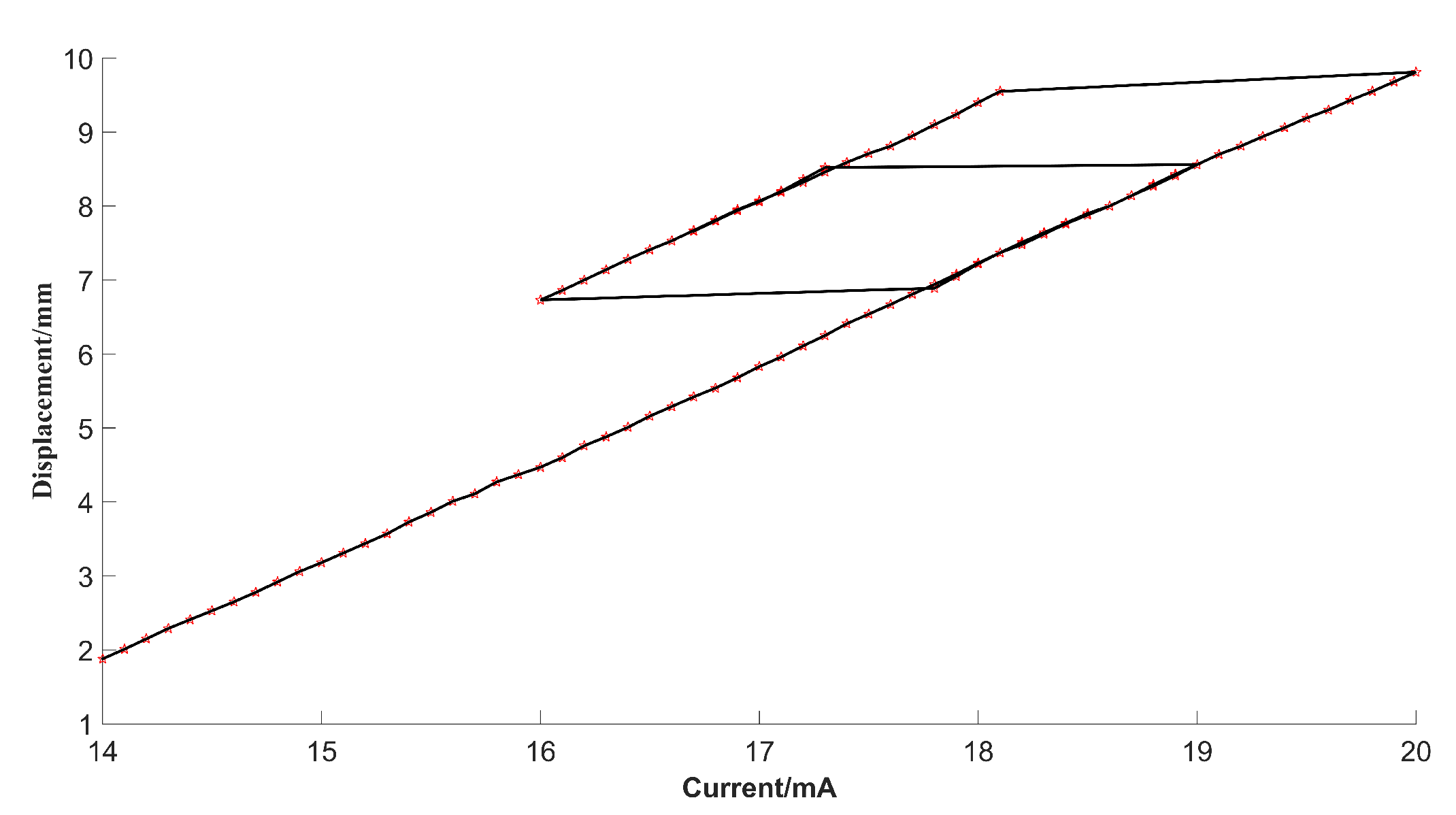
The physical model of the commonly used pneumatic control valve is established in this paper, including the pneumatic diaphragm actuator model, nozzle-flapper structure model, and electromagnetic model. It is shown that the backlash error existing in the pneumatic control valve is related to the friction according to the physical model. In addition, the relationship between the input current i and valve stem displacement y 1 can be calculated based on the physical model, and the experimental result is consistent with the model calculation results, which shows that the established physical model is correct.
(2)
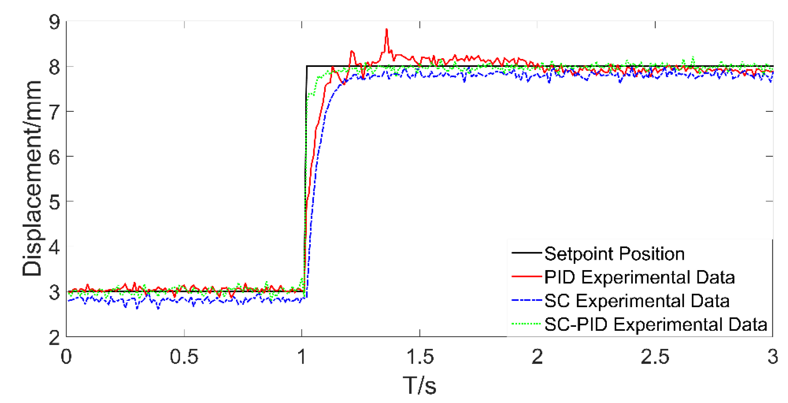
To deal with the valve stem oscillation caused by the backlash error during valve control, the SC-PID control method is proposed. Compared with other algorithms, the proposed algorithm is simpler, valve position control faster, and control effect better.
(3)
During the control of the pneumatic control valve, the disturbance caused by the flow of medium in the pipeline is inevitable and cannot be ignored. The dynamic characteristics of the control system under load disturbance will be analyzed in future work.

Author Contributions

Conceptualization, L.Z. and H.X.; methodology, Y.L. and H.X.; software, H.X.; validation, Y.L. and L.Z.; data curation, Y.L. and H.X.; writing—original draft preparation, H.X.; writing—review and editing, Y.L. and L.Z.; funding acquisition, L.Z. All authors have read and agreed to the published version of the manuscript.

Funding

This work was supported by the National Key Research and Development Program of China (Grant No. 2018YFC0808600) and National Natural Science Foundation of China (Grant No. 51975213).

Institutional Review Board Statement

Not applicable.

Informed Consent Statement

Not applicable.

Data Availability Statement

The data presented in this study are available on request from the corresponding author.

Conflicts of Interest

The authors declare no conflict of interest.

References

  1. Qiu, C.; Jiang, C.-H.; Zhang, H.; Wu, J.-Y.; Jin, Z.-J. Pressure Drop and Cavitation Analysis on Sleeve Regulating Valve. Processes 2019, 7, 829. [Google Scholar] [CrossRef] [Green Version]
  2. Ale Mohammad, M.; Huang, B. Compensation of control valve stiction through controller tuning. J. Process Control 2012, 22, 1800–1819. [Google Scholar] [CrossRef]
  3. Riccardo, B.D.C.; Vaccari, M.; Pannocchia, G. Model predictive control design for multivariable processes in the presence of valve stiction. J. Process Control 2018, 71, 25–34. [Google Scholar]
  4. Di Capaci, R.B.; Scali, C. Review and comparison of techniques of analysis of valve stiction: From modeling to smart diagnosis. Chem. Eng. Res. Des. 2018, 130, 230–265. [Google Scholar] [CrossRef]
  5. Choudhury, M.S.; Thornhill, N.F.; Shah, S.L. Modelling valve stiction. Control Eng. Pract. 2005, 13, 641–658. [Google Scholar] [CrossRef] [Green Version]
  6. Hidalgo, M.C.; Garcia, C. Friction compensation in control valves: Nonlinear control and usual approaches. Control Eng. Pract. 2017, 58, 42–53. [Google Scholar] [CrossRef]
  7. Armstrong-Hélouvry, B.; Dupont, P.; De Wit, C.C. A survey of models, analysis tools and compensation methods for the control of machines with friction—ScienceDirect. Automatica 1994, 30, 1083–1138. [Google Scholar] [CrossRef]
  8. Pennestrì, E.; Rossi, V.; Salvini, P.; Valentini, P.P. Review and comparison of dry friction force models. Nonlinear Dyn. 2016, 83, 1785–1801. [Google Scholar] [CrossRef]
  9. Carneiro, J.F.; de Almeida, F.G. LuGre Friction Model: Application to a Pneumatic Actuated System. Lect. Notes Electr. Eng. 2015, 321, 459–468. [Google Scholar]
  10. Meng, D.; Tao, G.; Liu, H.; Zhu, X. Adaptive robust motion trajectory tracking control of pneumatic cylinders with LuGre model-based friction compensation. Chin. J. Mech. Eng. 2014, 27, 802–815. [Google Scholar] [CrossRef]
  11. Carducci, G.; Giannoccaro, N.I.; Messina, A.; Rollo, G. Identification of viscous friction coefficients for a pneumatic system model using optimization methods. Math. Comput. Simul. 2006, 71, 385–394. [Google Scholar] [CrossRef]
  12. Li, X.; Chen, S.L.; Teo, C.S.; Tan, K.K.; Lee, T.H. Data-Driven Modeling of Control Valve Stiction Using Revised Binary-Tree Structure. Ind. Eng. Chem. Res. 2015, 54, 330–337. [Google Scholar] [CrossRef]
  13. Wang, G.; Wang, J. Quantification of valve stiction for control loop performance assessment. In Proceedings of the 16th International Conference on Industrial Engineering and Engineering Management, Beijing, China, 21–23 October 2009. [Google Scholar]
  14. Choudhury, M.S.; Thornhill, N.F.; Shah, S.L. A Data-Driven Model for Valve Stiction. IFAC Proc. Vol. 2004, 37, 245–250. [Google Scholar] [CrossRef] [Green Version]
  15. He, Q.P.; Wang, J.; Pottmann, M.; Qin, S.J. A Curve Fitting Method for Detecting Valve Stiction in Oscillating Control Loops. Ind. Eng. Chem. Res. 2007, 46, 4549–4560. [Google Scholar] [CrossRef]
  16. Fang, L.; Tang, L.; Wang, J.; Shang, Q. A semi-physical model for pneumatic control valves. Nonlinear Dyn. 2016, 85, 1–14. [Google Scholar] [CrossRef]
  17. Tang, L.; Fang, L.; Wang, J.; Shang, Q. Modeling and Identification for Pneumatic Control Valves with Stiction. IFAC Pap. 2015, 48, 1244–1249. [Google Scholar] [CrossRef]
  18. He, Q.P.; Wang, J. Valve Stiction Quantification Method Based on a Semiphysical Valve Stiction Model. Ind. Eng. Chem. Res. 2014, 53, 12010–12022. [Google Scholar] [CrossRef]
  19. Han, K.H.; Koh, G.O.; Sung, J.M.; Kim, B.S. An Adaptive Control Approach for Improving Control Systems with Unknown Backlash. Int. J. Aeronaut. Space Sci. 2011, 12, 360–364. [Google Scholar] [CrossRef]
  20. Voeroes, J. Identification of cascade systems with backlash. Int. J. Control 2010, 83, 1117–1124. [Google Scholar] [CrossRef]
  21. Voeroes, J. Identification of nonlinear dynamic systems with input saturation and output backlash using three-block cascade models. J. Frankl. Inst. 2014, 351, 5455–5466. [Google Scholar] [CrossRef]
  22. Voeroes, J. Modeling and Identification of Nonlinear Cascade and Sandwich Systems with General Backlash. J. Electr. Eng. 2014, 65, 104–110. [Google Scholar]
  23. Zhou, J.; Wen, C.; Zhang, C.; Shen, X. Adaptive Output Control of Uncertain Nonlinear Systems with Unknown Backlash. In Proceedings of the American Control Conference (ACC), New York, NY, USA, 9–13 July 2007. [Google Scholar]
  24. Tao, G.; Kokotovic, P.V. Adaptive control of systems with backlash. Automatica 1993, 29, 323–335. [Google Scholar] [CrossRef]
  25. Mazenc, F.; Andrieu, V.; Malisoff, M. Design of continuous–discrete observers for time-varying nonlinear systems. Automatica 2015, 57, 135–144. [Google Scholar] [CrossRef] [Green Version]
  26. Zhou, J.; Zhang, C.; Wen, C. Robust Adaptive Output Control of Uncertain Nonlinear Plants With Unknown Backlash Nonlinearity. IEEE Trans. Autom. Control 2007, 52, 503–509. [Google Scholar] [CrossRef]
  27. Li, X.; Yao, J.; Zhou, C. Adaptive Robust Control for Backlash Nonlinearity with Extended State Observer. In Proceedings of the 35th Chinese Control Conference, Chengdu, China, 27–29 July 2016; pp. 4579–4584. [Google Scholar]
  28. Zhang, D.X.; Jia, J.Y.; Guo, Y.X. Neural Network Sliding Mode Control Approach to Backlash and Friction Compensation. J. Univ. Electron. Sci. Technol. China 2018, 37, 793–796. [Google Scholar]
  29. Lyu, Z.; Liu, Z.; Xie, K.; Chen, C.P.; Zhang, Y. Adaptive Tracking Control for Switched Nonlinear Systems with Fuzzy Actuator Backlash. Fuzzy Sets Syst. 2020, 385, 60–80. [Google Scholar] [CrossRef]
  30. Di Capaci, R.B.; Scali, C.; Pestonesi, D.; Bartaloni, E. Advanced Diagnosis of Control Loops: Experimentation on Pilot Plant and Validation on Industrial Scale. IFAC Proc. Vol. 2013, 46, 589–594. [Google Scholar] [CrossRef] [Green Version]
  31. Cheng, Q.; Liu, Z.; Jiang, A.; Jiang, E.; Xiao, Y.; Li, F.; Jiang, J. Research on control algorithm of intelligent valve positioner based on parameter self-tuning. In Proceedings of the 39th Chinese Control Conference (CCC), Shenyang, China, 27–29 July 2020. [Google Scholar]
  32. Kayihan, A.; Doyle, F.J. Friction compensation for a process control valve. Control Eng. Pract. 2000, 8, 799–812. [Google Scholar] [CrossRef]
Figure 1. Conversion diagram in the control loop of the pneumatic control valve.
Processes 09 01378 g001
Figure 2. The experimental platform of the pneumatic control valve.
Processes 09 01378 g002
Figure 3. Schematic diagram of the pneumatic control valve system.
Processes 09 01378 g003
Figure 4. Model diagram of the pneumatic diaphragm actuator.
Processes 09 01378 g004
Figure 5. Current-displacement result of physical model ( v = 2 ,   n = 1 ).
Processes 09 01378 g005
Figure 6. Current-displacement results of physical model ( v = 2 ,   n = 2 ).
Processes 09 01378 g006
Figure 7. Experimental current-displacement diagram.
Processes 09 01378 g007
Figure 8. The schematic diagram of self-calibration control method.
Processes 09 01378 g008
Figure 9. Comparison of valve position control effects of three control algorithms.
Processes 09 01378 g009
Table 1. Technical parameters of pneumatic diaphragm actuator and electric–pneumatic (I/P) converter.
Pneumatic Diaphragm Actuator
(ZJHP-16C)
Nominal pressure/MPa1.6
Signal pressure/MPa0.08–0.24
Flow characteristicsEqual percentage
I/P Converter
(T-1000 961-075-000)
Input signal /mA4–20
Maximum supply pressure/MPa0.7
Pressure output/MPa0.04–0.21
Table 2. Parameters of commonly used pneumatic control valve system.
ParameterValue/Unit
Mass of stem m 1.36 kg
Spring constant k 5.25 × 10 4 kg / s 2
Diaphragm area S 1 6.45 × 10 2 m 2
Input gas pressure P 1 3 × 10 5 Pa
Viscous friction coefficient f v 1.59 kg / s
Coulomb friction F c 1423 N
Magnetic path length L m 0.4 m
Maximum gap of nozzle baffle δ max 3 × 10 4 m
Orifice flow coefficient C q 1 0.75
Nozzle flow coefficient C q 2 0.7
Supply voltage U 12 V
Orifice diameter D 1 4.3 × 10 4 m
Nozzle diameter D 2 1.6 × 10 3 m
Coil turns N 24,000
Magnetic flux leakage coefficient σ 4.2
Magnetic area S 1.995 × 10 3 m 2
Publisher’s Note: MDPI stays neutral with regard to jurisdictional claims in published maps and institutional affiliations.

