1. Introduction
On rainy or cloudy days, solar radiation is under 150 W/m
2 and the solar power generation (SPG) system output power is low [
1]. The SPG system output energy is dependent on climatic elements (e.g., solar radiation and ambient temperature). Therefore, the maximum power point tracking (MPPT) controller can greatly improve the efficiency of the SPG system [
2,
3].
Numerous MPPT algorithms are available for the SPG system and have been extensively investigated [
4,
5,
6,
7,
8,
9,
10,
11,
12,
13,
14,
15,
16,
17,
18,
19,
20,
21,
22,
23]. The hill-climbing (HC) algorithm architecture is simple in that only two power points are compared and then MPPT is executed [
4]. Meanwhile, the perturbation and observation (P&O) algorithm compares the relationship between voltage and power slope and then searches for the maximum power point (MPP) [
5]. The incremental conductance (INC) method implements MPPT based on the relationship between the incremental conductance (dI/dV) and the conductance (I/V) [
6]. The fuzzy logic algorithm is a computer-intelligent control based on fuzzy variables and fuzzy logic inferences [
7]. The neural network algorithm is a mathematical model that imitates the structure and function of biological neural networks [
8]. Further, the particle swarm optimization (PSO) algorithm is based on imitating the behavior of bird flocks and discovering the advantages of evolution in bird flocks [
9]. The artificial bee colony (ABB) algorithm was developed by the bee foraging method [
10] while the intelligent monkey king evolution (IMKE) is a control strategy developed based on the super ability of the Chinese novel Monkey King [
11]. The flower pollination (FP) method is an algorithm for pollen transfer in nature [
12] and grey wolf optimization (GWO) is an algorithm inspired by the behavior of gray wolves [
13]. The data-driven MPPT method in PV systems is based on voltage and power and searches for the MPP [
14] while the state-plane direct MPPT algorithm is the large-signal and state-plane model of the converter developed [
15]. The leaky least logarithmic absolute difference-based control algorithm and the learning-based INC MPPT algorithm improve INC method problems such as steady-state oscillations and slow dynamic responses [
16] and evaluate the characteristics of the HC algorithm and INC method to discover the applicable area [
17]. The purpose of the proposed strategy is to combine the P&O algorithm and the fireworks algorithm (FWA), which can track the MPP in partial shading conditions (PSCs) [
18]. The new fuzzy logic control (FLC) technology developed based on the HC algorithm [
19] discusses the different MPPT technologies and analyzes the applied conditions. As a research reference [
20], the research introduces the adaptively binary weighted steps followed by the monotonically decreased step. In addition, as an MPPT technique [
21], it studies the turbulent flow of water-based optimization (TFWO) to analyze the characteristics of SPV modules [
22]. Furthermore, the research proposes the pigeon-inspired optimization (PIO) algorithm, a new type of metaheuristic algorithm, which implements MPPT under PSCs [
23].
The P&O algorithm, whose structure is simple and low-cost, is the most frequently used [
17]. However, it has four disadvantages: (1) while it cannot track the MPP under partial shading, this algorithm could converge to the local peak power point (LPPP) and cause a lower system performance [
18]; (2) with the P&O algorithm’s actuating point close to the maximum power point (MPP), it converges slowly [
19]; (3) this algorithm’s actuating point oscillates near the MPP when solar radiation is steady, causing low system efficiency [
19,
20]; (4) the P&O algorithm is prone to divergence when solar radiation varies quickly [
20,
21].
The present study proposes a new control scheme for the SPG system where the solar radiation value detection scheme is the SPV module equivalent conductance (Rspv−1) threshold control (CTC) implemented in the MPPT control scheme, combined with the P&O algorithm. The experimental comparison is of the proposed algorithm and the P&O algorithm under varying solar radiation and partial shading conditions. Moreover, the proposed algorithm efficiency is higher than the P&O algorithm, which could operate at the MPP and avoid being trapped in the LPPP under PSCs.
3. Proposed Algorithm
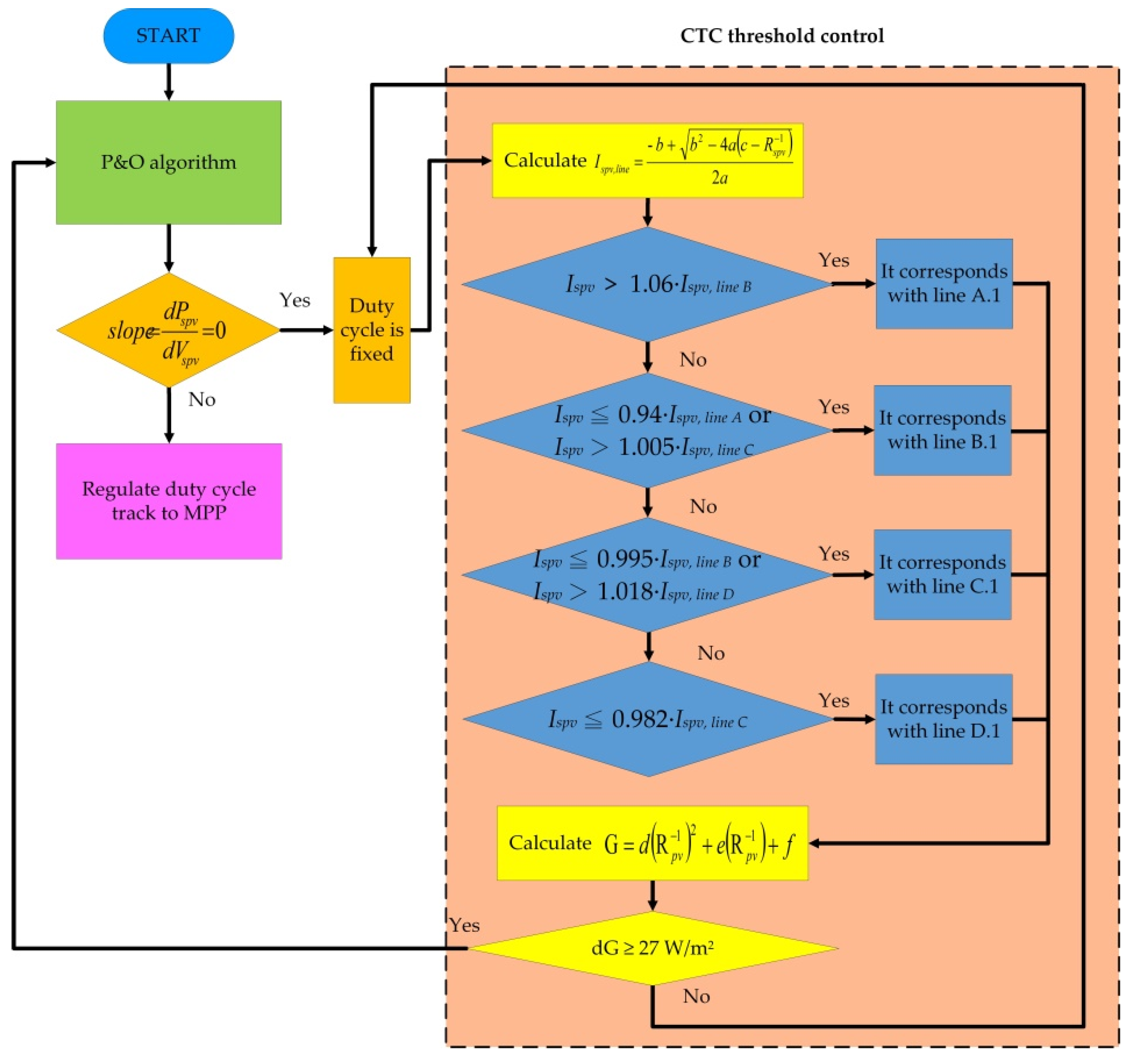
When solar radiation varies rapidly, the traditional P&O algorithm’s actuating point is continuously perturbed and does not immediately catch the MPP, thereby causing low system efficiency. In order to solve this problem, the proposed CTC is integrated with the P&O algorithm. This proposed algorithm can estimate the actual solar radiation value and execute the MPPT, improving the system efficiency.
Moreover, solar radiation is stable as in Equation (1). This proposed algorithm is to keep a constant duty cycle and improve the perturbation problem. Notably, this greatly improves the MPPT efficiency of the P&O algorithm.
The proposed algorithm first executes the MPPT to track the MPP where the
slope is 0, which will then be entered in the CTC mode. The illustration of the proposed algorithm control principle is as follows: (1)
Figure 1 illustrates the
Ispv-
Vspv characteristic curves of the SPV module, which has been informed. When solar radiation G and temperature T change, so do the SPV module output voltage
Vspv and the current
Ispv (2). The important parameter,
Rspv, of Equation (2) changes based on G and T. Thus,
Rspv can reflect G and T changes and
Rspv of the SPV module is an important reference factor for the CTC.
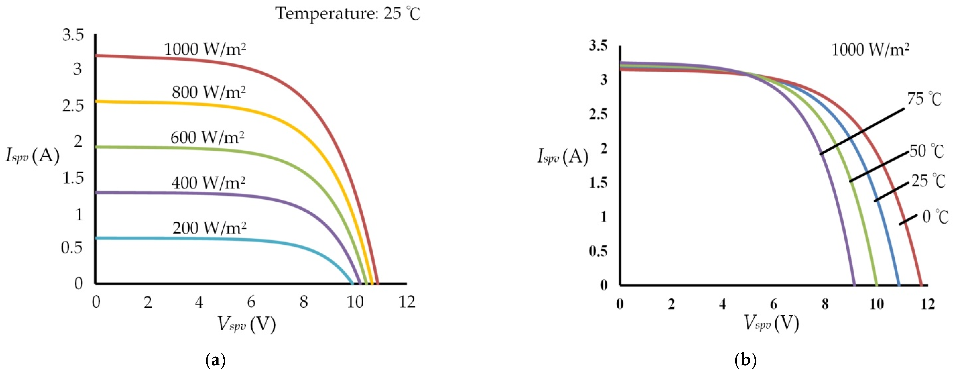
The SPV module (Everbright, model number Q025) was used during the experiment.
Figure 1a shows the SPV module
Ispv-
Vspv characteristic curves of the T of 25 degrees and the G of 200, 400, 600, 800 and 1000 W/m
2.
Figure 1b shows the SPV module
Ispv-
Vspv characteristic curves of the G of 1000 W/m
2 and the T of 0, 25, 50 and 75 °C.
In this study, the proposed method (based on
Figure 1a,b
Ispv-
Vspv characteristic curves) converted the relationship between
Ispv and
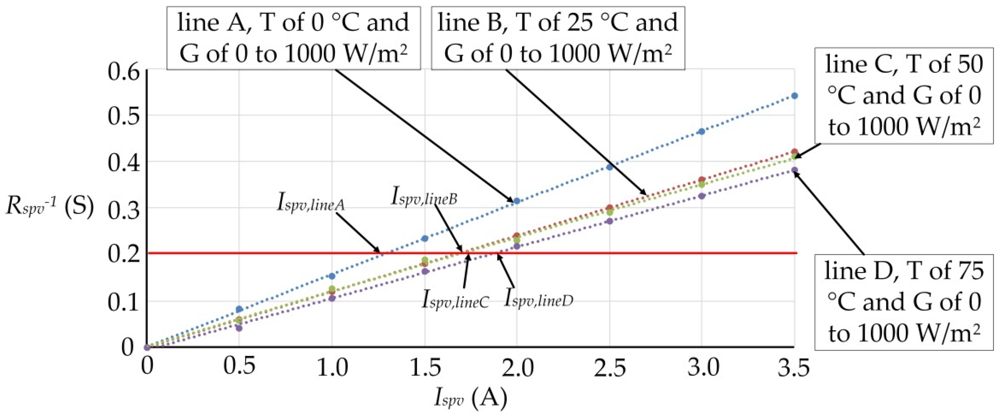
Rspv−1 through Microsoft Excel and presented it with trend lines. Hence, four trend lines were drawn (as in
Figure 2) to illustrate the relationship between
Ispv and
Rspv−1 as follows: line A for the T of 0 °C and the G of 0–1000 W/m
2, line B for the T of 25 °C and the G of 0–1000 W/m
2, line C for the T of 50 °C and the G of 0–1000 W/m
2 and line D for the T of 75 °C and the G of 0–1000 W/m
2. The mathematical model of the four trend lines could be approximated by the following quadratic equation, simplified as Equation (3).
Ispv is obtained by Equation (3) as follows:
In
Figure 2, line A was drawn with Equation (3) where the parameters
a,
b and
c are −0.0007, 0.1572 and −0.0005, respectively. Line B was drawn with the parameters
a,
b and
c as 0.0002, 0.1197 and 0.00003, respectively. Line C was drawn with the parameters
a,
b and
c as −0.0013, 0.1204 and −0.0012, respectively. Line D was drawn with the parameters
a,
b and
c as −0.0001, 0.1112 and −0.0058, respectively.
When the G and T change, the corresponding points of
Rspv−1 and
Ispv range from line A to line D, as shown in
Figure 2. In this study,
Rspv−1 =
Pspv/
Vspv2, according to Equation (4), to calculate
Ispv,line (e.g.,
Ispv,lineA,
Ispv,lineB,
Ispv,lineC and
Ispv,lineD). As shown in
Figure 2, when
Rspv−1 = 0.2 S,
Ispv,lineA,
Ispv,lineB,
Ispv,lineC and
Ispv,lineD are different. Although the four trend lines have the same
Rspv−1, a different T and G draw different trend lines and the calculated
Ispv,line will be significantly different.
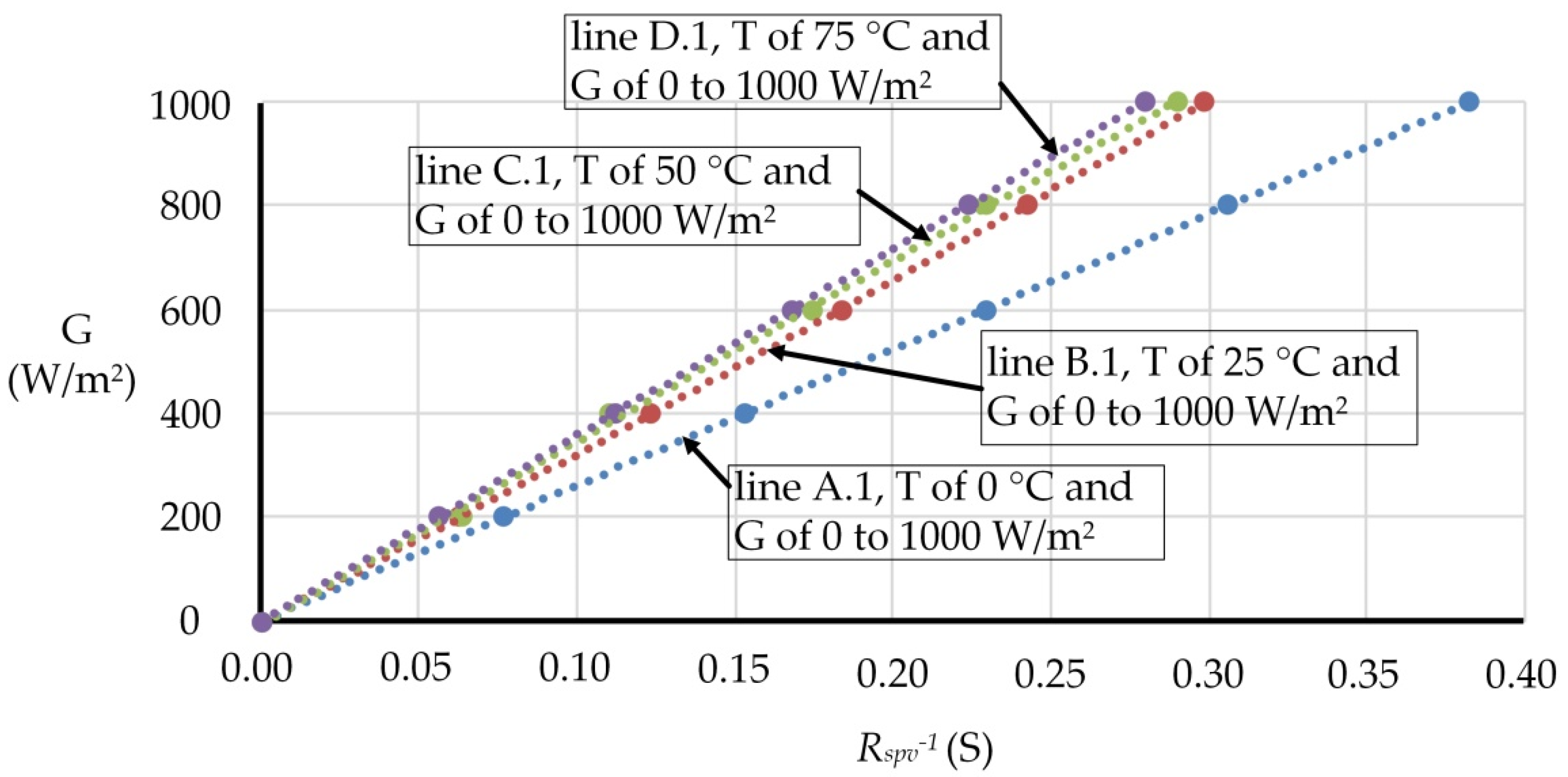
In this study, the proposed method, based on
Figure 1a,b
Ispv-
Vspv characteristic curves, converted the relationship between
Rspv−1 and the G through Microsoft Excel and presented it with trend lines. The four trend lines were drawn (as in
Figure 3) to show the relationship between the
Rspv−1 and the G as follows: line A.1 for the T of 0 °C and the G of 0–1000 W/m
2, line B.1 for the T of 25 °C and the G of 0–1000 W/m
2, line C.1 for the T of 50 °C and the G of 0–1000 W/m
2 and line D.1 for the T of 75 °C and the G of 0–1000 W/m
2. The mathematical model of the four trend lines could be approximated by the following quadratic equation, simplified as Equation (5):
In
Figure 3, line A.1 was drawn with Equation (5) using
d = 9 × 10
−11,
e = 2612.8 and
f = 2 × 10
−12; line B.1 was drawn with
d = 662.46,
e = 3148.2 and
f = −0.2585; line C.1 was drawn with
d = −232.85,
e = 3541.1 and
f = −5.7651 and line D.1 was drawn with
d = 6 × 10
−11,
e = 3575.5 and
f = −5 × 10
−13.
Figure 2 and
Figure 3 have a corresponding relationship between each other. If the values of
Rspv−1 and
Ispv fall on line A in
Figure 2, they correspond with line A.1 in
Figure 3 and then the G can be calculated by Equation (5). Furthermore, if the values of
Rspv−1 and
Ispv fall on line B or C or D in
Figure 2, they correspond with line B.1 or C.1 or D.1 in
Figure 3, respectively, and then the G can be calculated by Equation (5).
The proposed algorithm can calculate the G to improve the MPPT range and accuracy. Equation (5) is derived from Equations (2)–(4) and
Figure 1a,b. Therefore, the proposed algorithm under a different G and T can accurately track the MPP and improve the MPPT performance.
A comparison of the four trend lines in
Figure 3 shows that (1) the mean deviations of line A and line B were 6%, the mean deviations of line B and line C were 0.5% and the mean deviations of line C and line D were 1.8%; (2) assuming
Ispv > 1.06·
Ipv,lineB, it falls in the interval of line A; (3) if
Ispv ≦ 0.94·
Ispv,lineA or
Ispv > 1.005·
Ispv,lineC, it falls in the interval of line B; (4) assuming
Ispv ≦ 0.995·
Ispv,lineB or
Ispv > 1.018·
Ispv,lineD, it falls in the interval of line C; (5) assuming
Ispv ≦ 0.982·
Ispv,lineC, it falls in the interval of line D.
In order to determine the sudden change of G, the proposed algorithm used a continuous detection G variation value (dG). Generally, a sudden change in G is small in magnitude (smaller than 27 W/m
2) [
25]. In this control scheme judgment, G does not change, which reduces unnecessary vibrations of the actuating point. Therefore, in this study, the CTC threshold value was set to 27 W/m
2. Once the G change was detected to be more than 27 W/m
2, the proposed algorithm tracked the new MPP.
The designer’s actual demand sets the value of the CTC threshold. If the value of the CTC threshold is too small, the response is fast and the actuating point oscillations around the MPP cause power loss. On the contrary, when the value of the CTC threshold is too large, the response is slow and the MPPT will lack precision.
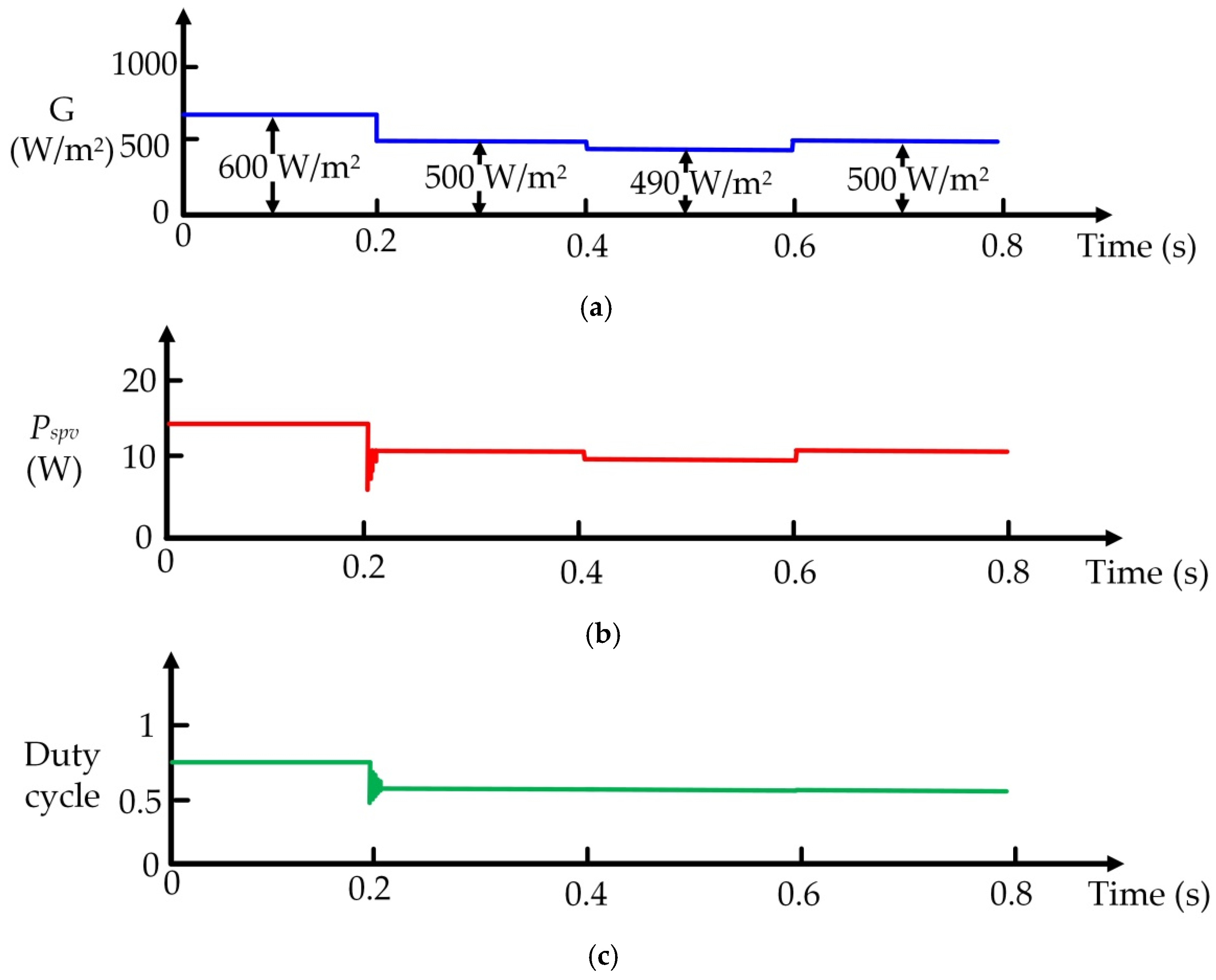
Figure 4a illustrates that when time = 0 s, there is a G of 600 W/m
2,
Pspv = 12 W and a duty cycle of 0.7, then when time = 0.2 s, the G of 600 W/m
2 drops to 500 W/m
2. Thus, the G variation value is more than 27 W/m
2. Therefore, the proposed algorithm starts to track the new MPP. The
Pspv of 10 W and duty cycle of 0.6 are shown in
Figure 4b,c.
Figure 4a displays that when time = 0.4 s, the G of 500 W/m
2 drops down to 490 W/m
2. Thus, the G variation value is less than 27 W/m
2. Therefore, the proposed algorithm to calculate the duty cycle is fixed, preventing perturbations that cause power loss. The
Pspv of 9.8 W and the duty cycle of 0.6 are shown in
Figure 4b,c.
Figure 4a illustrates that when time = 0.6 s, the G increases from 490 W/m
2 to 500 W/m
2. Thus, the G variation value is less than 27 W/m
2 and that the duty cycle is also fixed. The
Pspv of 10 W and duty cycle of 0.6 are shown in
Figure 4b,c.
The change in the Rspv of the SPV module is an important factor for MPPT. This proposed algorithm not only detects the SPV Module Pspv-Vspv characteristic curves but also utilizes the CTC based on Rspv to track the MPP. Furthermore, the proposed algorithm is suitable for poor climates (e.g., rain, cloud and shadow).
Figure 5 shows the proposed algorithm flowchart. First, the proposed algorithm implements the P&O algorithm, then reaches MPP; the duty cycle is fixed. Secondly, the proposed algorithm enters the CTC threshold control where
dVspv(n) =
Vspv(n) −
Vspv(n − 1);
dPspv(n) =
Pspv(n) −
Pspv(n − 1); the present SPV module output current is
Ispv; the present solar radiation is G; dG = |G(n) − G(n − 1)|;
a,
b and
c are the parameters of Equations (3) and (4) and
d,
e and
f are the parameters of Equation (5).
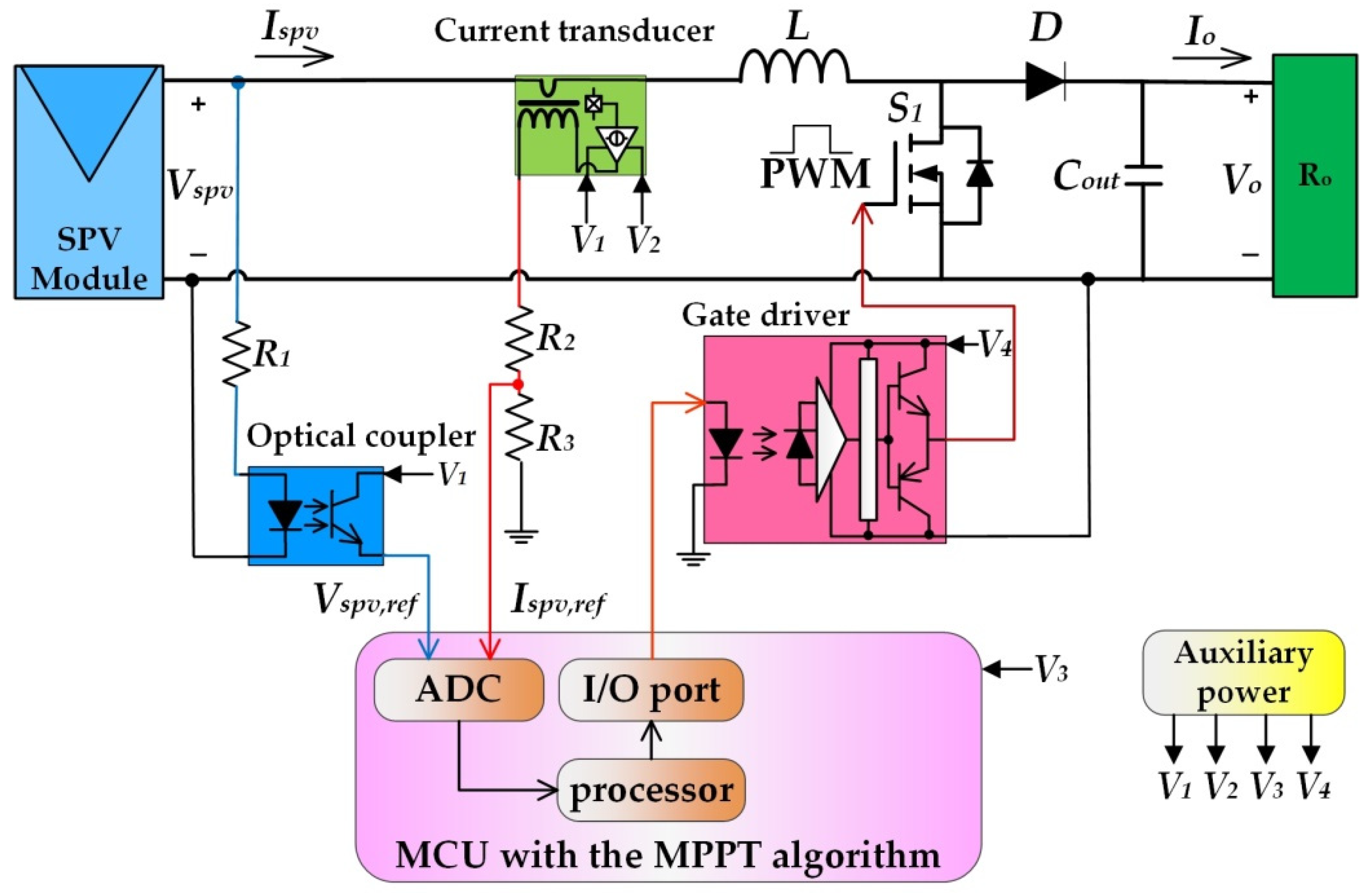
Figure 6 illustrates the boost converter with the MPPT algorithm-embedded diagram [
26]. Its main elements include an inductor (
L of 1 mH), a power MOSFET (
S1), a diode (
D) and a capacitor (
Cout of 220 μF). It includes feedback circuits of an optical coupler and a current transducer. Further, it detects the
Vspv and
Ispv and transmits the signals to the microcontroller unit (MCU). The MCU (Microchip Technology, model number 18F452) outputs the PWM signal (PWM frequency of 30 kHz) and then drives the gate driver to control
S1 and reach the MPP.
4. Experimental Results
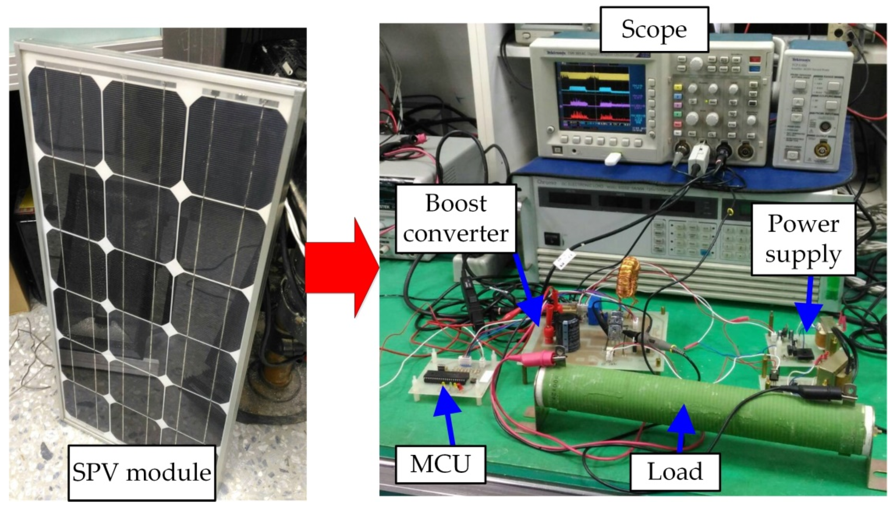
Figure 7 shows the experimental SPV module and the prototype setup. The SPV module (model number Q025, Everbright, Beijing, China) G of 1000 W/m
2 and T of 25 °C specifications are as follows:
VMPP = 8.3 V,
IMPP = 2.4 A and
PMPP = 20 W. In this experiment, the SPV module output power was connected to the input of the boost converter and the boost converter output was connected to the load. The MCU was employed to perform the MPPT control. The MCU outputted the PWM signal to drive the boost converter power MOSFET,
S1, which then reached the MPP.
In order to verify the proposed algorithm and the P&O algorithm performance, this study ran an experimental test under varying solar radiation and partial shading conditions. The results of the experimental proposed algorithm performance were higher than the P&O algorithm (
Figure 8 and
Figure 9).
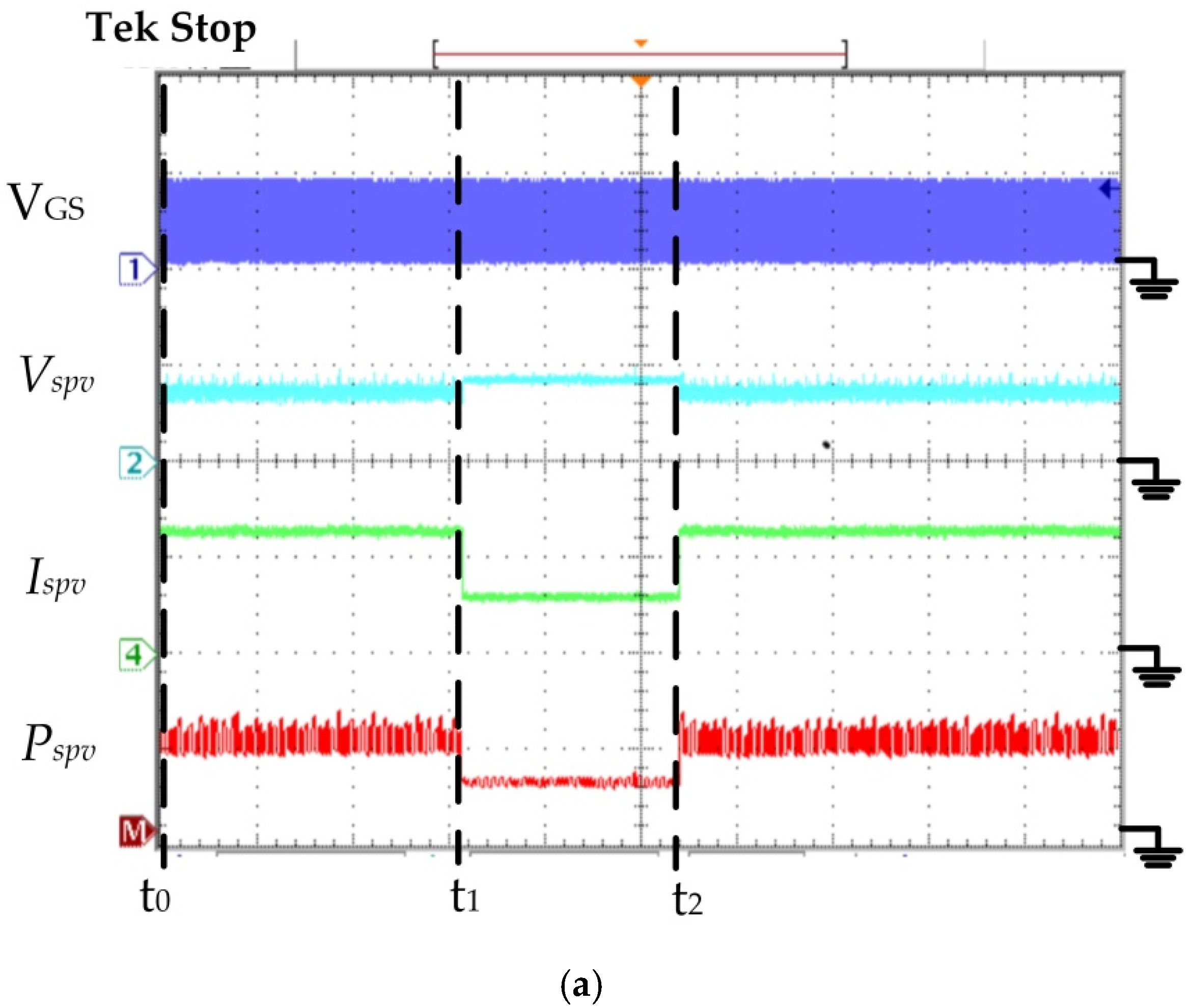
Figure 8 displays the comparison between the proposed algorithm and the P&O algorithm test results when the varying irradiance of 500 W/m
2 dropped to 220 W/m
2 then increased to 500 W/m
2 with a T of 25 °C.
Figure 8a shows that the proposed algorithm’s MPPT was activated. When time = t
0, the SPV module
Rspv−1 = 0.154 S,
Vspv = 8.5 V,
Ispv = 1.32 A and
Pspv = 11.22 W. According to Equation (4), the following were calculated:
Ispv,lineA,
Ispv,lineB,
Ispv,lineC and
Ispv,lineD, respectively. The
Ispv,lineC = 1.299 A and
Ispv > 1.005·
Ispv, lineC. Thus, the
Ispv fell on line B (
Figure 2), which corresponded with line B.1 (
Figure 3). Equation (5) was used to calculate the G = 500 W/m
2. At time = t
1, the SPV module
Rspv−1 = 0.072 S,
Vspv = 8.5 V,
Ispv = 0.62 A and
Pspv = 5.3 W. According to Equation (4), the following were calculated:
Ispv,lineA,
Ispv,lineB,
Ispv,lineC and
Ispv,lineD, respectively. The
Ispv,lineC = 0.6 A and
Ispv > 1.005·
Ispv,lineC. Therefore, the
Ispv fell on line B (
Figure 2), which corresponded with line B.1 (
Figure 3). Equation (5) was used to calculate the G = 220 W/m
2. At time = t
2, the SPV module
Rspv−1 = 0.154 S,
Vspv = 8.5 V,
Ispv = 1.32 A and
Pspv = 11.22 W. According to Equation (4), the following were calculated:
Ispv,lineA,
Ispv,lineB,
Ispv,lineC and
Ispv,lineD, respectively. The
Ispv,lineC = 1.299 A and
Ispv > 1.005·
Ispv,lineC. Thus, the
Ispv fell on line B (
Figure 2, which corresponded with line B.1 (
Figure 3). Equation (5) was used to calculate the G = 500 W/m
2. The proposed algorithm could accurately calculate the G and adjust the duty cycle track to the MPP. When the G was constant, the duty cycle was fixed. Therefore, the proposed algorithm caught the MPP accurately.
Figure 8b displays the P&O algorithm test results. This algorithm’s MPPT was activated and perturbed to track the MPP and then the perturb method resulted in power loss. When the P&O algorithm at time = t
0 and a G of 500 W/m
2, at time = t
1, the G of 500 W/m
2 dropped to 220 W/m
2 and at time = t
2, the G of 220 W/m
2 rose to 500 W/m
2. The experiment results verified that the proposed algorithm’s MPPT efficiency was better than the P&O algorithm (as in
Table 1).
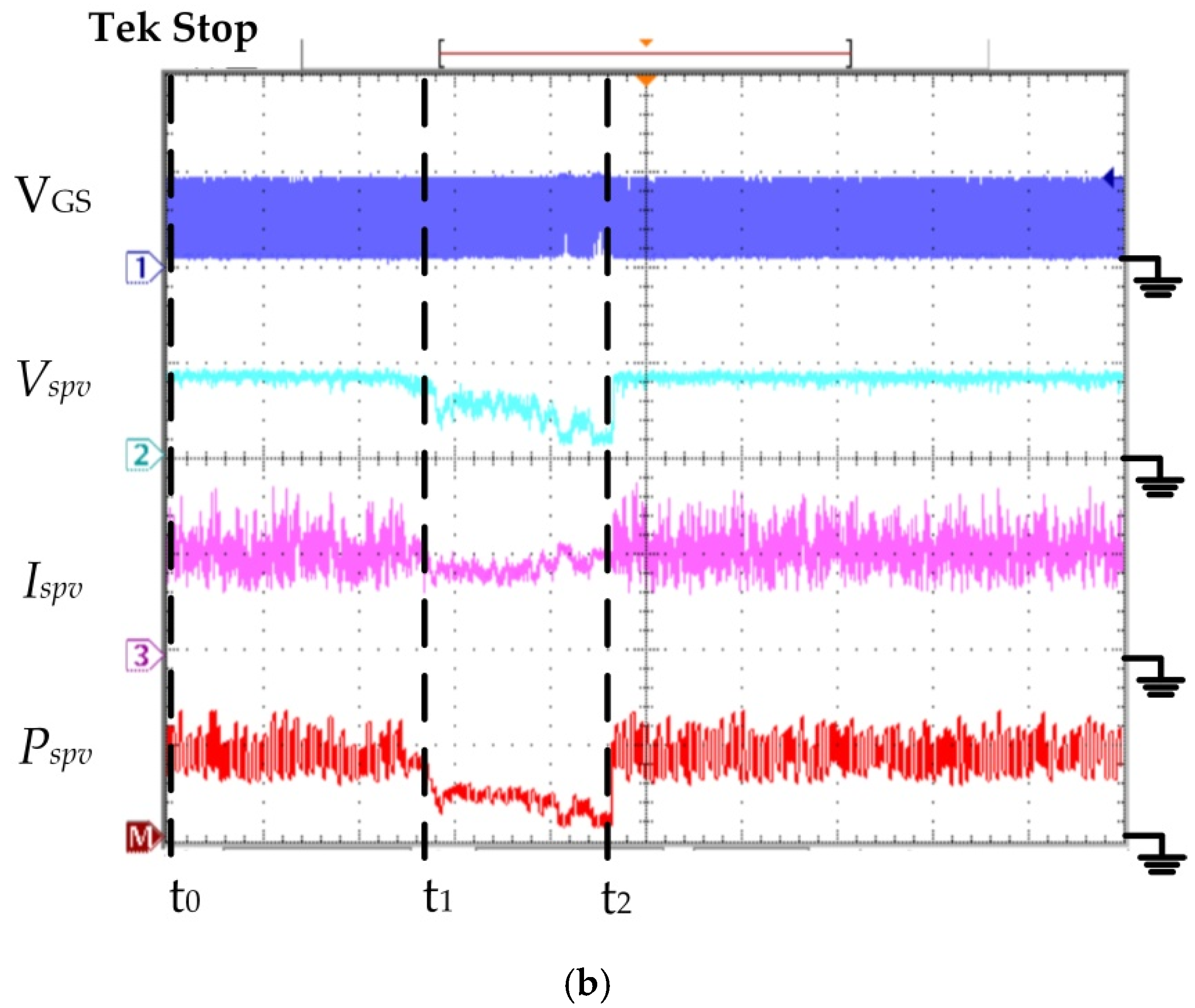
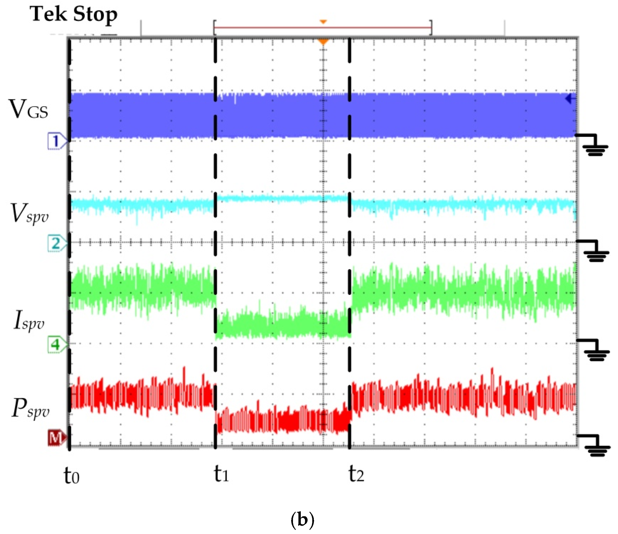
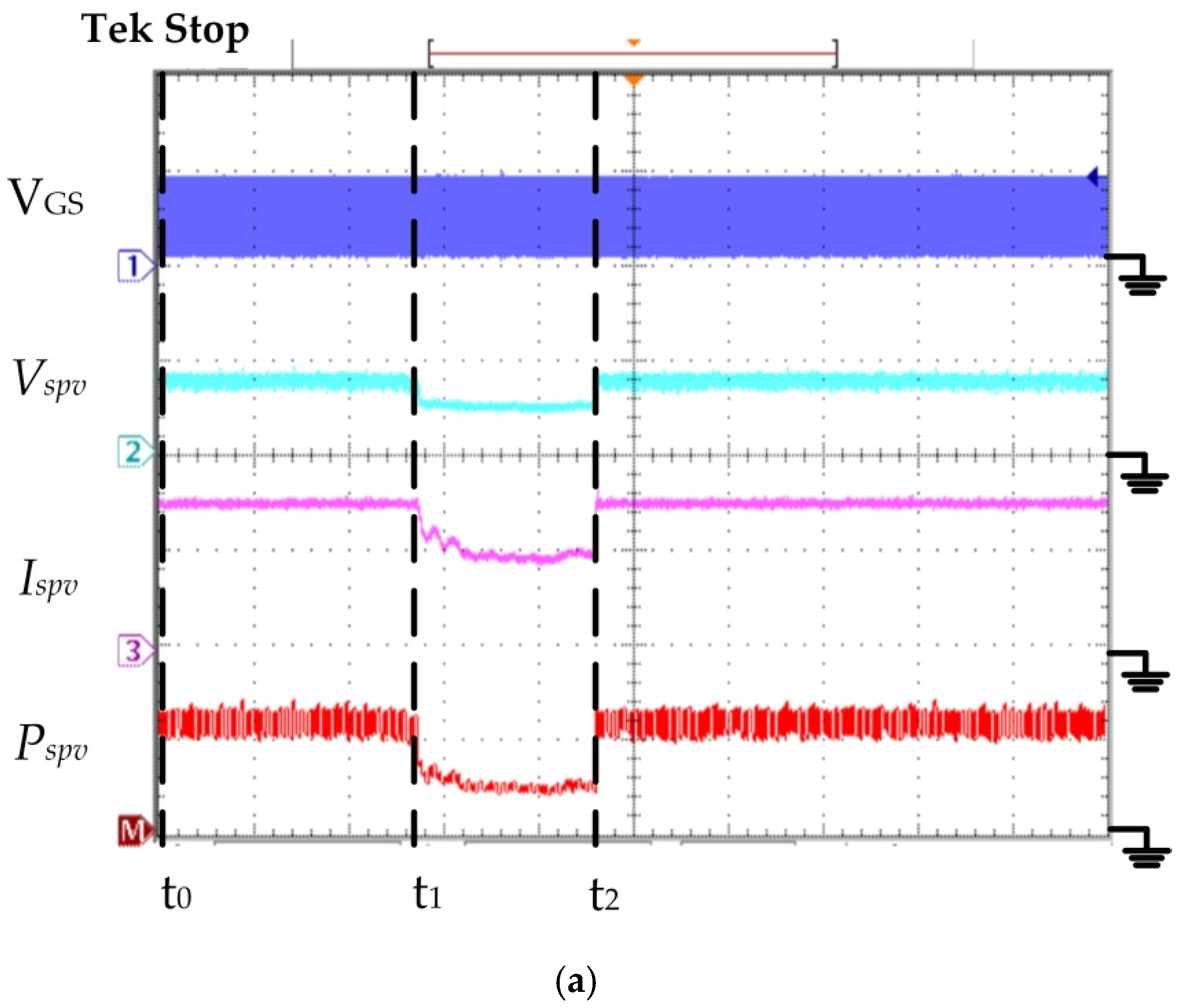
Figure 9 shows the comparison between the proposed algorithm and the P&O algorithm test results in partial shading conditions. The G and T were respectively 540 W/m
2 and 25 °C.
Figure 9a shows that the proposed algorithm MPPT was activated. When the proposed algorithm at time = t
0, the SPV module
Rspv−1 = 0.166 S,
Vspv = 9 V,
Ispv = 1.5 A and
Pspv = 13.5 W. According to Equation (4), the following were calculated:
Ispv,lineA,
Ispv,lineB,
Ispv,lineC and
Ispv,lineD, respectively. The
Ispv,lineC = 1.41 A and
Ispv > 1.005·
Ispv,lineC. Therefore,
Ispv fell on line B (
Figure 2), which corresponded with line B.1 (
Figure 3). Equation (5) was used to calculate the G = 540 W/m
2. At time = t
1, the SPV module suffered 1/2 partial shading conditions
Pspv = 6 W. The proposed algorithm was provided by the P&O algorithm with a quick response and accurately calculated the G and adjusted the duty cycle track to the MPP. When the G was constant, the duty cycle was fixed. Therefore, the proposed algorithm stably caught the MPP. At time = t
2, the SPV module
Rspv−1 = 0.166 S,
Vspv = 9 V,
Ispv = 1.5 A and
Pspv = 13.5 W. According to Equation (4), the following were calculated:
Ispv,lineA,
Ispv,lineB,
Ispv,lineC and
Ispv,lineD, respectively. The
Ispv,lineC = 1.41 A and
Ispv > 1.005·
Ispv,lineC, so
Ispv fell on line B (
Figure 2), which corresponded with line B.1 (
Figure 3). Equation (5) was used to calculate the G = 540 W/m
2. Similarly, the proposed algorithm caught the MPP accurately.
Figure 9b shows the P&O algorithm test results. This algorithm’s MPPT was activated and perturbed to track the MPP. However, the perturb method could converge to the LPPP, resulting in a lower system efficiency. When the P&O algorithm at time = t
0 and G of 540 W/m
2, at time = t
1, the SPV module suffered 1/2 partial shading conditions
Pspv = 4.7 W and at time = t
2, a G of 540 W/m
2. Similarly, the experiment results verified that the proposed algorithm’s MPPT efficiency was higher than the P&O algorithm (as in
Table 1).


