Effects of Dynamic Pricing on the Design and Operation of Distributed Energy Resource Networks

Abstract

This paper presents a framework for the use of variable pricing to control electricity imported/exported to/from both fixed and unfixed residential distributed energy resource (DER) network designs. The framework shows that networks utilizing much of their own energy, and importing little from the national grid, are barely affected by dynamic import pricing, but are encouraged to sell more by dynamic export pricing. An increase in CO₂ emissions per kWh of energy produced is observed for dynamic import and export, against a baseline configuration utilizing constant pricing. This is due to feed-in tariffs (FITs) that encourage CHP generation over lower-carbon technologies. Furthermore, batteries are shown to be expensive in systems receiving income from FITs and grid exports, but for the cases when they sell to/buy from the grid using dynamic pricing, their use in the networks becomes more economical.

1. Introduction

In 2016, the UK received 24.5% of its electricity generation from renewable technologies, with further 46.2% coming from low carbon systems [1]. Most electricity in the UK grid comes from large producers located far from customers, e.g., large offshore wind farms or isolated nuclear plants. This leads to enormous volumes of electricity wasted through transmission losses and step-up/step-down transformers [2].

This reality has raised the incentive to research different ways to provide more economical and environmentally friendly electricity production. Many authors have generated various MILP models to demonstrate the potential of distributed energy resource (DER) systems to provide both domestic and commercial buildings with greater local, self-generated energy from renewable or low carbon assets. This will be able to mitigate much of these transmission losses and, consequently, reduce carbon emissions and energy bills [3,4,5,6,7].

Much work into this area exploits the fact that many governments are willing to pay users to consume self-generated, low-carbon electricity and heat, through Feed-in tariffs (FITs), and renewable heat incentives (RHIs). They will also pay for these units to export excess electricity to the wider national grid [8,9], a good case for homeowners and businesses to invest in DER technologies. However, while such investment would help meet national CO₂ reduction targets, accompanied by money saving for customers, large-scale investment into domestic DERs without sensible controls could destabilize national grid structures. The reason for this being that many already deal with various large-scale renewable assets intermittently feeding into it, not necessarily at times of demand [10]. This forces grid operators to ask large non-renewable plants to start-up and shut-down operation without much warning, makes grid balancing difficult and expensive, and leads to increased costs for the consumers.

Accordingly, to make residential DERs compatible with the national grid, a control strategy is needed which encourages renewable asset owners to generate, consume, store and sell energy at times which are mutually beneficial to them and ensure the stability of the national grids.

The IoT concept is defined as a group of infrastructures interconnecting connected objects and allowing their management, data mining and the access to the data they generate [11]. The IoT technologies have the potential to better control and optimize DERs in conjunction with the needs of the national electricity grids, by providing a sustainable solution for the dynamic management of the system. This can be done through internet connected controllers which utilize live data on energy prices, generation, consumption, and asset failures, in a manner aligned with national grid strategies. They also present the capability to optimize the design and operation of local renewable resources to cope with predicted changes in weather or disruptive events.

One strategy which has been proposed to help stabilize national grids is the use of dynamic pricing, as discussed in Finn and Fitzpatrick [12]. Dynamic pricing is a strategy in which national grids publish, either in real time, or a few days ahead, variable prices per kWh of electricity, within a given time period. For example, one might make 06:00–08:00 P.M. on a winter’s day an expensive time in which to consume energy, because this is a time of high demand, when many homeowners cook dinner and/or watch television. The effect of this would be that large-scale consumers, for example chemical processing plants, might cut back operation during this period to save money, and recover the lost production when electricity demand is much lower and the consumption is encouraged by the grid through a lower cost per unit of electricity, for example at 02:00 A.M.

Without automated optimization of such variable operation, only a few large industrial users will likely modify their usage to accommodate such a strategy. It has been suggested that dynamic pricing could be employed in smart homes [13], where, for example, electric vehicles would be charged overnight when electricity is cheap and dish washers would only turn on in the early hours of the morning, when the IoT controller tells them to, in accordance with user pre-set requirements.

This strategy could also be flipped on its head and used to encourage renewable resources within an IoT controlled residential DER network (e.g., wind turbines (WTs), solar cells, battery storage etc.) to sell electricity to the grid during peak national demand, when the sale price is high, and to store renewable power, in battery units, when the sale price is low [10]. These two routines would help flatten the demand profile throughout the day (or perhaps even the year) and simplify the balancing of demand and supply for the grid operators, and could even reduce the voltage used on national grids since peak volumes of energy could be reduced.

Dynamic pricing could be used to reflect the needs of the grid, in a process known as Demand Side Management [12], which can be a function of the time of day, week and year, as well as weather conditions and public demand. Pricing variations of imports and exports could also reflect the failure of large assets, e.g., emergency shut-down of a large coal or nuclear asset, or changes in legislation of FIT and RHI pricing.

This could better enable grid actors to deal with blackouts and possibly minimize the size of the affected areas during such events. The IoT controllers could also use big data capabilities to learn more about end-user’s operation, which would better inform the grid on the generation and demand profiles, and enable the integration of multiple local grids that support each other, possibly even trading energy between one another [10].

While much has been hypothesized about the potential of IoT to stabilize grid operations, in a Smart Grid [10] or The Enernet, the inevitable convergence of the smart grid with the IoT [14], little has been done to quantify the possible effects, either using optimization models or through real-world implementation.

Xu et al. [10] have presented a statistical study to evaluate the differences in cost per kWh and the reliability between three types of national grid structures, namely:

(1)

The current typical structure in which the electricity is generated in large industrial units, far from end users;

(2)

A grid with integrated DERs; and

(3)

A grid with integrated DERs and battery storage units. With respect to the end-user energy costs, the findings were that the DER integrated network is cheaper than the traditional grid.

Furthermore, battery storage introduces greater reliability to the network, albeit at a greater cost [10]. This reflects the findings of authors who have written solely about residential DER design optimization. Wouters et al. [7], for example, found that battery storage was not economically viable for residential DERs in South Australia.

The work presented in the following sections focuses on the use of IoT-type integration and communication strategies for the control of residential DERs, as opposed to the control of entire grids, as presented by Xu et al. [10]. With respect to dynamic pricing, the paper is unique from the work of Finn and Fitzpatrick [12], in that it investigates both demand- and supply-side control, with focus on residential housing as opposed to industrial buildings. Furthermore, it also expands on the potential use of batteries and investigates the maximum cost at which batteries become economical under various scenarios, thus giving greater insight into their use than previous models which have simply stated that they are not economical [7].

Finally, the framework presented here builds on the capabilities of those presented by Mechleri et al. [6] and Wouters et al. [7], by expanding the models in terms of different types of technologies used and also the different approaches for the case studies, and builds on the preliminary results presented in [15].

The remainder of the paper is split into the following: Section 2 describes the methodology followed in this work, Section 3 reports the results of the various scenarios considered, while Section 4 focuses on the conclusions. Finally, the Appendix includes a glossary of technical terms and the appendices which contain detailed data used for the MILP model.

2. Methodology

A baseline scenario, with a pre-designed DER network is used to investigate the effects of dynamic pricing. An optimization problem is formulated for the design of the network without dynamic pricing, based on several available renewable technologies. The set of candidate technologies (Tech) are:

• Absorption chillers (Abs);
• Air conditioning units (AC);
• Biomass boilers (BB);
• Gas boilers (GB);
• Combined heat and power generators (CHP), which can be fuel cells, internal combustion engines or Sterling engines;
• Gas heaters (GH);
• Heating/cooling pipelines (PLs);
• Microgrid controllers (MGCC);
• Photovoltaic cells (PV);
• Thermal storage (TS);
• Wind turbines (WTs).

A second scenario is investigated where the design of the network is done considering dynamic pricing control strategies. The two scenarios are then compared to evaluate the contribution of the dynamic pricing in the design of the network.

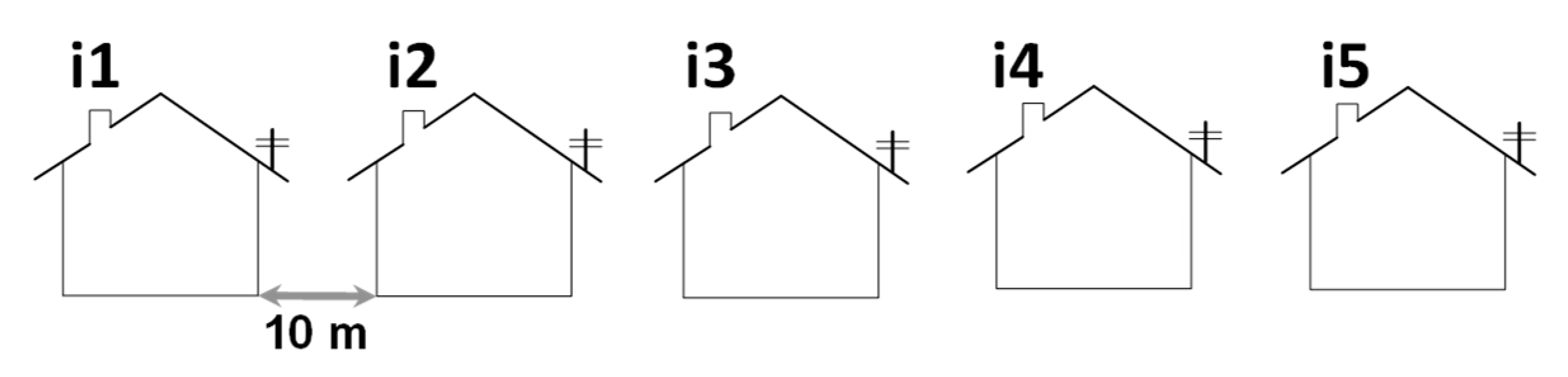
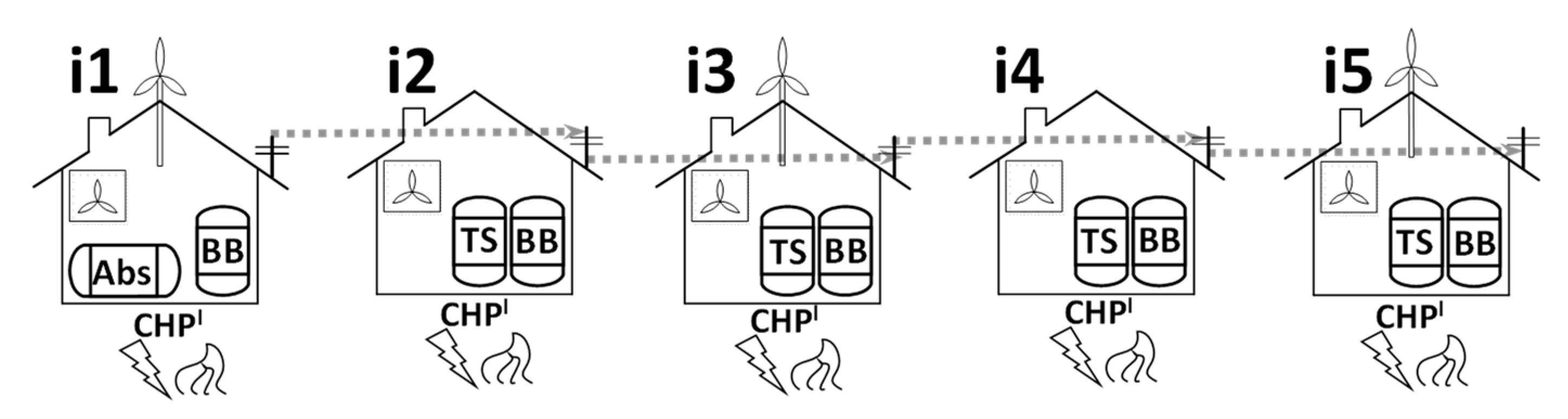
A case study [15] is used to illustrate the approach: a residential house arrangement based on streets in Guildford, Surrey, UK, with five (5) houses (Figure 1), numbered i1–i5 and spaced 10 m apart. This spacing represents the lengths that would be needed to make connections via pipelines (PLs) or microgrid (MG) cables.

Figure 1. The five-house neighborhood.

The homes can generate heating, cooling, domestic hot water (DHW) and/or electrical power to meet their own demands but also the needs of the other homes in the network, transmitted via pipelines and MG cables. Excess electricity generated can be sold to the national grid and electricity and gas imported from the grid, at a price, to the network.

Although the application is demonstrated on a UK case study, the framework can be applied easily to scenarios for other countries by replacing sizes and costs of technologies, as well as demands, pricing or policy-related costs, as required by the local situation.

2.1. Seasonal and Hourly Variations in Supply and Demand (Multiperiod Operation Discretization)

Real seasonal and hourly variations in supply and demand of the various energy requirements and renewable generating assets are considered for the models, as discussed in [15]:

(1)

UK weather and demand data is split into four seasons: m1—spring; m2—summer; m3—autumn; and m4—winter, which each lasts for three months, March–May, June–August, September–November, and December–February, respectively.

(2)

Each month within a season has the same number of days, taken as the average of the three months: m1 = 31; m2 = 31, m3 = 30, m4 = 30.

(3)

Furthermore, every day is split into six time periods, p1 to p6, in which demand, weather operation and thus renewable energy supply are constant.

The length and the start and end times for each of the six time periods are shown in Table 1.

Table 1. Time periods used in the model.

Time Period (p)	p1	p2	p3	p4	p5	p6
Duration [h]	2	3	1	5	4	9
Start time	07:00	09:00	12:00	13:00	18:00	22:00
End time	09:00	12:00	13:00	18:00	22:00	07:00

The information on weather data considered for the model are shown in Table 2 and Table 3.

Table 2. UK solar insolation data (adapted from [16]).

Time Period (p)	p1	p2	p3	p4	p5	p6
Month	Solar Insolation [kW]
m1	0.155	0.375	0.420	0.235	0.002	0.000
m2	0.320	0.485	0.525	0.355	0.033	0.000
m3	0.150	0.380	0.420	0.240	0.003	0.000
m4	0.033	0.170	0.208	0.070	0.000	0.000

Table 3. UK wind speed data (adapted from [16]).

Time Period (p)	p1	p2	p3	p4	p5	p6
Month	Wind Speed [m/s]
m1	5.90	6.25	7.70	7.80	6.25	5.90
m2	5.00	5.60	6.00	6.30	5.70	4.80
m3	6.85	6.30	6.70	6.80	6.25	5.90
m4	6.60	6.70	6.90	7.05	6.70	6.15

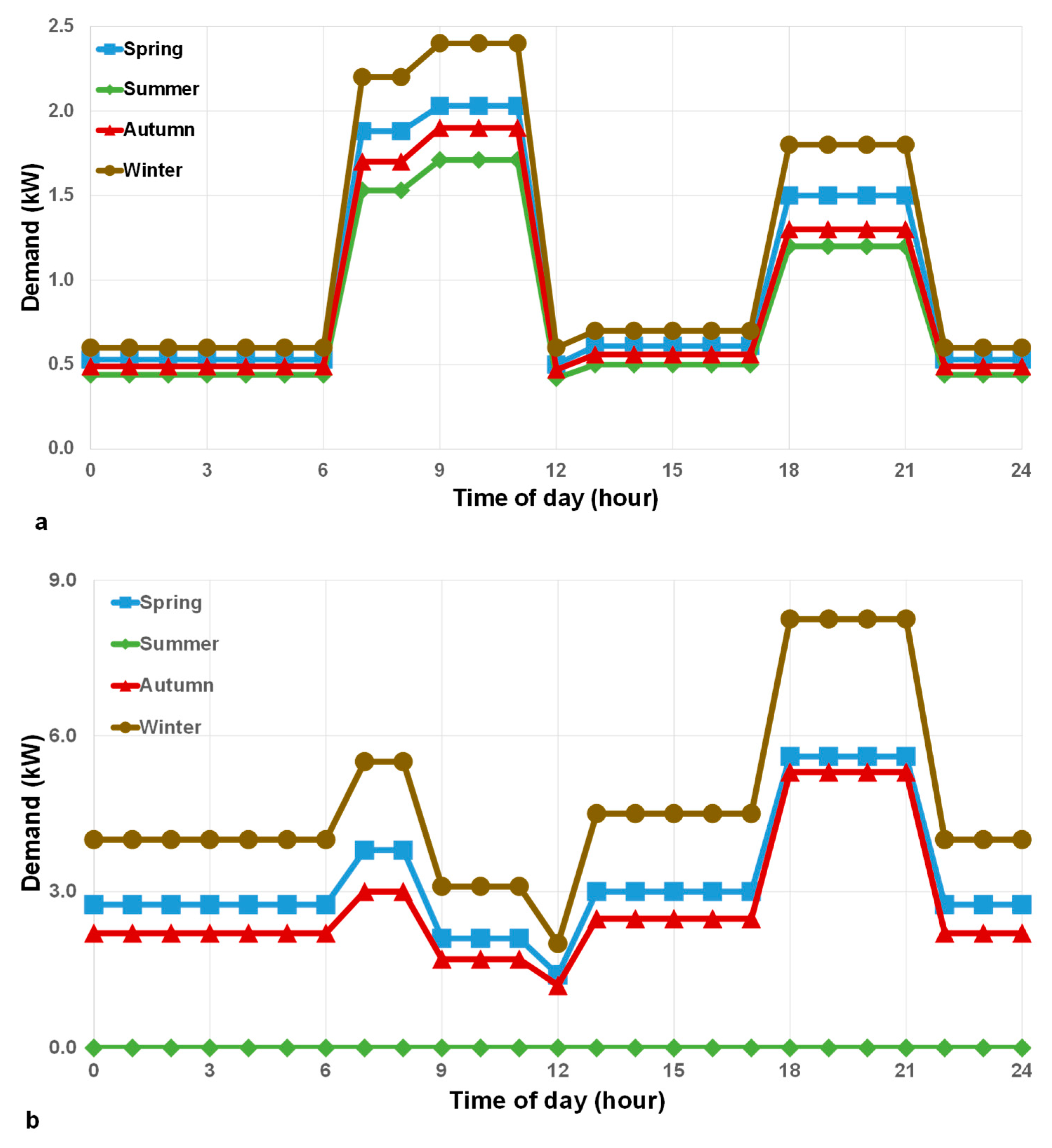
The demand profiles considered for all utilities can be seen, as a function of the time of day and season, in Figure 2, constructed from data in [4,16,17,18,19]. A representative day for each season (Spring, Summer, Autumn and Winter) is chosen in determining the demand profiles.

Figure 2. Average demand profiles per household for (a) electricity (adapted from [4] and [16]); (b) heating (adapted from [4,19]); (c) cooling (adapted from [17,18]); and (d) hot water (adapted from [4,19].

A scalar is considered for each house (Table 4) that is used to define five different demand profiles for each utility at any one time.

Table 4. Scalars used to obtain demand profiles for each house in the network.

House	i1	i2	i3	i4	i5
Scalar	0.8	0.9	1.0	1.1	1.2

It is ensured that using the five scalars, the average demand per household for each utility is the one defined in Figure 2.

2.2. Mathematical Formulation

A simplified version of the model was previously described in [15]. In the following sections, the mathematical formulation, with all equations and assumptions will be presented in more detail.

2.2.1. Objective Function

The model’s objective function minimizes the annualized cost of the energy network ($C_{Total}$). The total cost is calculated as the sum, for all technologies, of the investment costs ($C_{Inv}^{Tech}$) annualized over the project lifetime (n) and the annual operating and maintenance costs ($C_{O\&M}^{Tech}$), the annual cost of carbon emission taxation ($C_{Tax}^{Tech}$), the annual cost of imported energy and fuel ($C_{Fuel}^{Tech}$), minus the annual income ($C_{Income}^{Tech}$) made from exporting electricity to the grid, feed in tariffs (FITs) and renewable heat incentives (RHIs), as shown in Equation (1):

$$C_{Total}={{\displaystyle \sum }}_{Tech}\left(C_{Inv}^{Tech}+C_{O\wedge M}^{Tech}\right)+C_{Tax}^{Tech}+C_{Fuel}^{Tech}-C_{Income}^{Tech}$$

(1)

2.2.2. Annualized Investment Costs

The annualized investment costs are calculated based on a capital recovery factor (CRF) using the interest rate, r (%), and the project lifetime, n (years). For all technologies, the values of r and n are kept constant and based on the values available from similar investigations ([6,7,20,21,22,23]), allowing for ease of comparison between different technologies, scenarios and research conditions:

$$CRF=\frac{r·{\left(1+r\right)}^n}{{\left(1+r\right)}^n-1}$$

(2)

The investment cost of the installed capacity can be calculated as:

$$C_{Inv}^{Tech}={{\displaystyle \sum }}_i\left(CRF·C_{capital}^{Tech}·Ge{n}_{Max,i}^{Utility,Tech}\right)$$

(3)

Here, $Ge{n}_{Max,i}^{Utility,Tech}$ is the maximum amount of Utility generated by the technology Tech in a house i, in a year. The following utilities are considered: electricity (E), space heating (H) and cooling (C), and domestic hot water (DHW). Hence $Ge{n}_{Max,i}^{Utility,Tech}$ represents the required installed capacity of the technology Tech and must be at least equal to or greater than the highest yearly demand:

$$Ge{n}_{Max,i}^{Utility,Tech}>Ge{n}_{i,m,p}^{Utility,Tech}\forall Ge{n}_{i,m,p}^{Utility,Tech}\ne Ge{n}_{Max,i}^{Utility,Tech}$$

(4)

The installed capacity of the technologies Tech is bounded by upper and lower bounds of typically available equipment:

$$\begin{array}{l}Ge{n}_{Max,i}^{Utility,Tech}\ge L{B}^{Tech}·Y_i^{Tech}\\ Ge{n}_{Max,i}^{Utility,Tech}\le U{B}^{Tech}·Y_i^{Tech}\end{array}$$

(5)

Here, $Y_i^{Tech}$ is a binary variable which decides if a technology Tech is placed in a home i.

Equations (4) and (5) apply to all technologies Tech presented at the beginning of Section 2. In case of the photovoltaic network, the investments are calculated based on the installed surface area of the panels. Furthermore, the electricity generation from PV cells is a function of the solar irradiance, $SI{r}_{m,p}$, which varies with the time of day and season, the surface area installed, $A_i^{PV}$, which is an optimisation variable, and the panel efficiency, ${\eta }^{PV}$, a set parameter:

$$Ge{n}_{i,m,p}^{E,PV}\le A_i^{PV}·SI{r}_{m,p}·{\eta }^{PV}$$

(6)

The generation from the PV cells is also a function of the rated panel capacity, RPC:

$$Ge{n}_{i,m,p}^{E,PV}=RPC·A_i^{PV}$$

(7)

In case of the WTs, the investments costs are based on the number of turbines installed and not on the capacity. The maximum capacity is set to 1.5 kW and is equal with the rated capacity, as used in [24]. Furthermore, it was decided that it was impractical to have WTs in adjacent houses, hence a rule was put in place that there must be at least a one house gap between WT installations:

$$Y_{i+1}^{WT}+Y_i^{WT}\le 1$$

(8)

Finally, for the sake of space within homes, only one CHP is permitted in each dwelling:

$${{\displaystyle \sum }}_{CHP}{Y}_i^{CHP}\le 1$$

(9)

In case of the network operation, the capital costs, $C_{capital}^{Tech}$ are calculated based on the length of the cable or pipe installed. Furthermore, for the batteries, besides the cost expressed by Equation (3) there is a secondary investment cost associated with the storage unit controller:

$$C_{Inv}^{controller,ES}=CRF·C_{capital}^{controller,ES}·{{\displaystyle \sum }}_i{Y}_i^{ES}$$

(10)

The capital cost of the microgrid controller is calculated from:

$$C_{Inv}^{MG}=C_{capital}^{controller,MG}·Z$$

(11)

With Z being a binary variable which determines the existence of the microgrid.

2.2.3. Operating and Maintenance Costs

The operating and maintenance (O&M) costs, $C_{O\&M}^{Tech}$, of the technologies Tech are calculated using fixed and variable costs, as used in other case studies ([6,7,20,21,22,23]):

$$C_{O\&M}^{Tech}={{\displaystyle \sum }}_i\left[\begin{array}{c}\left(C_{OM,Fixed}^{Tech}·Ge{n}_{Max,i}^{Utility,Tech}\right)+\\ \left(C_{OM,Var}^{Tech}·{{\displaystyle \sum }}_{m,p}Ge{n}_{i,m,p}^{Utility,Tech}·day\left(m\right)·hours\left(p\right)·season\left(m\right)\right)\end{array}\right]$$

(12)

Finally, since the microgrid itself uses electricity it has an O&M cost as well:

$$C_{O\&M,CC}^{MG}=C_{OM}^{controller,MG}·Z$$

(13)

2.2.4. Environmental Costs

A tax is put in place by the UK government to penalize electricity generators for CO₂ emissions. The cost of carbon emission taxation, $C_{Tax}$, is calculated from the government tax of CO₂ emitted, $P_{C{O}_2}$, the carbon intensity of electricity purchased from the grid, $C{I}^{grid}$, and the carbon intensities of emitting technologies (gas boiler, CHP, gas heater). Given that all of these units consume natural gas, this can be considered as the carbon intensity of the grid gas, $C{I}^{gas}$, divided by the technology Tech’s efficiency, ${\eta }^{Tech}$:

$$C_{Tax}=P_{C{O}_2}·{{\displaystyle \sum }}_{Tech}\left[\begin{array}{c}\left(C{I}^{gas}·{{\displaystyle \sum }}_{i,m,p}\frac{Ge{n}_{i,m,p}^{Tech}}{{\eta }^{Tech}}·day\left(m\right)·hours\left(p\right)·season\left(m\right)\right)+\\ C{I}^{grid}·{{\displaystyle \sum }}_{i,m,p}{E}_{i,m,p}^{Grid}·day\left(m\right)·hours\left(p\right)·season\left(m\right)\end{array}\right]$$

(14)

where $E_{i,m,p}^{Grid}$ is the electricity purchased from the grid.

Accordingly, the CO₂ cost of the network is calculated by calculating the volume of CO₂ produced by each technology Tech throughout the year.

2.2.5. Costs of Fuel

The cost of fuel, $C_{Fuel}$ is equal to the volume of gas and electricity purchased multiplied by the respective cost of each:

$$C_{Fuel}=\left(\begin{array}{c}{P}_{Elec}·{{\displaystyle \sum }}_{i,m,p}{E}_{i,m,p}^{Grid}+\\ P^{gas}·{{\displaystyle \sum }}_{Tech}{{\displaystyle \sum }}_{i,m,p}\frac{Ge{n}_{i,m,p}^{Utility,Tech}}{{\eta }^{Tech}}\end{array}\right)·day\left(m\right)·hours\left(p\right)·season\left(m\right)$$

(15)

The cost of gas from the national grid is defined by $P^{gas}$ (£/ kWh).

2.2.6. Income

The income, $C_{Income}$, is calculated from the FITs per kWh of low carbon Utility generated, $P_{FIT}^{Tech}$, the electricity sales to the grid, $E_{Sale,i,m,p}^{Tech}$, and the annual payment for utilisation of a biomass boiler under the RHI, $P_{RHI}$. The electricity generated in the network, which exceeds network demands, can be sold to the national grid:

$$C_{Income}=\left(\begin{array}{c}{{\displaystyle \sum }}_{Tech}{P}_{Sale}^{Tech}·{{\displaystyle \sum }}_{i,m,p}{E}_{Sale,i,m,p}^{Tech}·day\left(m\right)·hours\left(p\right)·season\left(m\right)+\\ {{\displaystyle \sum }}_{Tech}{P}_{FIT}^{Tech}·{{\displaystyle \sum }}_{i,m,p}Ge{n}_{i,m,p}^{Utility,Tech}+{{\displaystyle \sum }}_i{P}_{RHI}^{BB}·Y_i^{BB}\end{array}\right)$$

(16)

To ensure that homes do not become power plants and are, in fact, only selling excess and not generating electricity purely for profit, a rule is put in place stating that the total electricity sold from all technologies Tech cannot exceed that generated by all units, minus the demand of the home:

$$\begin{gathered} {{\displaystyle \sum }}_{Tech}{E}_{Sale,i,m,p}^{Tech}\le \\ \left(\begin{array}{c}{{\displaystyle \sum }}_{Tech}Ge{n}_{i,m,p}^{E,Tech}+StoreOu{t}_{i,m,p}^{E,ES}-\\ Deman{d}_{i,m,p}^E+\frac{Ge{n}_{i,m,p}^{E,AC}}{Co{P}^{AC}}-{{\displaystyle \sum }}_j\left({\beta }_{i,j}·Transfe{r}_{j,i,m,p}^E-Transfe{r}_{i,j,m,p}^E\right)\end{array}\right) \end{gathered}$$

(17)

The technologies contributing to the terms in Equations (16) and (17) are: PV arrays, WTs, ICHP, SCHP and FCHP.

At any time, a house is either buying or selling electricity, not both:

$${{\displaystyle \sum }}_{Tech}{E}_{Sale,i,m,p}^{Tech}\le U{B}^{E,Sale}·Y_{i,m,p}^{E,Sale}$$

(18)

With $U{B}^{E,Sale}$ = upper bound on the volume of electricity sold; $Y_{i,m,p}^{E,Sale}$ = binary stating whether the house i sells electricity in the time period m, p.

A similar equation is defined for buying electricity from the grid:

$$E_{i,m,p}^{Grid}\le \left(Deman{d}_{i,m,p}^E+\frac{Ge{n}_{i,m,p}^{E,AC}}{Co{P}^{AC}}\right)·\left(1-Y_{i,m,p}^{E,Sale}\right)$$

(19)

2.2.7. Demand Equations

The energy demands of the houses relate to the four utilities considered (Utility = E, H, C, and DHW). Balance equations are written to meet these demands with the appropriate technologies.

The demand balance equations can be written in the following form:

$$\begin{array}{l}Deman{d}_{i,m,p}^{Utility}-{{\displaystyle \sum }}_j\left({\beta }_{i,j}·Transfe{r}_{j,i,m,p}^{Utility}-Transfe{r}_{i,j,m,p}^{Utility}\right)\\ =Utilit{y}_{i,m,p}^{Grid}+{{\displaystyle \sum }}_{Tech}Us{e}_{i,m,p}^{Utility,Tech}+StoreOu{t}_{i,m,p}^{Utility,Storage}\end{array}$$

(20)

The Utility transferred via the network from house j to house i is subtracted from the demand, while the Utility transferred from i to house j is added to the demand. Hence, the left side of Equation (20) is the net Utility demand and is met by the right-side terms, namely the Utility imported from the grid, the Utility from the Distributed Generation (DG) technologies, and the Utility from Storage facilities available within a house i. The term ${\beta }_{i,j}$ is the loss coefficient [6], dependent on the cable or pipe length, l_i,j, between two homes, i and j, as shown in Equation (21), where ${\beta }_1$ is a scalar of low value:

$${\beta }_{i,j}=\left(1-{\beta }_1\right)·l_{i,j}$$

(21)

The Utility transfer term must equal the energy obtained from contributing technologies Tech within house i:

$$Transfe{r}_{i,j,m,p}^{Utility}={{\displaystyle \sum }}_{Tech}Transfe{r}_{i,j,m,p}^{Utility,Tech}$$

(22)

In case of the electricity balance equation, the AC electricity demand is added to the total electricity demand, as it is a variable, dependent on the number of AC units installed and their times of operation. The DG technologies contributing to the self-use term, $Us{e}_{i,m,p}^{Tech}$ in case of electricity are WTs, CHPs and PV cells.

In case of the heat balance equation, there is no heat imported from the grid. The transferred hot water term does not refer to the hot water for DHW use but represents only the water shared between homes. The technologies that are generating self-heating are CHPs, GBs, BBs and GHs. According to legislation, the BB units are not allowed to provide heat to more than one home [25]:

$${{\displaystyle \sum }}_{j}Transfe{r}_{i,j,m,p}^{H,BB}=0$$

(23)

There is also a limitation on the annual heat produced from BBs which receive RHI payments [25]:

$$Us{e}_{i,m,p}^{BB}+Stor{e}_{i,m,p}^{E,ES,BB}+Us{e}_{i,m,p}^{DHW,BB}+{{\displaystyle \sum }}_{j}Transfe{r}_{i,j,m,p}^{H,BB}\le \mathrm{25,000}$$

(24)

Heat is a waste product of the CHPs, generated in volumes proportional with the electricity generation via the heat to electricity ratio (HER). This heat is used directly for heat and DHW, or indirectly in the Abs units.

For the cooling balance equation, the thermal storage of cold loads is not possible since it is assumed that only one thermal storage unit is installed per house. Two units would be required to separate cold and DHW water.

Similarly, to heat, no import of cooling from the grid is considered. The sharing term is done through pipeline connections between two houses i and j. The technologies considered for the self-generation terms are the AC and Abs units. The Abs units cannot be modulated to meet demand because their power is a result of heat produced as a side product during the CHP electricity generation.

Finally, for the DHW balance, there are no Transfer terms. The DHW is not shared, since hot water is needed in the summer and would heat the pipelines transferring cold loads. All thermal DGs except for the GH units can supply DHW, as is thermal storage. No technologies add to DHW and no import from the grid is considered.

2.2.8. Microgrid and Heat Network Operation

The connection between two homes, i and j is defined by the binary parameters, $Y_{i,j}^k$, with k = MG in the case of the microgrid, and k = PL, in the case of the heat network operation. A Utility (E for the microgrid, and H for the pipelines) cannot move between unconnected nodes of the network. The binary parameter, $Y_{i,j}^{MG}$ defines the microgrid connection between two homes, i and j:

$$Transfe{r}_{i,j,m,p}^{Utility}\le U{B}^k·Y_{i,j}^k\forall i\ne j$$

(25)

With $U{B}^k$ = the upper bound for Utility transfer.

Moreover, a house cannot transfer itself Utility, hence $Y_{i,i}^k=0$ and $Transfe{r}_{i,i,m,p}^{Utility}=0$. The Utility flows in one direction through the network are in this case:

$$Y_{i,j}^k+Y_{j,i}^k\le 1\forall i\ne j$$

(26)

Looped networks are mitigated by Equation (27), where $O_i^{Utility}$ is a numerical position of a microgrid or pipeline connected home, respectively. A higher order home cannot transfer Utility to lower order homes. They can only import it (no looped microgrid or heat networks can be formed). The term $car{d}_i$ is the value i.

$$O_j^{Utility}\ge O_i^{Utility}+1-car{d}_i·\left(1-Y_{i,j}^k\right)$$

(27)

In case of the microgrid, one controller operates the whole neighborhood and a binary variable, Z, is defined that decides the microgrid’s existence:

$$Z=\left[\begin{array}{ll}1,& {{\displaystyle \sum }}_{i,j}{Y}_{i,j}^{MG}>0\\ 0,& {{\displaystyle \sum }}_{i,j}{Y}_{i,j}^{MG}>0\end{array}\right]Z\ge Y_{i,j}^{MG}\forall i,j$$

(28)

2.2.9. Battery Storage

The balance equation for the electrical storage is written as:

$$Stor{e}_{i,m,p}^{E,ES}=\left[\left(1-\theta \right)·Stor{e}_{i,m,p-1}^{E,ES}\right]+hours\left(p\right)·\left[\left(1-\chi \right)·StoreI{n}_{i,m,p}^{E,ES}-\frac{StoreOu{t}_{i,m,p}^{E,ES}}{1-\Delta \chi }\right]$$

(29)

where $\theta$ = the static loss coefficient (%) and $\chi ,\Delta \chi$ = the charge and discharge rates (%), respectively.

The energy which enters the battery plus the volume already present in the battery cannot exceed its capacity:

$$\left[\left(1-\theta \right)·Stor{e}_{i,m,p-1}^{E,ES}\right]+\left[hours\left(p\right)·\left(1-\chi \right)·StoreI{n}_{i,m,p}^{E,ES}\right]\le Stor{e}_{i,Max}^{E,ES}$$

(30)

Additionally, what is withdrawn from the battery cannot exceed what it is within it:

$$\left[hours\left(p\right)·\frac{StoreOu{t}_{i,m,p}^{E,ES}}{1-\Delta \chi }\right]\le \left(1-\chi \right)·StoreI{n}_{i,m,p}^{E,ES}$$

(31)

The energy entering the battery is equal to the total energy from the contributing technologies, Tech:

$$StoreI{n}_{i,m,p}^{E,ES}={{\displaystyle \sum }}_{Tech}Stor{e}_{i,m,p}^{E,ES,Tech}$$

(32)

The technologies contributing to the battery storage are ICHP, SCHP, FCHP, PV cells and WTs. The energy entering the battery is also bounded by the maximum charge rate:

$$hours\left(p\right)·\left(1-\chi \right)·StoreI{n}_{i,m,p}^{E,ES}\le {\chi }^{Max}·Stor{e}_{i,Max}^{E,ES}$$

(33)

The outlet from the battery is similarly bounded by the maximum discharge rate:

$$hours\left(p\right)·\frac{StoreOu{t}_{i,m,p}^{E,ES}}{1-\Delta \chi }\le \Delta {\chi }^{Max}·Stor{e}_{i,Max}^{E,ES}$$

(34)

The volume of energy in the battery at any time is calculated using the Depth of discharge (DoC), which is a measure of what percentage of the battery’s capacity must be left uncharged:

$$(1-DoC)·Stor{e}_{i,Max}^{E,ES}\le Stor{e}_{i,m,p}^{E,ES}$$

(35)

Equations (30) and (33) are adapted for the case study in which batteries are able to sell electricity to the grid. Equation (30) is adapted so that power in the battery could also be sold to the grid, using the term $StoreOu{t}_{i,m,p}^{E,ES,grid}$. The volume of energy in the battery units, calculated in Equation (33), is adapted in such way that it could also charge from the grid with the term $StoreOu{t}_{i,m,p}^{E,ES,grid}$:

$$Stor{e}_{i,m,p}^{E,ES}=\begin{array}{c}\left[\left(1-\theta \right)·Stor{e}_{i,m,p-1}^{E,ES}\right]+\\ hours\left(p\right)·\left[\left(1-\chi \right)·StoreI{n}_{i,m,p}^{E,ES}-\frac{StoreOu{t}_{i,m,p}^{E,ES}}{1-\Delta \chi }-\frac{StoreOu{t}_{i,m,p}^{E,ES,grid}}{1-\Delta \chi }\right]\end{array}$$

(30a)

$$StoreI{n}_{i,m,p}^{E,ES}={{\displaystyle \sum }}_{Tech}Stor{e}_{i,m,p}^{E,ES,Tech}+StoreOu{t}_{i,m,p}^{E,ES,grid}$$

(33a)

2.2.10. Thermal Storage

The balance of energy in thermal storage is determined using:

$$Stor{e}_{i,m,p}^{TS}=\left(1-\zeta \right)·Stor{e}_{i,m,p-1}^{TS}+StoreI{n}_{i,m,p}^{TS}-StoreOu{t}_{i,m,p}^{TS}$$

(36)

The energy entering the thermal storage unit is the sum of the energy stored by all contributing technologies (GBs, BBs, CHPs):

$$StoreI{n}_{i,m,p}^{TS}={{\displaystyle \sum }}_{Tech}Stor{e}_{i,m,p}^{TS,Tech}$$

(37)

The installed capacity of the thermal storage unit must be equal to or larger than the input to the unit plus the energy already in it at any time (m, p). The capacity must also be within the limits of the available equipment:

$$Stor{e}_{Max,i}^{TS}\ge \left(1-\zeta \right)·Stor{e}_{i,m,p-1}^{TS}+StoreI{n}_{i,m,p}^{TS}$$

(38)

A balance is needed to calculate how much energy can be withdrawn and is based on the energy provided in the previous time:

$$StoreOu{t}_{i,m,p}^{TS}\le \left(1-\zeta \right)·Stor{e}_{i,m,p-1}^{TS}$$

(39)

Additionally, the volume of heat stored in the unit cannot exceed its capacity:

$$Stor{e}_{i,m,p}^{TS}\le Stor{e}_{Max,i}^{TS}$$

(40)

2.2.11. Wind Turbines

Generation from the WT units is based on wind data provided to the model as a function of time and season, $W_{m,p}$.

$$Ge{n}_{i,m,p}^{WT}=Y_i^{WT}·W_{m,p}$$

(41)

The power generated by the WTs is not a continuous function of the available wind resources, but is instead a piecewise function dependent on the “rated”, “cut in” and “cut-out” speeds for the units available:

$$W_{m,p}=\{\begin{array}{cc}0& V_{m,p}<VCI\\ C_{rate}·\frac{V_{m,p}}{VR}& VCI\le V_{m,p}<VR\\ C_{rate}& VR\le V_{m,p}<VCO\\ 0& VCO\le V_{m,p}\end{array}$$

(42)

For the model of WT used the following parameter values are considered: VCI = 3 m/s, VCO = 60 m/s and C_rate = 1.5 kW.

2.3. Variable Import and Export Pricing

Currently, the energy market has various time-differentiated retail pricing schemes, e.g., time-of-use (TOU), real-time pricing (RTP), critical-peak pricing (CPP) or curtailable/interruptible pricing tariffs, which reflect fluctuating wholesale prices and explore end-user demand flexibility [26,27,28]. Various approaches are used to determine the dynamic import and export prices, ranging from game theory to blockchain applications [29,30,31,32]. The proposed framework aims at providing support with the design and operation of residential DER networks, and the design of pricing strategies is out of the scope of this approach. For this reason, the concept of dynamic import pricing is investigated through the use of the strategy described further. The scheme assumes that the dynamic import and export prices are obtained using the state-of-the-art approaches and will be provided by the retailers.

Equation (43) calculates the price, in British pence (p) per kWh, of electricity purchased from the grid into the DER network:

$$P_{Elec,m,p}^{Import}=P_{Elec,Avg}^{Import}\times NatDeman{d}_{m,p}/NatDeman{d}_{Avg}$$

(43)

where $P_{Elec,m,p}^{Import}$ = the price of electricity purchased during the time (m,p) [p/kWh]; $P_{Elec,Avg}^{Import}$ = the average electricity price [p/kWh]; $NatDeman{d}_{m,p}$ = the national demand at time (m,p) [kWh]; $NatDeman{d}_{Avg}$ = the yearly average national demand [kWh].

The price is based on data from the UK national grid for consumption throughout the year in 2017 [16], which is shown in Figure 3.

Figure 3. UK national electricity demand profile (adapted from [16]).

Overall, the price of electricity, taken as a time average, is $P_{Elec,Avg}^{Import}$ = 16.29 p/kWh. The calculated values of the price of purchased electricity are shown in Table 5.

Table 5. Cost of imported and exported electricity, per time of day and year.

Time Period	p1	p2	p3	p4	p5	p6
Time of day	07:00–09:00	09:00–12:00	12:00–13:00	13:00–18:00	18:00–22:00	22:00–07:00
Season	Price purchased electricity,$P_{Elec,m,p}^{Import}$[pence/kWh]
Spring, m1	31.120	33.660	8.290	10.110	24.870	8.787
Summer, m2	25.370	28.350	6.964	8.290	19.900	7.295
Autumn, m3	28.190	31.500	7.793	9.285	21.550	8.124
Winter, m4	36.480	39.790	9.948	11.610	29.840	9.948
Season	Price exported electricity,$P_{Elec,m,p}^{Export}$[pence/kWh]
Spring, m1	9.625	10.390	2.560	3.123	7.680	2.713
Summer, m2	7.833	8.755	2.150	2.560	6.144	2.253
Autumn, m3	8.703	9.727	2.406	2.867	6.655	2.509
Winter, m4	11.260	12.290	3.072	3.584	9.215	3.072

A similar equation is used to create a variable export price to determine the electricity sold to the grid from the DER network. The export price, given by the UK government [24], was also scaled against the national demand at time (m, p) and the average national demand, as shown in Equation (44):

$$P_{Elec,m,p}^{Export}=P_{Elec,Avg}^{Export}\times NatDeman{d}_{m,p}/NatDeman{d}_{Avg}$$

(44)

Overall, the price of exported electricity taken as a time average, is $P_{Elec,Avg}^{Export}$ = 5.03 p/kWh. The calculated values of the price of electricity sold to the grid are shown in Table 5.

3. Results and Discussion

In this section, a super-structure mixed integer linear programming (MILP) model is solved for the optimal design and operation of a DER system at the neighborhood level, using the CPLEX solver in GAMS^® [33].

3.1. Baseline Scenario

An optimization problem is solved for the design of the network, without the use of dynamic pricing, based on the technologies presented in the previous Section.

After a CPU time of 0.3 s and for an optimality gap of 0%, the optimal solution gives a total annualized cost of £-2171.86. The optimal design is presented in Figure 4, with the installed capacities shown in Table 6.

Figure 4. Design of the Baseline scenario network.

Table 6. Integrated DER technologies installations for the Baseline network.

Technology	House i1	House i2	House i3	House i4	House i5
Abs, kW	3.000
AC, kW	1.500	1.500	1.500	1.540	1.680
Battery, kW
BB, kW	10	10	10	10	10
SCHP, kW
FCHP, kW
ICHP, kW	1.233	0.712	0.715	0.833	0.833
GB, kW
GH, kW
MG	$\to$i2	$\to$i3	$\to$i4	$\to$i5
PL
PV, kW
TS, kW		0.781	0.961	1.000	1.184
WT, kW	1.500		1.500		1.500

Note that the battery storage is considered too expensive to be installed in the Baseline network. The input data used for the case study are presented in Appendix A. For the Baseline scenario, the electricity prices are constant.

3.2. Scenario 1: Set Network

Once the results of the optimization are obtained for the Baseline scenario, a model is built in which this network was fixed (Set) in terms of technologies installed, capacities and network connections. Furthermore, this Set network is assumed to have variable operation, so that the effect of the dynamic pricing could be investigated.

To create this model, the number and capacities of the installed technologies are considered as set input parameters, while the operational variables, such as the energy produced, are left to be determined by the optimizer. Moreover, the electricity prices are considered as parameters dependent on time of day, p, and season, m, as defined in Table 5.

All scenarios for the Set network, are run to full optimality in around 1/10th of a second. The results of the various scenarios for this case are shown in Table 7 in terms of economic and environmental impact.

Table 7. Comparison of economic and environmental impacts for the Set network scenario.

Pricing Strategy	CO2 Emissions		Network Profitability		Investment Cost		Sales to Grid		Purchases from Grid
	kg/kWh	%	£/year	%	£	%	£/year	%	£/year	%
Constant pricing (Baseline)	0.0856		1535.81		51,178.72		1106.57		9.85
Variable import price	0.0855	−0.11	1525.21	−0.69	51,178.72	0	1100.55	−0.54	14.54	+47.6
Variable export price	0.0866	+1.17	1564.86	+1.89	51,178.72	0	1128.68	+2.00	9.85	0
Variable import & export price	0.0866	+1.17	1550.80	+0.98	51,178.72	0	1128.68	+2.00	23.91	+143.0

3.2.1. Variable Import Price

The variable import price has little effect on the operation of the Set network, since this design generates almost all of the electricity required to fulfil its needs. As a result, the times of grid import, and the volumes imported do not change.

While the use of dynamic import pricing marginally reduces the network profitability for this scenario, in absolute terms the network is still very profitable, and offers users an income from energy usage as opposed to a cost (Table 7).

The impact of the dynamic pricing is, of course, limited because of the ability of the network to provide much of its own electricity. Additionally, the network is not able to load shift its demands to cheaper times of the day and, therefore, cannot modulate the imports much.

This result is in agreement with Finn and Fitzpatrick [12] who showed that industrial importers of electricity could only modulate demands to meet cheap dynamic pricing times if the nature of their business allowed them to.

This discovery is important since it lets future researchers of dynamic pricing strategies know that networks largely independent of national grids and which cannot load shift their demands need more extreme pricing values to encourage consumption of grid energy.

3.2.2. Variable Export Price

The variable export price has a larger impact on both CO₂ emissions and sales to the grid, which increase roughly proportionally. The profitability of the network also increases with the dynamic export pricing.

The dynamic export pricing has a greater impact on the Set network’s operation compared to the dynamic import pricing (Table 7). The variable export price encourages greater exports to the grid, which also increase CO₂ emissions per kWh. The carbon intensity of energy generated in the network is, however, far less than that of the national grid (0.254 kg CO₂ kWh⁻¹ [1]).

This implies a saving of emissions for both the network houses and for the grid, due to the low carbon energy exported. The increased CO₂ emissions for this scenario compared to the Baseline, are due to a combination of the increased profits from sales and the high FITs available for CHPs in the UK. This encourages the production of electricity from CHPs over other units like PV cells and WTs, which are subsidized less.

Such a finding is significant to the UK government, and other policy makers who provide similar pricing to the FIT and RHI schemes, since the reduction of power-related emissions could be improved by reconsidering the FIT payment strategy so as not to favor CHP generation over technologies that emit less.

3.2.3. Combined Variable Import and Export Price

The combined variable import and export pricing increases the charges from the grid and reduces the profitability, without an impact on the sales to the grid or carbon emissions.

Despite reducing profits, dynamic import pricing still offers increased profitability against the Baseline, when combined with the dynamic export price (Table 7).

This could be used as a justification for the simultaneous use of both dynamic import and export pricing to control DERs in a way which would benefit both DER owners and grid operators. The quick run-time of all fixed network models is encouraging, since it demonstrates that MILP models enable full optimization of operations, given a mass of data over a long time period.

3.3. Scenario 2: Unset Network

A second set of case studies is investigated, in which the design of the network is completed with dynamic pricing strategies included. This is done for the comparison between the design and operation of DER networks which have been already designed and those which have yet to be designed. For this scenario, the electricity imports and export prices are time-dependent parameters.

3.3.1. Variable Import Price

When a variable import price is introduced to the Unset network, the technologies installed are the same as in the case of the Baseline network, with the exception of an ICHP of 1.369 kW installed in house i1. Moreover, the operation changes slightly, such that the network becomes independent of imports from the grid, and more profitable due to increased income and reduced payment to the grid. The investment increases more than the network’s profitability, as detailed in Table 8.

Table 8. Comparison of economic and environmental impacts for the Unset network scenario.

Pricing Strategy	CO2 Emissions		Network Profitability		Investment Cost		Sales to Grid		Purchases from Grid
	kg/kWh	%	£/year	%	£	%	£/year	%	£/year	%
Constant pricing (Baseline)	0.0856		1535.81		51,178.72		1106.57		9.85
Variable import price	0.0865	+1.05	1527.80	−0.52	51,460.66	+0.55	1123.49	+1.53	0.00	0
Variable export price	0.1070	+25.00	1620.83	+5.34	57,460.54	+12.3	1630.08	+47.3	0.00	0
Variable import & export price	0.1070	+25.00	1620.83	+5.34	57,460.54	+12.3	1630.08	+47.3	0.00	0

Similar to Scenario 1, the dynamic import pricing alone causes a slight reduction in the network’s profitability, with the advantage of making it independent of the grid (Table 8). This is due to the network having to generate more energy to meet its own demands, although the electricity billing from the grid is lower.

However, unlike the Set network design scenario dynamic pricing study, the CO₂ emissions increase because of the increased CHP operation. Results also demonstrate that such MILP models, where many technology installations and modes of operation are possible, can make slight adjustments which mitigate the effects of disruptive pricing factors.

3.3.2. Variable Export Price

The technologies installed in the case of the variable export prices scenario for the Unset network are shown in Table 9. The CHPs in this scenario increase in size across all homes, likely due to the increased profit available from the electricity generation. An interesting outcome of the simulation is the reduced reliance upon TS, to such an extent that all houses, bar i5, did not require a TS unit. The unit installed in i5 is used to meet DHW demands.

Table 9. Integrated DER technologies installations for the Unset network scenario with dynamic export pricing.

Technology	House i1	House i2	House i3	House i4	House i5
Abs, kW	3.000			3.000
AC, kW	1.500	1.500	1.500	1.500
Battery, kW
BB, kW	10	10	10	10	10
SCHP, kW
FCHP, kW
ICHP, kW	1.669	1.238	1.333	1.558	1.400
GB, kW
GH, kW
MG	$\to$i2	$\to$i3	$\to$i4	$\to$i5
PL				$\to$i5
PV, kW
TS, kW					0.490
WT, kW	1.500		1.500		1.500

The dynamic export pricing has a far greater impact on the network than the dynamic import pricing. The network has no capability to manage its times of consumption, except in the case of the AC units, which could either be installed or not, and used or not, as necessary. This is significant in the results for the network design, as shown by the installation of Abs chillers.

The Baseline scenario does not utilize chillers (Table 6), but when dynamic export pricing is used, the network uses less of its own electricity for cooling purposes, since it is much more profitable to sell it to the grid. Therefore, Abs chillers are installed (Table 9) to meet cooling demands instead of AC units. This is also reflected in the increased size of CHPs in this scenario, not only to power the chillers, but also to produce electricity to be sold to the grid.

It should also be noted that the relative increase in investment cost is not mitigated by the absolute increase in profitability (Table 8). The lifetime of the network is assumed to be 20 years, and, in this time, the increased investment cost would not be paid back.

However, the model is designed to achieve the greatest profit, regardless of investment cost, and not the greatest return on investment (ROI). Hence, ROI might be a more suitable economic measure and objective for future work.

The fact that the increase in investment cost is not mitigated by the increase in profitability is likely the result of the excess heat generated due to greater CHP use. The AC unit for house i4 reduces in size in this scenario. A value of 1.500 kW was set as the lower bound of available AC units’ capacity, hence, this value could be reduced further. It can be predicted that smaller AC units might have been installed had they been available.

A second Abs is required in house i4, as shown in Figure 5. This case study also makes a PL economical between houses i4 and i5. This is likely determined by the increased heat from the CHPs, due to increased electricity production. This extra heat can be used for cooling in the Abs in i4, which means that sharing of cold loads is enough to cool both homes.

Figure 5. Design of the Unset scenario network based on dynamic export pricing.

3.3.3. Combined Variable Import and Export Price

The installations made and the operation of the DER during the dynamic export pricing scenario (Section 3.3.2) do not change in the combined case, because the network does not consume any electricity from the grid. No table or diagram is therefore presented, because the technologies installed are the same as the ones presented in Figure 5 and Table 9.

The fact that dynamic import pricing does not make any adjustment to the operation or set-up of installations on the network is important from the perspective of grid operators, as it demonstrates that systems designed with a prior knowledge of the exact pricing strategy can mitigate the negative impacts on the network users. Unless more stringent controls are put in place by the national grid or the network is sufficiently incapable of providing its own demands.

3.4. Scenario 3: Battery Enabled Network

Previous MILP models of DERs that have permitted the use of battery storage constrained them to operate only within the bounds of the network in which they are installed and not to buy or sell electricity from or to the grid [7]. Additionally, dynamic pricing has not been used in conjunction with batteries.

Therefore, the ability to buy and sell from or to the grid through batteries, as well as the use of dynamic pricing is investigated under an Unset network scenario. Investigations are completed to find the maximum price per kWh of installed capacity at which the batteries became economical, hereafter termed maximum unit capacity price (MUCP).

This is done by running the Unset network design MILP model described in Scenario 2 multiple times, in a dual optimality framework. In this approach, the cost per kWh is increased with each iteration until a battery is installed in the resulting network, but any further increase in price would not result in a battery being installed. This gives the MUCP to the nearest £1.00 per kWh.

3.4.1. Non-Grid Connected Battery Network

For the non-dynamic pricing-controlled network, no MUCP is found. Even at an installation price of 0.00 £/kWh, battery installation is not favored. The explanation of this is that the generation units are unable to make money from sales to the grid, in order to recover the cost of energy which is lost when electricity is stored in the batteries. Thus, the installations made in this scenario, are not listed in a table or diagram, since they are identical to those obtained in the Baseline scenario (Table 6).

It is in the nature of such MILP models to only install technologies if they make additional gains in profit for the network. Since non-grid connected batteries are not able to make additional sales to the grid and the energy lost within them essentially constitutes a loss of profits, they are therefore not installed.

This was also concluded by Wouters et al. [7], at a neighbourhood level, and Xu et al. [10], at a national grid level. While this result is not novel, it is important since it confirms the reliability of both the investigations done by the previous authors and the results presented here. It also confirms the importance of dynamic pricing for making battery usage more economical, to stabilize electrical grids.

3.4.2. Grid-Connected Battery Network and Constant Electricity Pricing

A constant electricity pricing is considered in the first scenario where batteries are connected to and could trade with the national grid. The MUCP is found to be 199 £/kWh in this case, a sizeable reduction in pricing of approximately 45% against the value used for the base model (360 £/kWh), taken from literature [3]. An interesting result is that the installation of the battery encourages the installation of a PL from house i5 to i4, as shown in Figure 6.

Figure 6. Design of the grid connected battery network with constant import pricing.

This is because the battery in i5 allows excess electricity from the CHP to be stored, and the CHP can generate enough heating and cooling power for both i5 and i4. Thus, it reduces the cost against the scenario in which both homes have Abs units. The installed technologies for the grid connected battery network with constant import pricing are summarized in Table 10.

Table 10. Integrated DER technologies installations for the grid connected network with constant import pricing.

Technology	House i1	House i2	House i3	House i4	House i5
Abs, kW	3.000				3.000
AC, kW	1.500	1.500	1.500		1.500
Battery, kW					6.492
BB, kW	10	10	10	10	10
SCHP, kW
FCHP, kW
ICHP, kW	1.233	0.712	0.715	0.833	1.479
GB, kW
GH, kW
MG	$\to$i2	$\to$i3	$\to$i4	$\to$i5
PL					$\to$i4
PV, kW
TS, kW		0.781	0.961	1.000	1.151
WT, kW	1.500		1.500		1.500

The relatively low MUCP for batteries in this scenario demonstrate the technological advancements needed to bring down the cost of batteries and their control systems, in order to encourage more renewable energy storage under current modes of operation. While the units are capable of charging from the grid, they do not.

This is likely the result of the fact that the grid electricity costs more than the one self-generated. Battery installation allows excess electricity from CHPs to be stored so that greater thermal energy can be generated to meet the demands of other dwellings. Thus, the number of thermal technologies needed in other homes is minimized.

This result is noteworthy since space will be a significant issue when implementing DERs in real neighborhoods and the use of affordable batteries could reduce spacing requirements.

3.4.3. Grid Connected Battery Network with Dynamic Import Price

The dynamic import price makes little difference to the design of the network, which generates almost all of its own electricity. Dynamic pricing does not encourage the battery to charge from the grid and sell back later at a profit, possibly because the electricity lost in the batteries makes this uneconomical.

The value for the MUCP is also £199/kWh, and all the technologies and their installed capacities are identical to the previous case study, with the exception of the ICHP in house i1, which has a higher capacity (1.370 kW). No diagram or table of installations is therefore presented.

As for previous scenarios, the dynamic import pricing reduces the profitability of the network and increases CO₂ emissions and investment costs, without making significant changes to the network design. Dynamic import pricing alone is, therefore, not enough to encourage uptake of battery units in DER networks.

A pricing strategy could, therefore, be developed in which grid operators pay users to operate their residential batteries and thus charge and discharge them to help flatten supply and demand curves.

3.4.4. Grid Connected Battery Network with Dynamic Export Price

With the implementation of the dynamic export price, the MUCP increases to £291/kWh, which is significantly closer to the original design value and represents only a 20% reduction in costing against the literature value used for the Baseline scenario. The battery does not charge from the grid and the size of the unit decreases compared to previous simulations, as shown in Table 11.

Table 11. Integrated DER technologies installations for the grid connected battery network with dynamic export pricing.

Technology	House i1	House i2	House i3	House i4	House i5
Abs, kW	3.000				3.000
AC, kW	1.500	1.500	1.500		1.500
Battery, kW					4.793
BB, kW	10	10	10	10	10
SCHP, kW
FCHP, kW
ICHP, kW	1.669	1.238	1.333	1.467	1.700
GB, kW
GH, kW
MG	$\to$i2	$\to$i3	$\to$i4	$\to$i5
PL					$\to$i4
PV, kW
TS, kW		0.781	0.961	1.000	1.151
WT, kW	1.500		1.500		1.500

Additionally, the FIT payments increase significantly from £14,872.43 to £15,941.80 per year. Similarly, to the scenario of the Unset network, the dynamic export price causes a reduction in TS installation (in this case, a total reduction).

CHP units always run and there is sufficient heat to not need TS units. This excess heat also leads to the supply of thermal power from house i5 to i4 via the PL (Figure 7).

Figure 7. Design of the grid connected battery network with dynamic export pricing.

Dynamic export pricing for batteries encourages increased sales to the grid and, in turn, permits a higher MUCP, representing a significantly reduced need for technology prices to fall.

A novel discovery shown in this case study is that a significant reduction in the number of units is observed in many of the houses when a combination of batteries and dynamic export pricing is considered. This happens despite the fact that only one of them is installing a battery (albeit at the cost of the space becoming more crowded with equipment).

The combination of batteries and dynamic export pricing can justify the development of “semi-centralized” DER networks, in which many technologies are placed in a central location as opposed to into a single house. This can simplify the maintenance of real-world DER networks, since repairs could be completed without access to homeowners’ properties.

3.4.5. Grid Connected Battery Network with Combined Dynamic Import and Export Pricing

The addition of dynamic import to the dynamic export pricing does not affect the MUCP of the battery units, nor the technologies installed since no electricity purchases are made from the grid. Hence, no table or diagram of the installed units is presented for this scenario. Table 12 presents a summary of the economics and environmental effects for all the case studies of the grid connected battery network scenarios investigated.

Table 12. Comparison of economic and environmental impacts for the grid connected battery network scenarios.

Pricing Strategy	CO2 Emissions		Network Profitability		Investment Cost		Sales to Grid		Purchases from Grid
	kg/kWh	%	£/year	%	£	%	£/year	%	£/year	%
Constant pricing & No battery (Baseline)	0.0856		1535.81		51,178.72		1106.57		9.85
No grid connected battery	0.0856	0	1535.81	0	51,178.72	0	1106.57	0	9.85	0
Grid connected battery	0.0935	+9.23	1535.90	+0.01	54,388.44	+6.27	1400.41	+26.6	0.00	−100
Grid connected battery & Variable import pricing	0.0945	+10.40	1527.81	−0.52	54,673.30	+6.83	1417.56	+28.1	0.00	−100
Grid connected batter & Variable export pricing	0.1086	+26.9	1621.03	+5.55	59,475.55	+16.2	1853.80	+67.5	0.00	−100
Grid connected battery & Variable import and export pricing	0.1086	+26.9	1621.03	+5.55	59,475.55	+16.2	1853.80	+67.5	0.00	−100

Similar to the previous scenarios, the combined effects of dynamic pricing are not significant enough to impact the network beyond that of the dynamic export case study alone.

As for all MILP models, the accuracy of the solutions is highly dependent on the accuracy of the data used and the assumptions on the operation of the network. For example, if it had been assumed that batteries could transfer to and from the MG, then the results of the MUCP investigations may have been different.

Therefore, other strategies are needed to encourage the uptake of batteries into DERs since the dynamic import pricing strategy presented in this paper seems to be insufficient.

The ability of batteries to sell to the grid is critical in making them economically viable. This has been a key issue for authors investigating the stabilization of renewable power. While the MUCP values found may be low, they still represent a target for which researchers and battery manufacturers should aim for.

Such prices would encourage investment in grid connected storage units and help stabilize the supply. Reduction in pricing of other related battery components was not investigated here. In this case the cost savings could come from: the reduction in the cost of battery controller units, fixed and variable operating and maintenance costs, or through alternative arrangements in which one controller can moderate multiple batteries or one battery can link to multiple houses via the MG. In all scenarios, the battery is not used to meet the demands of the homes, nor do batteries charge from the grid. Instead, batteries are solely used for profiting from sales.

The discovery that batteries cannot be installed in a purely profit driven optimization model indicates that an optimization of the grid stability or emissions reduction should also be explored, so that they are utilized more readily.

4. Conclusions

The short optimization times of the fixed network models is encouraging, since it demonstrates that optimization using dynamic pricing control is achievable and technologies should be able to rapidly and reliably respond to incoming demand and pricing data, even for time periods in the distant future.

Of course, in a real-world scenario the optimization might be completed for many more houses and other buildings across considerably greater distances, with many more variables to be considered, including real-time weather data and network failure updates.

However, in these circumstances the optimization would be run on specially designed software, on more powerful, purpose-built computers, possibly super-computers, and may also be completed for only a few days or even hours ahead of time, due to the inaccurate nature of weather or other data beyond this period.

The models used in this investigation have extremely low usage of grid imports and, consequently, the results into the use of dynamic import pricing are limited in revealing greater understanding of residential DERs, for all scenarios. However, this could not have been known until all simulations were run, i.e., the use of batteries or dynamic charging may have encouraged trading of energy.

The work is also limited by the small number of time slots used per day, the number of houses and demands and the use of average weather data, instead of, for example, a statistical model in which wind and solar data are derived from a Weibull distribution [7]. A statistical distribution could also have been used for the demand data.

It would be useful to model a scenario in which the network has less access to self-generation and thus relies more on the grid, since the effect of dynamic import pricing is small due to the network’s ability to almost always meet its own demands. Dynamic FIT values could also be investigated to encourage stability from reliable electricity sources.

Scale-up effects of the scenarios investigated should be explored for increased number of homes, businesses and demand profiles across multiple regions or nations.

Critically, if dynamic pricing is to be used as a control strategy by national grids, more work is needed to develop the theory of how dynamic prices might be generated to meet the needs of the grid and how often they should be updated.

An alternative to using dynamic pricing could be the use of dynamic limitations on imports or exports. For example, during times of high demand, the grid might impose that a DER network cannot withdraw more than a set limit. This would force the DER network to supply its own energy. On the other hand, in times of high supply, for example on a windy, sunny summer’s day, the grid might impose that a DER cannot export more than a certain amount of electricity to the grid. More work is clearly needed to investigate if it is better to force generation and consumption or offer economic incentives, which make generation and consumption more likely.

References

- U.K. Government. Digest of UK Energy Statistics 2017; Department for Business, Energy and Industrial Strategy, 2017. Available online: https://www.gov.uk/government/uploads/system/uploads/attachment_data/file/643414/DUKES_2017.pdf (accessed on 27 February 2018).
- Nikonowicz, L.B.; Milewski, J. Virtual Power Plants—General review: Structure, application and optimization. J. Power Technol. 2012, 92, 135–149. [Google Scholar]
- Acha, S.; Mariaud, A.; Shah, N.; Markides, C.N. Optimal design and operation of distributed low-carbon energy technologies in commercial buildings. Energy 2018, 142, 578–591. [Google Scholar] [CrossRef]
- Adam, A.; Fraga, E.S.; Bretta, D.J. Options for residential building services design using fuel cell based micro-CHP and the potential for heat integration. Appl. Energy 2015, 138, 685–694. [Google Scholar] [CrossRef]
- Balcombe, P.; Rigby, D.; Azapagic, A. Energy self-sufficiency, grid demand variability and consumer costs: Integrating solar PV, Stirling engine CHP and battery storage. Appl. Energy 2015, 155, 393–408. [Google Scholar] [CrossRef]
- Mehleri, E.H.; Sarimveis, H.; Markatos, N.C.; Papageorgious, L.G. A mathematical programming approach for optimal design of distributed energy systems at the neighbourhood level. Energy 2012, 44, 96–104. [Google Scholar] [CrossRef]
- Wouters, C.; Fraga, E.S.; James, A.M. An energy integrated, multi-microgrid, MILP (mixed-integer linear programming) approach for residential distributed energy system planning—A South Australian case-study. Energy 2015, 85, 30–44. [Google Scholar] [CrossRef] [Green Version]
- Hassan, A.S.; Cipcigan, L.; Jenkins, N. Optimal battery storage operation for PV systems with tariff incentives. Appl. Energy 2017, 203, 422–441. [Google Scholar] [CrossRef]
- Gowreesunker, B.L.; Tassou, S.A. The Impact of Renewable Energy Policies on the adoption of anaerobic digesters with farm-fed wastes in Great Britain. Energies 2016, 9, 1038. [Google Scholar] [CrossRef] [Green Version]
- Xu, G.; Yu, W.; Griffith, D.; Golmie, N.; Moulema, N. Toward Integrating Distributed Energy Resources and Storage Devices in Smart Grid. IEEE Internet Things J. 2017, 4, 192–204. [Google Scholar] [CrossRef]
- Dorsemaine, B.; Gaulier, J.P.; Wary, J.P.; Orange, N.K.; Urien, P. Internet of Things: A definition & taxonomy. In Proceedings of the 9th International Conference on Next Generation Mobile Applications, Services and Technologies, Cambridge, UK, 9–11 September 2015; pp. 72–77. [Google Scholar] [CrossRef]
- Finn, P.; Fitzpatrick, C. Demand side management of industrial electricity consumption: Promoting the use of renewable energy through real-time pricing. Appl. Energy 2014, 113, 11–21. [Google Scholar] [CrossRef]
- Risteska Stojkoska, B.L.; Trivodaliev, K.V. A review of Internet of Things for smart home: Challenges and solutions. J. Clean. Prod. 2017, 140, 1454–1464. [Google Scholar] [CrossRef]
- Collier, S.E. The Emerging Enernet: Convergence of the Smart with the Internet of Things. In Proceedings of the IEEE Rural Electric Power Conference, Asheville, NC, USA, 19–21 April 2015. [Google Scholar] [CrossRef]
- Mechleri, E.; Sidnell, T.; Dorneanu, B.; Arellano-Garcia, H. Optimisation and control of a distributed energy resource network using Internet-of-Things technologies. Comput. Aided Chem. Eng. 2019, 46, 79–84. [Google Scholar] [CrossRef]
- UK National Grid. Data Explorer. National Grid. 2018. Available online: https://www.nationalgrid.com/uk/electricity/market-operations-and-data/data-explorer (accessed on 1 April 2018).
- Werner, S. European space cooling demands. Energy 2016, 110, 148–156. Available online: https://www.sciencedirect.com/science/article/pii/S0360544215015637 (accessed on 1 April 2018). [CrossRef]
- Office for National Statistics. House Price per Square Metre and House Price per Room. 2017. Available online: https://www.ons.gov.uk/economy/inflationandpriceindices/articles/housepricepersquaremetreandhousepriceperroomenglandandwales/2004to2016 (accessed on 18 February 2018).
- Cooper, S.J.; Hammond, G.P.; Norman, J.B. Potential for use of heat rejected from industry in district heating network, GB perspective. J. Energy Inst. 2016, 89, 57–69. [Google Scholar] [CrossRef]
- Omu, A.; Choudhary, R.; Boies, A. Distributed energy resource system optimisation using mixed integer linear programming. Energy Policy 2013, 61, 249–266. [Google Scholar] [CrossRef]
- Weber, C.; Shah, N. Optimisation based design of a district energy system for an eco-town in the United Kingdom. Energy 2011, 36, 1292–1308. [Google Scholar] [CrossRef]
- Sunderland, K.M.; Narayana, M.; Putrus, G.; Cronlon, M.F.; McDonald, S. The cost of energy associated with micro wind generation: International case studies of rural and urban installations. Energy 2016, 109, 818–829. [Google Scholar] [CrossRef]
- Zhang, D.; Evangelisti, S.; Lettieri, P.; Papageorgiou, L.G. Optimal design of CHP-based microgrids: Multiobjective optimisation and life cycle assessment. Energy 2015, 85, 181–193. [Google Scholar] [CrossRef]
- Windspot. Windspot User Manual 2018. Available online: http://www.draaistroom.net/contents/nl/windspot%20manual.pdf (accessed on 27 February 2018).
- Ofgem. Feed-in Tariff (FIT) Rates. 2018. Available online: https://www.ofgem.gov.uk/environmental-programmes/fit/fit-tariff-rates (accessed on 27 February 2018).
- Jin, M.; Feng, W.; Marnay, C.; Spanos, C. Microgrid to enable optimal distributed energy retail and end-user demand response. Appl. Energy 2018, 210, 1321–1335. [Google Scholar] [CrossRef] [Green Version]
- Khattak, H.A.; Tehreem, K.; Almogren, A.; Ameer, Z.; Din, I.U.; Adnan, D. Dynamic pricing in industrial internet of things: Blockchain application for energy management in smart cities. J. Inf. Secur. Appl. 2015, 55, 102615. [Google Scholar] [CrossRef]
- Taherian, H.; Aghaebrahimi, M.R.; Baringo, L.; Goldani, S.R. Optimal dynamic pricing for an electricity retailer in the price-responsive environment of smart grid. Int. J. Electr. Power Energy Syst. 2021, 130, 107004. [Google Scholar] [CrossRef]
- Liu, Y.; Zuo, K.; Liu, X.; Liu, J.; Kennedy, J.M. Dynamic pricing for decentralized energy trading in micro-grids. Appl. Energy 2018, 228, 689–699. [Google Scholar] [CrossRef] [Green Version]
- Yue, J.; Hu, Z.; Li, C.; Moghaddam, A.A.; Guerrero, J.M.; Dulout, J. Dynamic pricing for microgrids energy transaction in blockchain-based ecosystem. In Proceedings of the 2019 IEEE Innovative Smart Grid Technologies—Asia, Chengdu, China, 21–24 May 2019. [Google Scholar] [CrossRef]
- Yao, R.; Zhou, H.; Yu, C.; Lei, Z. A game theoretic approach for multiple microgrid clusters under stochastic energy demand and behaviours. In Proceedings of the IECON 2020 the 46th Annual Conference of the IEEE Industrial Electronics Society, Singapore, 18–21 October 2020. [Google Scholar] [CrossRef]
- Naz, A.; Javaid, N.; Rasheed, M.B.; Hasseb, A.; Alhussein, M.; Aurangzeb, K. Game theoretical energy management with storage capacity optimization and photo-voltaic cell generated power forecasting in micro grid. Sustainability 2019, 11, 2763. [Google Scholar] [CrossRef] [Green Version]
- GAMS Development Corporation. General Algebraic Modelling System. 2012. Available online: www.gams.com/dd/docs/bigdocs/GAMSUsersGuide.pdf (accessed on 1 April 2018).
- UK Government. Carbon Price floor: Reform and other Technical Amendments. HM Revenue and Customs 2018. Available online: https://www.gov.uk/government/uploads/system/uploads/attachment_data/file/293849/TIIN_6002_7047_carbon_price_floor_and_other_technical_amendments.pdf (accessed on 27 February 2018).
- UK Government. Quarterly Energy Prices. Department for Business, Energy and Industrial Strategy, 2018. Available online: https://www.gov.uk/government/uploads/system/uploads/attachment_data/file/672802/QEP_Q317.pdf (accessed on 27 February 2018).
- UK Government. Greenhouse Gas Reporting: Conversion Factors. Department for Business, Energy and Industrial Strategy, 2017. Available online: https://www.gov.uk/government/publications/greenhouse-gas-reporting-conversion-factors-2017 (accessed on 27 February 2018).
- UK Government. Boiler Plus: New Standards for Domestic Boiler Installations from April 2018. Department for Business, Energy and Industrial Strategy, 2018. Available online: https://www.gov.uk/government/uploads/system/uploads/attachment_data/file/673023/Boiler_Plus_Factsheet_v3.pdf (accessed on 27 February 2018).
- Zhang, D.; Evangelisti, S.; Lettieri, P.; Papageorgiou, L.G. Economic and environmental scheduling of smart homes with microgrid: DER operation and electrical tasks. Energy Convers. Manag. 2016, 110, 113–124. [Google Scholar] [CrossRef] [Green Version]
- Mariaud, A.; Acha, S.; Ekins-Daukes, N.; Shah, N.; Markides, C.N. Integrated optimisation of photovoltaic and battery storage systems for UK commercial buildings. Appl. Energy 2017, 199, 466–478. [Google Scholar] [CrossRef]
- Goodall, C. Reasons for Optimism: Grid Parity for Renewable Energy Sources. Energy Colloquium. 2014. Available online: http://www.energy.ox.ac.uk/wordpress/wp-content/uploads/2014/10/Goodall.pdf (accessed on 27 February 2018).
- Duffy, A.; Rogers, M.; Ayompe, L. Technologies. In Renewable Energy and Energy Efficiency: Assessment of Projects and Policies; John Wiley & Sons Inc.: New York, NY, USA, 2015. [Google Scholar]
- Renewable Energy Hub, Micro CHP Information. 2013. Available online: https://www.renewableenergyhub.co.uk/micro-combined-heat-and-power-micro-chp-information/micro-chp-boiler-cost-financial-and-environmental-information-about-microchp.html (accessed on 27 February 2018).
- US Department of Energy. Combined Heat and Power Technology. 2016. Available online: https://energy.gov/sites/prod/files/2016/09/f33/CHP-Fuel%20Cell.pdf (accessed on 27 February 2018).
- GreenSpec. Fuel Cells: Heat and Electricity. 2018. Available online: http://www.greenspec.co.uk/building-design/fuel-cells (accessed on 27 February 2018).
- Tesfai, A. Small and mighty—The performance of a fuel cell micro-CHP. CIBSE J. 2015, 2015, 74e8. Available online: https://www.cibsejournal.com/technical/small-and-mighty-the-performance-of-a-fuel-cell-micro-chp (accessed on 27 February 2018).
- Kialashaki, A. A linear programming optimization model for optimal operation strategy design and sizing of the CCHP systems. Energy Effic. 2017, 11, 225–238. [Google Scholar] [CrossRef]
- Franchini, G.; Notarbartolo, E.; Padovan, L.E.; Perdichizzi, A. Modelling, design and construction of a micro-scale absorption chiller. Energy Procedia 2015, 82, 577–583. [Google Scholar] [CrossRef] [Green Version]
- Tesla, Powerwall Design. Tesla 2018. Available online: https://www.tesla.com/en_GB/powerwall#design (accessed on 27 February 2018).
- Kaur, A.; Kaushal, J.; Basak, P. A review on microgrid central controller. Renew. Sustain. Energy Rev. 2016, 55, 338–345. [Google Scholar] [CrossRef]
- Ofgem. Factsheet: Important Changes to the Domestic RHI Scheme. 2018. Available online: https://www.ofgem.gov.uk/system/files/docs/2018/02/important_changes_factsheet_domestic_final_version_7_feb_18.pdf (accessed on 27 February 2018).
Publisher’s Note: MDPI stays neutral with regard to jurisdictional claims in published maps and institutional affiliations. |
© 2021 by the authors. Licensee MDPI, Basel, Switzerland. This article is an open access article distributed under the terms and conditions of the Creative Commons Attribution (CC BY) license (https://creativecommons.org/licenses/by/4.0/).