Flow Microbalance Simulation of Pumping and Injection Unit in In Situ Leaching Uranium Mining Area

Abstract

In situ leaching (ISL) uranium mining technology is an in situ mining technology in which the chemical solution is injected into the ore-bearing strata through drilling wells, and the solution moves along the ore bed by controlling the hydraulic gradient of the flow field and reacts with the ore to form uranium-bearing solution. To reduce leaching dead angle in the process of leaching, each pumping and injection unit should achieve uniform leaching at the end of production, and appropriate pumping and injection mode should be adopted for pumping and injection wells of each unit in the mining area. In this paper, on the basis of the actual production data of a sandstone uranium mine, we established the unit flow model of ISL uranium mining area by using GMS software. The unit flow balance of 72 boreholes in the whole mining area was analyzed and optimized through the model. The concept of flow microbalance of pumping and injection unit in the mining area is put forward for the first time, and the calculation equation of supply and receive the flow of pumping and injection well is determined. The calculation and analysis process of flow microbalance of pumping and injection unit in mining area is established. The simulation results showed that the application effect of the model was good, and the correlation coefficient of the solute transport model reached 0.8.

1. Introduction

Uranium resource is an important energy mineral and strategic resource, and its importance is self-evident. However, the distribution of uranium resources in the world is extremely uneven, mainly concentrated in 10 countries, namely, Australia, Kazakhstan, Canada, Russia, South Africa, Niger, Brazil, China, Namibia, and Ukraine, whose uranium reserves account for about 87% of the world’s uranium reserves. China is relatively rich in uranium resources. Uranium resources have been discovered in 23 provinces, especially in Jiangxi, Inner Mongolia, Xinjiang, Guangdong, Hunan, Guangxi, Hebei, and other provinces. The total amount of uranium resources discovered accounts for about 95% of the total amount of the country. Uranium mining methods mainly include open-pit mining, underground mining, and in situ leaching of uranium. The share of in situ leaching (ISL) uranium mining in total production has been steadily increasing, mainly in Kazakhstan, which accounted for more than half of total production in 2018 [1].

After the existing ISL uranium mines enter the middle and late stages of mining, the operation cycle of low-concentration leaching is very long, and the resource recovery rate is not high. For example, when an acid ISL uranium mine in Xinjiang, China, stopped production, the uranium concentration in the leaching solution was lower than 10 mg/L, and the cumulative resource recovery rate was only 49.4%, which was lower than the design value of 75%. The mine’s production history records show that due to the uneven permeability of the ore bed, it is difficult for the leaching agent to evenly enter the inside of the ore bed to dissolve the metal. There are dead corners of leaching in the ore bed, and thus the leaching range is affected [2,3,4].

The difference in local lithology of ore-bearing aquifers in uranium deposits results in the anisotropy and permeability of strata. The water lens or weak permeable interlayer between these layers leads to uneven leaching of the ore body in the ISL mining area, excessive dilution of leaching solution by groundwater, poor leaching effect, and so on. To minimize the dissolution and leaching dead angles in the mining area during the leaching process, each pumping and injection unit should try to achieve uniform leaching at the end of production, and appropriate pumping and injection modes should be adopted for the pumping and injection wells of each unit in the mining area. ISL stope is a system composed of injection wells, extraction wells, monitoring wells, and their supporting pipe network arranged in a certain way and spacing. The pumping and injection wells form pumping and injection units, and multiple pumping and injection units form pumping and injection flow field of ISL uranium group.

For the quantitative description of groundwater flow in ISL of uranium, scholars have conducted various explorations. Xie et al. established different solute migration models before and after acidification to quantitatively calculate and analyze the impact of acidification on leaching [5]. Wang et al. carried out a multivariate tracer experiment with alcohols as tracers for the first time in an ISL mine in Xinjiang, China [6]. Wang et al. analyzed the relationship between different well types and the amount of groundwater dilution on the basis of the state of groundwater movement during pumping and injection in the mining area [7]. Tweeton et al. [8] used the geochemical model WATEQF to discuss the selection of leachate in the in situ leaching process and predict the change of solute solubility when the carbonate concentration, pH value, or Eh value changes. Alexander Roshal and Dan Kuznetsov [9] simulated the migration of leachate in groundwater after the completion of in situ leaching of uranium. Bommer and Schechter [10] introduced a computer model for in situ leaching of uranium and discussed the factors affecting the in situ leaching reaction rate and selective oxidation. Bernhard et al. [11] used an EQ3/6 simulation to study the chemical forms of U in the groundwater of three different uranium mining areas in Saxony, Germany, and obtained the characteristics of three different U complexes in different geochemical environments.

However, the research on the hydrodynamic convection field of ISL of uranium only starts with the overall pumping balance of the flow field, without further considering the hydraulic connection between the pumping and injection wells and the balance within the pumping unit, which limits the use of ISL of uranium. A more accurate understanding of the flow field makes it difficult to control the pumping and injection balance of the mining area more accurately.

For the above problems, this paper used groundwater simulation software to simulate the dynamic conditions of pumping and injection in the ISL mining area, displaying and quantifying the water flow status of the mining area in three dimensions. At the same time, we used the ISL uranium mining area model to carry out unit pumping microbalance theory research, to grasp the law of groundwater migration in the ISL uranium production area, and more accurately to control the pumped liquid volume. In the end, the goals of making mining area leaching uniform, improving production efficiency, and avoiding pollution accidents can be achieved.

2. Methods

2.1. Calculation Equation and Theoretical Model of Dispersion Field in Seepage Field

In the flow field of the ISL well site, the hydrodynamic seepage field formed by drilling and injection is the foundation, and only where the solution percolates can dispersion and leaching occur. The hydrodynamic seepage field reflects the velocity vector field of solution, and the study of the seepage field is to study the velocity vector distribution of the solution. From the liquid injection drilling filter to the liquid extraction drilling filter, the solution flows directionally in the formation between the two points, and the flow process of fluid in the aquifer can be described by three-dimensional continuous flow [12,13,14,15].

In the percolation zone filled with liquid, an infinitesimal parallelepiped is taken as the equilibrium unit with p(x,y,z) as the center. The percolation velocity components along the coordinate axis of the point are v_x, v_y, v_z, and the liquid density is ρ. Then, within Δt, the total mass difference between inflow and outflow of this unit body is

$$\Delta q=-\left[\frac{\partial \left(\rho v_x\right)}{\partial x}+\frac{\partial \left(\rho v_y\right)}{\partial y}+\frac{\partial \left(\rho v_z\right)}{\partial z}\right]\Delta x\Delta y\Delta z\Delta t$$

(1)

In the equilibrium cell, the volume occupied by the liquid is $n\Delta x\Delta y\Delta z$, where $n$ is the porosity, and the mass of the liquid in the cell is $\rho n\Delta x\Delta y\Delta z$. Therefore, within Δt, the amount of change in the quality of the liquid in the unit body is

$$\Delta q=\frac{\partial }{\partial t}\left[\rho n\Delta x\Delta y\Delta z\right]\Delta t$$

(2)

The change of liquid mass in the unit is caused by the difference of liquid mass flowing into and out of the unit. Under the condition of continuous flow, according to the law of conservation of mass, they should be equal. That is,

$$-\left[\frac{\partial \left(\rho v_x\right)}{\partial x}+\frac{\partial \left(\rho v_y\right)}{\partial y}+\frac{\partial \left(\rho v_z\right)}{\partial z}\right]\Delta x\Delta y\Delta z\Delta t=\frac{\partial }{\partial t}\left[\rho n\Delta x\Delta y\Delta z\right]\Delta t$$

(3)

The migration of solute is divided into two parts: the movement described by percolation velocity $v=-Kdh/ndl$, and the random deviation caused by this movement. The former is percolation migration, and the latter is diffuse migration. Dispersion migration is also called hydrodynamic dispersion, which includes mechanical dispersion caused by fluid velocity changes and molecular diffusion caused by differences in solute concentration. The seepage-dispersed solute transport equation describing the internal source-sink term is

$$\frac{\partial \left(nC\right)}{\partial t}=-\frac{\partial }{\partial x_i}\left(q_{i}C\right)+\frac{\partial }{\partial x_i}\left(n{D}_{ij}\frac{\partial C}{\partial x_j}\right)+q_s{C}_s$$

(4)

In Equation (4), the left side is the term of solute change with time, and the three terms on the right correspond to the solute seepage migration term, the dispersion migration term, and the source-sink term, respectively.

$$D={\alpha }_L\frac{v_L^2}{\left|v\right|}+{\alpha }_{TH}\frac{v_{TH}^2}{\left|v\right|}+{\alpha }_{TV}\frac{v_{TV}^2}{\left|v\right|}+D^{*}$$

(5)

where $D$ is the diffusion coefficient; ${\alpha }_L,{\alpha }_{TH},{\alpha }_{TV}$ are the dispersion of the solute in the vertical, horizontal, and vertical directions of the solution flow direction, respectively, and have the dimension of length; $v_L,v_{TH},v_{TV}$ are the seepage velocity of water in the three respective directions; $\left|v\right|$ is the modulus of the seepage velocity vector; and $D^{*}$ is the effective molecular diffusion coefficient. According to Fick’s law, $F_D=-D^{*}\frac{\partial C}{\partial l}$. The first three terms on the right side of the above equation correspond to the mechanical dispersion term, and the last term is the molecular diffusion term.

2.2. Unit Flow Microbalance Theory and Calculation Formula

2.2.1. Flow Microbalance Theory of Pumping and Injection Unit

Under the condition of objective seepage, the flow of each pumping and injection hole is adjusted according to the principle of overall balance of flow in mining area. The quality of solute is controlled by the flow rate, so that the flow through the flow path between each pair of pumping and injection wells matches the flow-receiving supply capacity, and finally the uniform leaching in the mining area is achieved. This is the concept of unit flow microbalance. In the production of ISL uranium production, in order to ensure the leaching effect and prevent the outflow of leachate, the overall flow of the mining area is maintained in dynamic balance. The absolute value of the total extraction volume of the mining area and the absolute value of the total injection volume of the mining area are maintained at a certain level. The proportional relationship generally has $\left|{{\displaystyle \sum }}^{}{Q}_c\right|=\left(1.003~1.03\right)\left|{{\displaystyle \sum }}^{}{Q}_z\right|$. This is the basic principle of flow regulation for ISL of uranium: the overall balance of pumping fluid flow in the mining area [16,17,18].

Because of the heterogeneity of the formation and the difference of drilling technology, the pumping capacity of each borehole is different. On the premise of overall balance of pumping fluid flow in mining area, different flow distribution methods are adopted for pumping drilling. Even if the total pumping/injection volume in the same mining area remains unchanged, the flow field of ISL and uranium mining will take on different forms.

For the same pumping unit, changing the ratio of the flow rate of the drilling fluid will cause a change in the flow rate of the injection liquid in each injection well. Under the same concentration of the injected solution, the leaching mass of the leaching agent in each injection well of the “flow direction” well is different, and the reaction degree of the mineral in the flow diameter between the injection and the pumping well is different. The larger the flow rate between the two injection wells, the more mass of the leach through the diameter, the faster the uranium mineral leaching will be. When uranium minerals on the flow path of the pumping well are fully leached, the leaching efficiency of the leaching agent will be significantly reduced after the leaching agent passes through the flow path. At the same time, the flow between the pumping wells increases, and the flow between the other pumping wells will decrease without changing the total amount of pumping fluid in the mining area, which will lead to the slow leaching of uranium minerals on the flow path of these injection wells. Therefore, the leaching efficiency of each pumping unit in the mining area varies with the ratio of the drilling fluid injection (only considering the flow field factors, not the grade, composition, and other heterogeneous factors).

Without considering the influence of other heterogeneous factors, for uranium mines that use ISL technology, the theoretically ideal leaching state is that each pumping and injection unit in the entire mining area maintains the same leaching efficiency during the production process. When production stops, the mining area as a whole reaches the same leaching rate, which not only helps to improve production efficiency but also facilitates wellsite management and subsequent decommissioning management. In the production of ISL of uranium, the most direct means to intervene in the leaching efficiency is to adjust the flow rate of the pumping and injection wells and control the leaching agent’s quality on the flow path between the pumping and injection wells by changing the flow rate. However, the heterogeneity of the formation and the difference in drilling technology determine that the potential difference of fluid pumping and injection volume of each drilling well is large. Under the objective seepage condition of the stratum, following the principle of the overall balance of flow in the mining area, each pumping and injection well flow is adjusted. The flow controls the solute quality to match the flow on the flow path between each pair of pumping and injection wells with the flow receiving and supplying capacity of the pair of pumping and injection wells, in order to maintain the same leaching efficiency in each unit, and finally achieve uniform leaching in the mining area.

When the quantity of flow acceptance supply relationship between each pair of pumping and injection wells does not match, under the premise of overall flow balance in the mining area, it will inevitably lead to a non-equilibrium hydraulic connection between pumping and injection units, and excessive injection of leaching agent in some units. The accurate calculation and analysis of the flow supply–demand relationship between each pair of pumping and injection wells is the key to realize the microbalance of pumping and injection units. Therefore, it is necessary to establish the calculation method of unit pumping and injection balance.

2.2.2. Flow Microbalance Calculation Equation of Pumping and Injection Unit

In the actual production of ISL of uranium, the leaching agent injected into each injection well is the same, and therefore it is difficult to determine which injection well the extracted solution comes from, and thus it is difficult to quantitatively calculate the flow supply–demand relationship between each pair of injection wells. Only when the source of the solute in the leaching solution extracted from the well is clear can it point to the corresponding injection well. Therefore, different neutral tracers are added to each injection well to trace the source of each injection well, in order to establish a unique supply–demand relationship between each pair of injection wells. This is the basis for calculating flow microbalance in the pumping and injection unit of in-situ uranium leaching [19,20,21,22,23].

According to the requirements of the pre-established hydrodynamic model of the mining area, the tracer with the same concentration and the same physicochemical properties but different numbers is added into each injection well to calculate the concentration of each tracer in the pumping well. When the tracer of the injection well only appears in the fluid of each pumping well in the mining area, the unit reaches microbalance, and the unit flow currently is the unit microbalance flow. Taking two five-point units as an example (Figure 1), under the premise of keeping the total flow balance, we put six identical tracers—A, B, C, D, E, and F—into injection wells Z1, Z2, Z3, Z4, Z5, and Z6, respectively. When only the four tracers A, B, C, and D appeared in the fluid of pumping well C1, and only the four tracers B, C, E, and F appeared in pumping well C2, the two pumping units achieved microbalance. When tracers E or F appeared in C1, it meant that the C1 unit had not reached pumping and injection equilibrium. At this time, the pumping volume of C1 should be reduced, or the corresponding pumping and injection volume should be increased.

On the basis of the above principles, the calculation equation for the flow microbalance of the ISL uranium extraction unit is established. For a flow field composed of i injection wells and j pumping wells, the distribution of solute injected by the i-th injection well in each pumping well can be expressed by Equation (6).

$${\displaystyle \sum }_0^t\left(Q_{z_i}{C}_i\right)={\displaystyle \sum }_0^t\left(Q_{c_1}{C}_{i1}\right)+{\displaystyle \sum }_0^t\left(Q_{c_2}{C}_{i2}\right)+\dots +{\displaystyle \sum }_0^t\left(Q_{c_j}{C}_{ij}\right)+w_i$$

(6)

where $Q_{z_i}$ is the fluid volume in each injection time t; $Q_{c_j}$ is the fluid volume in each injection time t; $C_i$ is the solute concentration of the i-th injection well; $C_{ij}$ is the concentration of the solute injected into the i-th well at the j-th well; $w_i$ is the content of solute i in the formation.

The concentration of solute extracted from the pumping well j is the sum of the concentration of the injected solute in the pumping well:

$$C_j=C_{1j}+C_{2j}+C_{3j}+C_{4j}\dots \dots C_{ij}$$

(7)

Due to the overall balance of ISL uranium mining, pumping, and injection, we add Equation (8) for constraints.

$$Q_{z1}+Q_{z2}+\dots +Q_{zi}=Q_{C1}+Q_{C2}+\dots +Q_{Ci}$$

(8)

If the concentration and injection time have been determined, it is entirely controlled by the injection well flow rate. The concentration C_ij of the solute in the pumping well j is determined by the flow field shape determined by the pumping fluid volume and the pumping time of all the boreholes in the area:

$$C_{ij}=f\left(\frac{Q_{Z1}}{t_{Z1}},\frac{Q_{Z2}}{t_{Z2}},\frac{Q_{Z3}}{t_{Z3}},\dots \dots ,\frac{Q_{Zi}}{t_{Zi}},\frac{Q_{C1}}{t_{C1}},\frac{Q_{C2}}{t_{C2}},\frac{Q_{C3}}{t_{C3}},\dots \dots ,\frac{Q_{Cj}}{t_{Cj}}\right)$$

(9)

2.2.3. Flow Microbalance Calculation of Pumping and Injection Unit

There are dozens of injection wells in each mining area in the actual production of ISL uranium. Due to the limitations of tracer types and industrial production process conditions, it is tough to inject different tracers into each injection well for a long time. Therefore, we can only build the unit flow model of ISL uranium mining area, add different tracers into the injection well of the model, and then calculate and analyze the unit flow microbalance according to the simulation results. The specific process is shown in Figure 2.

In this work, the representative pumping and injection unit was selected to carry out the multi-element tracer test, and the solute migration model was established to fit the tracer test. After the parameters of the model were adjusted and reached a certain degree of fitting, the unit flow model was established on the basis of the solute migration model. Then, the physicochemical properties of all the injection wells in the unit flow model were the same, and the middle line solutes with different numbers were added to calculate the hydraulic connection between all the wells in the mining area. The four-element tracer method was used in the field tracer test, and the tracers were methanol, ethanol, isopropanol, and n-butanol. There are 42 injection wells in the unit flow model, and 42 neutral solutes were added in the simulation.

3. Modeling

The theoretical formula of flow microbalance of pumping and injection unit is used to analyze the flow microbalance of pumping and injection unit in ISL uranium mining area. According to the calculation process, building the hydrodynamic model and solute dispersion model of ISL uranium mining area is necessary. The simulation object of this model is the C4 mining area of an ISL uranium mine in north China. The number of pumping and injection wells in this mining area are 30 and 42, respectively. The simulation software used was Groundwater Modeling System (GMS). It is a comprehensive graphical interface software for groundwater simulation developed by the Environmental Model Research Laboratory of Brigham Young University and the drainage engineering test station of the U.S. Army on the basis of integrating various groundwater models. It can simulate two-dimensional flow, three-dimensional flow, and solute transport.

3.1. Overview of Geological and Hydrogeological Conditions

A certain uranium deposit is buried in the Saihan Formation (Figure 3), divided into the upper part of the Saihan Formation (K1s2) and the lower part of the Saihan Formation. The lower part of the lower Cretaceous Saihan Formation (K1s1) constitutes the regional water-bearing floor of the ore-bearing aquifer. Erdingmanha Formation (E2y) constitutes the regional waterproof roof of the ore-bearing aquifer. The upper part of the Saihan Formation (K1s2) is in angular unconformity contact with the upper Irdingmanha Formation and is in parallel unconformity contact with the lower part of Saihan Formation. It is the primary ore-bearing aquifer of the deposit, and it is also the simulation object.

The upper sand body of the Saihan Formation is composed of three small sequences, namely, Ps1, Ps2, and Ps3. The Ps1 small sequence sand body has a thickness of 10–30 m, and the bottom sandstone has different lithology; the Ps2 small sequence sand body is the most developed, with two to four layers of mudstone, with a thickness of 1 to 5 m, with rhythmic layers ranging from multiple sandstones to mudstone. It forms a composite channel sand body. The thickness of a single-layer sand body is generally 20–30 m, and the cumulative thickness of the sand body is generally 20–50 m; the Ps3 small sequence sand body is not developed, and the thickness is generally less than 20 m.

3.2. Model Generalization

3.2.1. Stratum and Hydrogeological Parameters

In this paper, lithology modeling is used to establish a heterogeneous geological model. The heterogeneity of the formation is reflected in the uneven distribution of formation parameters such as permeability coefficient, porosity, and dispersion coefficient. On the basis of the exploration well data of each borehole and referring to the stratum sedimentary rhythm, the upper part of the Saihan Formation is generalized into 13 layers, each with a thickness of 4 m. Each generalized layer is identified by lithology, and each lithology corresponds to one group formation parameter.

3.2.2. Boundary Conditions

The modeled uranium mine has several mining areas. The mining areas are continuously and tightly arranged. There is no detailed water level data, and no hydraulic influence area can be determined on the basis of the mining area division. Therefore, a more extensive regional hydrodynamic model including all mining areas of the mine was established, the pumping and injection conditions of the entire mining area were generalized to a certain extent, and the daily water level changes in the flow field of the mining area were simulated and calculated to obtain the model boundary of the study area. Each mining area is regarded as a source/sink point distributed in the geometric center of the mining area. The daily flow of this point is the sum of the total daily pumping and injection flow of all wells in the mining area (the pumping volume is positive, and the injection volume is negative). In this way, the flow of the mining area is generalized on the regional model. The curve of water level change with time is assigned to the study area model in a time array as the model hydraulic boundary condition parameter. Figure 4 shows the boundary between the solute transport model and the regional hydrodynamic model in the study area.

The calculation of the regional model provides the data of hydraulic boundary and initial water level for the hydrodynamic model of the mining area. By balancing and generalizing the drilling flow at the boundary of the simulated target mining area, we were able to apply the flow field segmentation method of “stripping” the simulated research area from the whole mine to the generalized calculation of the hydraulic boundary conditions when the mining area is continuously distributed, or when there is no apparent spatial isolation between the mining areas.

3.2.3. Source and Sink

As shown in Figure 5, each mining area of the mine is continuously distributed, and the model area includes other boreholes except the boreholes in the target mining area. When generalizing the source and sink terms, one should ignore the boreholes in the non-target mining area, and only the boreholes in the target mining area should be regarded as the endogenous sink terms. There are 25 extraction wells and 42 injection wells in the simulated target mining area. Due to the continuous connection of mining areas, after ignoring the non-target mining area drilling flow, the simulation target mining area edge injection well flow should be reduced to offset the model boundary water level change caused by the “zero” generalization of non-target mining area drilling. The edge injection well for flow adjustment is shown in Figure 4.

When adjusting the flow rate of the edge borehole, on the basis of its actual flow rate, one adjusts the injection well according to the contribution ratio of the injection well corresponding to the pumping well of the unit while maintaining the balance of the injection flow rate inside the simulated target mining area.

Taking injection well 3308 as an example, we show in Figure 6 that the flow rate changes with time before and after adjustment. Except for the marginal injection well that needs to adjust the flow rate, the flow rate of the remaining boreholes in the target mining area is taken from the mine’s actual daily production flow data.

3.2.4. Simulation and Step Size Setting

The horizontal size of the model is 740 × 660 m, and the vertical thickness is 52 m. According to lithology modeling and actual drilling data, the mesh size of the model is unified to 4 × 4 × 4 m, and the vertical section is divided into 13 layers. The horizontal and vertical nodes of the entire model have the same spacing. The whole model has a total of 396,825 hexahedrons and a total of 432,264 nodes.

The running time of the model started from 9 August 2015, when the mine started to draw injection, and 31 October 2017 was the end time, totaling 448 days, covering the operating period of the solute migration model in the study area. In the hydraulic model, one day is used as the calculation step.

3.3. Model Recognition Results

In June 2017, the field tracer test of instantaneous injection of polyols with methanol, ethanol, isopropanol, and n-butanol as tracers was carried out in the simulated target mining unit’s central pumping and injection unit area, and the test lasted for 29 days (Figure 7). The tracer concentration measured in nine observation wells during the tracer test was used as the fitting target. The results of model recognition are shown in Figure 8. In Figure 8, the red dot is the actual concentration of different tracers in the monitoring well, and the curve is the corresponding tracer concentration curve calculated by the model. Through repeated parameter adjustment and calculation of the model, we found that the change trend of the concentration simulation curve and the actual monitoring concentration was consistent as far as possible. Thus far, we believe that the solute model is consistent with the actual solute migration state, and can be used to calculate the flow field of ISL uranium. On the basis of the regional hydrodynamic model, we built the solute transport model of the study area. The solute transport model was verified on the basis of the time series data of four alcohols in the field multiple tracer test. The error of the solute transport model was small (

Table 1. Correlation coefficient and error between the calculated value of tracer concentration and the observed value in each observation well.

Observation Well/Tracer	Correlation Coefficient	Significance Test
4302/methanol	0.702	9.029 × 10−7
4302/ethanol	0.37	0.022
4302/isopropanol	0.333	0.041
4302/n-butanol	0.558	2.740 × 10−4
3902/n-butanol	0.8	1.733 × 10−9
3904/n-butanol	0.366	0.024
4304/n-butanol	0.61	6.018 × 10−5
4704/isopropanol	0.334	0.04

), which can be used for the following calculation and analysis.

4. Calculation and Analysis of Flow Microbalance Model for Pumping and Injection Unit

4.1. Unit Flow Model

On the basis of the above solute migration model, we established the unit flow model to analyze the pumping and injection unit flow. In the unit flow model, 42 kinds of solutes with the same physicochemical properties but different numbers were added to each injection well (Figure 9), and the concentration of all solutes was 5000 mg/L. The injection time lasted for the whole simulation time. The operation time of the model was from 24 June 2017 to 25 July 2017, with a total of 32 days. The flow was simulated according to the actual flow of the mining area. The water level boundary of the model was the same as the previous tracer migration model, and the concentration boundary took the solute concentration of the geometric boundary of the model as the constant concentration boundary of 0 mg/L. According to the simulation results, each pumping and injection unit in the mining area was analyzed quantitatively.

4.2. Flow Microbalance Analysis of Pumping and Injection Unit

4.2.1. Boundary Unit

Unit 3501 is a boundary unit, and the relevant wells in the unit were 3301, 3701, 3302, and 3702. From the solute migration distribution diagram (Figure 10), we directly found that both the solute S3301 and the solute S3701 were able to migrate into the pumping well 3501 by convective migration, while the solute S3302 and the solute S3702 were only able to migrate into the pumping well 3501 by concentration diffusion. Taking 200 mg/L as the concentration boundary, we found that the migration area of solutes S3301, S3302, S3701, and S3702 on the 32nd day were 4287, 2311, 9221, and 5341 m², respectively.

According to the calculation results of the model (Figure 11), the mass concentrations of solute S3301 and solute S3701 in the extraction liquid 3501 on day 32 reached 828.42 and 1031.29 mg/L, respectively, while the mass concentrations of solute S3302 and solute S3702 were only 275.06 and 232.89 mg/L, respectively. It can be seen from Figure 11 that the concentration of solute S3301 in the leaching solution of the 3501 pumping well shows a climbing trend. The concentration of solute S3701 in the pumping well of the unit increased in a stepwise manner. After 11 days of solute injection, the concentration of S3701 in the extract of the pumping well 3501 increased rapidly, from 119.42 to 1312.81 mg/L within 7 days, and then dropped again to about 1000 mg/L. Carefully observe the changes in the concentration of the solute S3702, which has a similar trend to that of the solute S3701. The comparison of the flow rates of injection wells 3701 and 3702 and their solute concentration changes showed the same but lagging fluctuations (Figure 12). This showed that the concentration of the solutes S3701 and S3702 in this unit was mainly controlled by the flow changes of the injection wells 3701 and 3702, but the hydraulic connection between the injection wells 3501–3701 was smoother.

The concentrations of solutes S3301 and S3302 showed a continuous upward trend. By the end of the simulation, the two concentrations in the 3501 extract were 828.42 and 275.06 mg/L, respectively. In this unit, the concentration of solute S3302 was the lowest. Among the four associated injection wells, the extraction volumes of the injection wells 3701, 3702, 3301, and 3302 were 726, 118, 637, and 187 m³, respectively, accounting for 12%, 2%, 11%, and 3%, respectively.

On the basis of the solute and its concentration changes in the leaching solution from the extraction well 3501, we analyzed the flow composition of the solution from the extraction well (Figure 13). It can be seen from the flow analysis diagram that within 32 days after the end of the simulation, a total of 6988 m³ of the solution was extracted from the 3501 pumping well, including 5127 m³ of formation water, accounting for 73% and 193 m³ of other injection wells, accounting for 3%. These data show that the pumping well 3501 only had a hydraulic connection with the four pumping wells in the unit.

4.2.2. Internal Unit

Unit 3902 is located inside the mining area, and the relevant wells of the unit are 3702, 3704, 4102, and 4104 (Figure 9). From the solute migration distribution diagram (Figure 14), one can see that the solutes S3702, S3704, S4102, and S4104 can be transported into the pumping well 3902 by convective migration. Taking 200 mg/L as the boundary, we find that the migration areas of the four solutes were 5341, 7877, 6443, and 6081 m², respectively. It can be seen from the figure that the hydraulic connection between the four injection wells and the pumping wells was good.

According to the model calculation results (Figure 15), the mass concentrations of the solutes S3702, S3704, S4102, and S4104 in the extraction well 3902 at the end of the simulation on the 32nd day were 1209.38, 553.00, 568.11, and 642.17 mg/L, respectively. The four solute concentrations were relatively high. Solutes S3702 and S4102, and solutes S3704 and S4104, respectively, had similar concentration trends. According to the orifice flow number of this unit, the concentration of solutes S3702 and S4102 in the leaching solution of the pumping well 3902 and the flow rate of the corresponding orifice had similar changes. Therefore, the two solute concentrations of S3702 and S4102 in this unit were controlled by the corresponding injection well. At the same time, notice that in the second half of the simulation, the flow rates of the four injection wells tended to be similar in the concentrations of S3704, S4102, and S4104, and only the concentration of solute S3702 was twice the concentration of the other three solutes.

On the basis of the solute and its concentration changes in the leaching solution of 3902, we analyzed the flow composition of the solution extracted from the pumping well (Figure 16). It can be seen from the flow analysis diagram that within 32 days after the end of the simulation, 10661.8 m³ of the solution was extracted from 3902 pumping well, including 6262.2 m³ of formation water, accounting for 58.7%, and 687.5 m³ of other injection wells, accounting for 6.4%. Among the four associated injection wells, the extraction volumes of 3902 for injection wells 3702, 3704, 4102, and 4104 were 1428.8, 817.8, 605.3, and 860.2 m³, accounting for 13.4%, 7.7%, 5.7%, and 8.1%, respectively.

5. Discussion

Among the four injection wells, the flow rate that contributed the most was found to be 3701, and 3702 contributed the least, with the difference between the maximum and the minimum being 10%. On the basis of the above data, considering that the formation water occupies a relatively large amount in the leachate, the flow rate adjustment of this unit improved the hydraulic passage between the pumping and injection wells 3501–3702, and tried to enlarge the injection wells 3302 and 3702 when the formation conditions allowed for it. At the same time, the pumping volume of 3501 was reduced.

The flow rate of other injection wells drawn by the pumping well 3902 was 6.4%, which was greater than the injection well 4102 of this unit, indicating that the flow rate of the unit 3902 was in an unbalanced state. The primary database data showed that the two injection wells that account for the largest proportion in the flow of non-associated injection wells were the injection wells 4504 and 3701, which accounted for 1.1% and 0.8%, respectively. The flow contribution distribution of the remaining injection wells were relatively even. On the basis of the above analysis, we found that the connectivity of the pumping and injection wells in the unit was good, but the unit injection well flow rate was low, which did not match the pumping well flow rate, which resulted in an unbalanced flow rate of the unit. Therefore, for the flow balance adjustment of the 3902 unit, a method of increasing the injection volume of the injection well should be adopted, especially regarding the injection volume of the three injection wells, except for the injection well 3702, in order to balance the unit flow.

6. Conclusions and Future Works

(1)

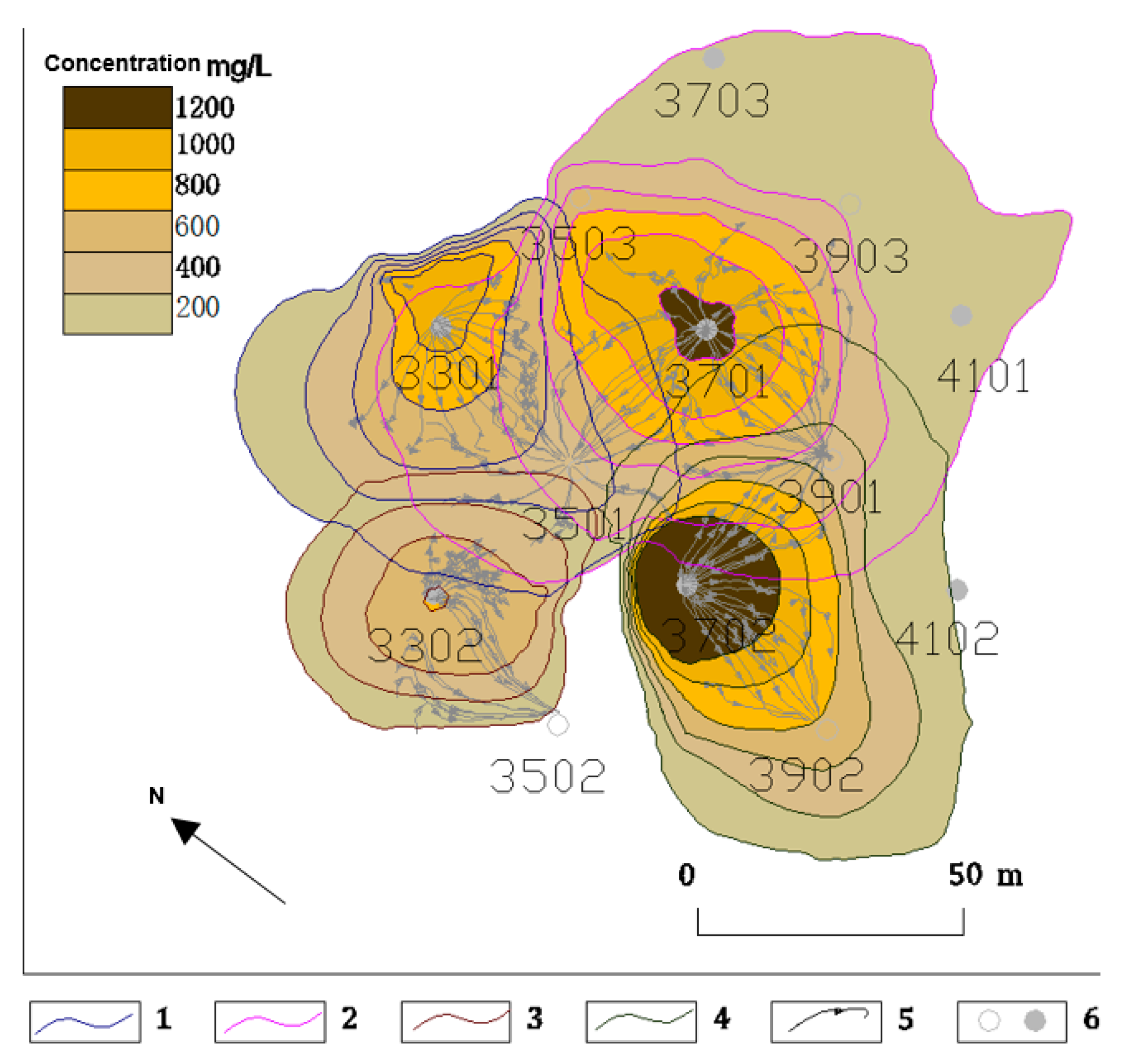
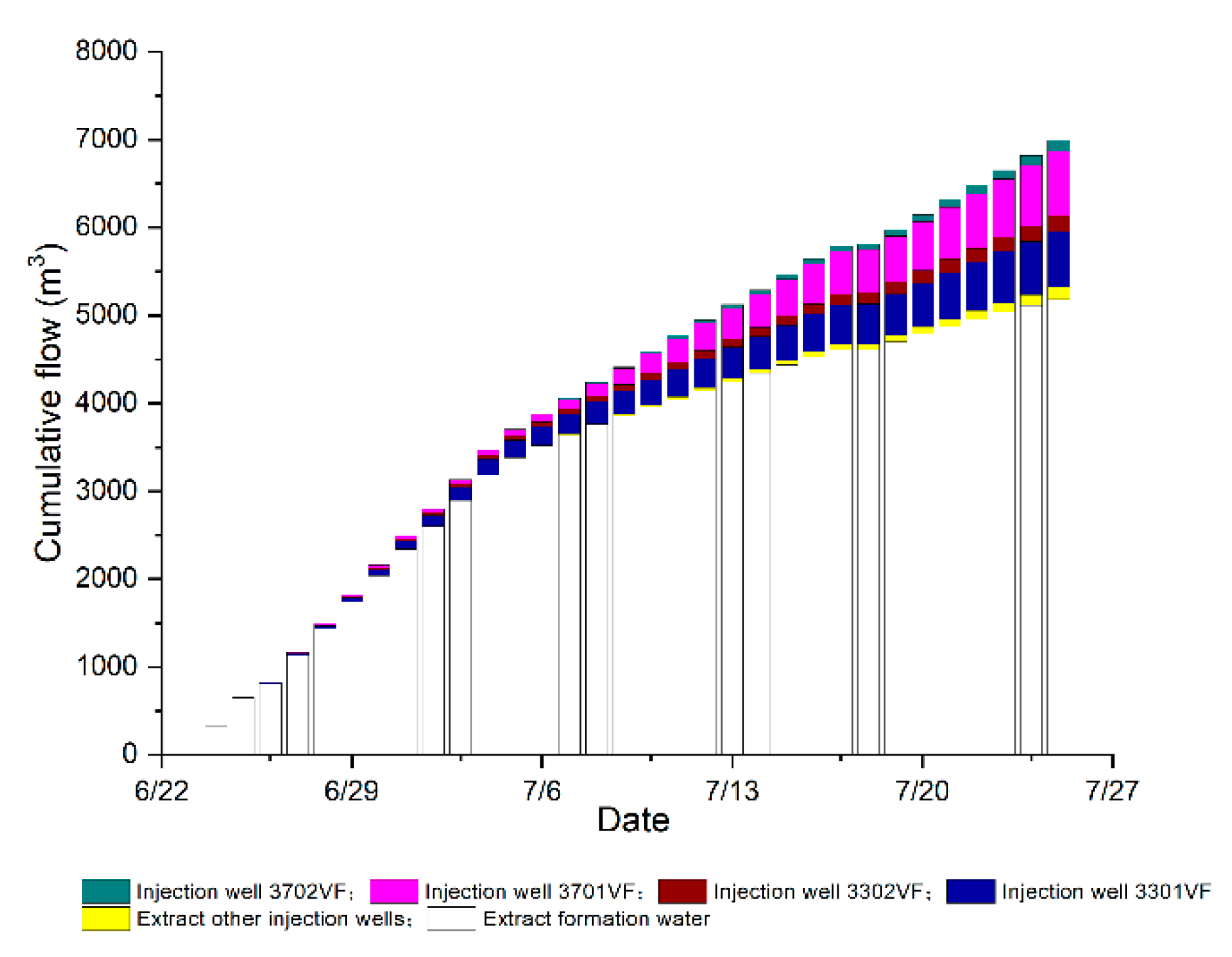
Aiming at the balance of pumping and injection flow in the ISL mining process, we proposed the concept of micro-balance of pumping and injection unit for the first time. Using the unit flow model as a means, through simulation, analysis, and calculation, we obtained the cumulative flow distribution of each pumping well and the solute flow direction of each injection well. On this basis, the unit flow is micro-balanced and adjusted to achieve the overall pumping balance of the stope finally.

(2)

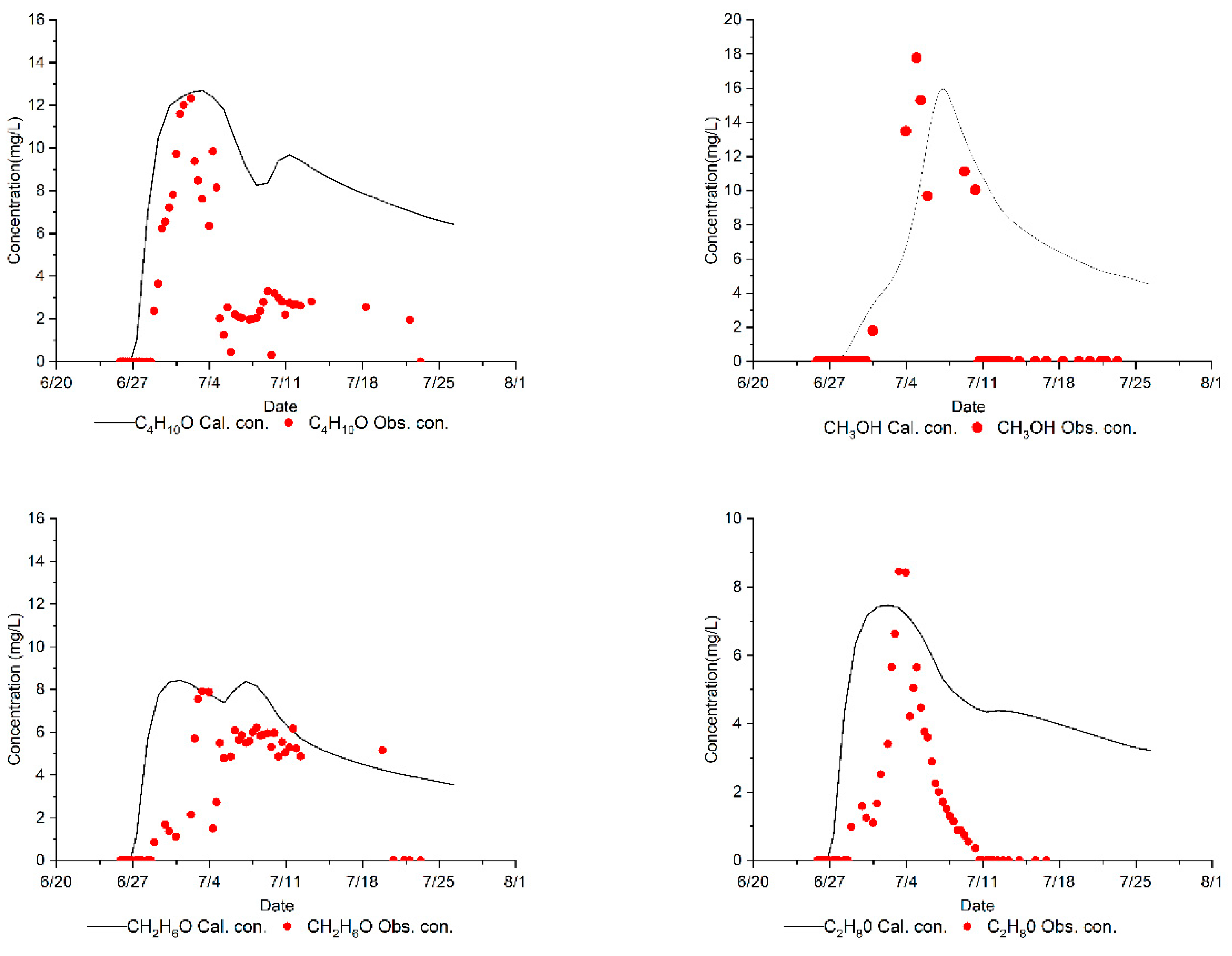
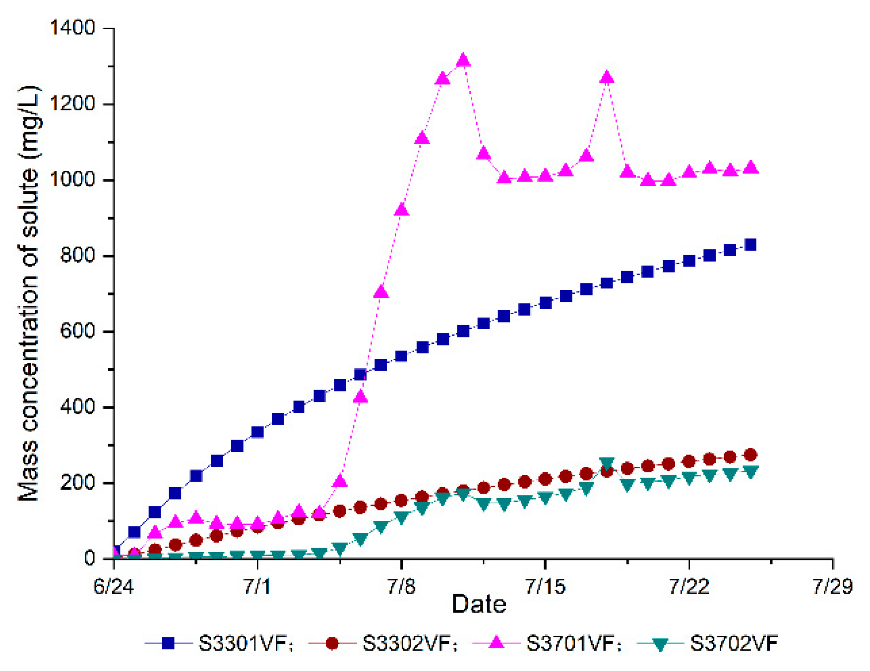
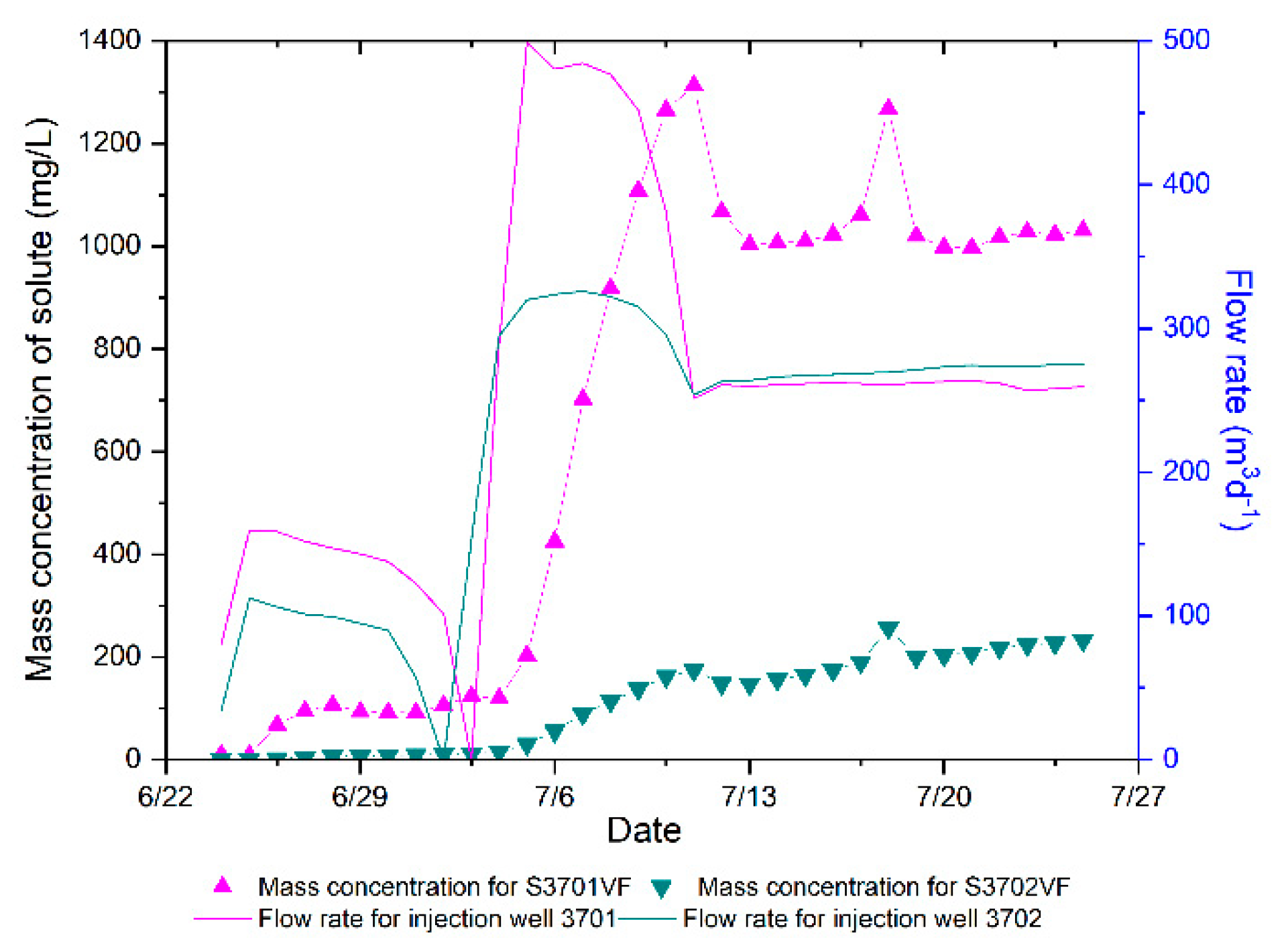
We established the calculation equation of the supply–demand flow rate of the pumping injection well in the extraction unit of the mining area. The tracer with unique directivity was used to trace the source of the well injection, and the ratio of the concentration of different tracers in the leachate was used to calculate the flow rate of different injection wells to the pumping wells. The two wells that account for the largest proportion of the extracted non-associated well flow, accounting for 1.1% and 0.8%, respectively, and the flow contribution distribution of the remaining injection wells were more evenly distributed.

(3)

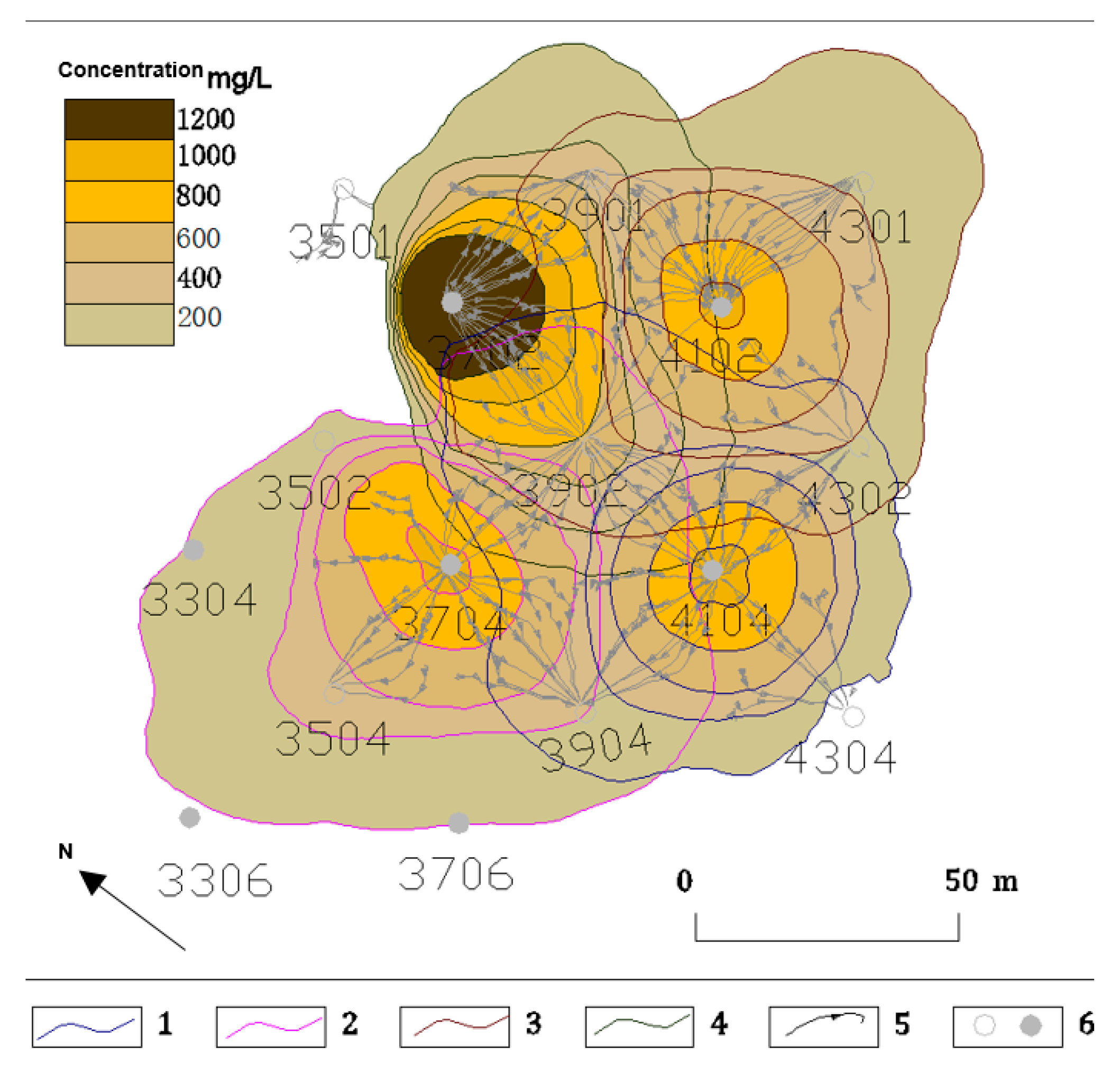
We established the flow micro-balance calculation and analysis process of the pumping and injection unit in the mining area. By completing the calculation and analysis of the flow balance of 72 boreholes in the entire mining area, we verified the analysis process. The simulation results showed that the application effect of the model was good, and the correlation coefficient of the solute transport model reached 0.8.

(4)

Through the above calculation and analysis, we laid out a solid theoretical and data basis for the micro-balance optimization of the flow rate of the extraction unit in the mining area. In the follow-up, the flow optimization of the pumping and injection unit in the mining area can be carried out in combination with the actual production conditions on-site, and the mining area can achieve uniform leaching.

(5)

In future work, the unit flow model verification of the mining area and the optimization of the flow micro-balance of the extraction unit of the mining area will be carried out.

References

1. Shang, D.; Geissler, B.; Mew, M.; Satalkina, L.; Zenk, L.; Tulsidas, H.; Haneklaus, N. Unconventional uranium in China’s phosphate rock: Review and outlook. Renew. Sustain. Energy Rev. 2021, 140, 110740. [Google Scholar] [CrossRef]
2. Sarangi, A.K.; Beri, K.K. Uranium mining by in-situ leaching. In Proceedings of the International Conference on “Technology management for Mining Processing and Environment”, Kharagpur, India, 1–3 December 2000. [Google Scholar]
3. Ma, Q.; Feng, Z.G.; Liu, P.; Lin, X.K.; Li, Z.G.; Chen, M.S. Uranium speciation and in situ leaching of a sand-stone-type deposit from China. J. Radioanal. Nucl. Chem. 2017, 311, 2129–2134. [Google Scholar] [CrossRef]
4. Su, X.B.; Du, Z.M. Development and prospect of China Uranium in-situ leaching technology. China Min. Mag. 2012, 21, 79–83. [Google Scholar]
5. Xie, T.T.; Ding, Y.; Zhou, G.M.; Xu, G.-L.; Li, H.-X.; Deng, J.X.; Zhang, C.; Xu, Z.-H. Numerical Simulation Analysis of Homologous Tracing Data Before and After Acidi-fication in the Conditional Experiment of an In-situ Leaching Uranium Mine. Uranium Min. Metall. 2018, 37, 1–8. [Google Scholar]
6. Wang, X.; Xie, T.; Yang, L.; Du, Z.; Wu, L.; Duan, B. Interwell tracer test in in-situ leaching uranium in one place of Xinjiang. Uranium Min. Metall. 2014, 33, 130–133. [Google Scholar]
7. Wang, H.; Guo, N.; Xie, Y.; Li, G. The influence of groundwater dilution on pregnant solution of in-situ leaching of uranium. Uranium Min. Metall. 2012, 31, 9–13. [Google Scholar]
8. Tweeton, D.R.; Peterson, K.A. Selection of lixiviants for in situ leach mining. In In Situ Mining Research; Information Circular; US Bureau of Mines: Washington, DC, USA, 1981; Volume 8852, pp. 17–24. [Google Scholar]
9. Roshal, A.; Kuznetsov, D. Simulation of propagation of leachate after the ISL mining closure. In Uranium in the Environment; Springer: Berlin/Heidelberg, Germany, 2006; pp. 217–224. [Google Scholar]
10. Bommer, P.M.; Schechter, R.S. Mathematical modeling of in-situ uranium leaching. Soc. Pet. Eng. J. 1979, 19, 393–400. [Google Scholar] [CrossRef]
11. Bernhard, G.; Geipel, G.; Brendler, V.; Nitsche, H. Uranium speciation in waters of different uranium mining areas. J. Alloy. Compd. 1998, 271, 201–205. [Google Scholar] [CrossRef]
12. Que, W.; Wang, H.; Yao, Y.; Tian, S.; Zhang, Z. Research status and development of in-situ leaching uranium techniques in China. Uranium Min. Metall. 2005, 24, 113–117. [Google Scholar]
13. Que, W.; Wang, H.; Niu, Y.; Gu, W.; Zhang, F. Development and prospect of china uranium mining and metallurgy. Eng. Sci. 2007, 5, 84–97. [Google Scholar]
14. Chen, J.; Liu, J. Study on sulphate and nitrate pollution in groundwater of a leaching uranium mine. In Proceedings of the 2012 2nd International Conference on Remote Sensing, Environment and Transportation Engineering, Nanjing, China, 1–3 June 2012; pp. 1–3. [Google Scholar]
15. Dangelmayr, M.A.; Reimus, P.W.; Johnson, R.H.; Clay, J.T.; Stone, J.J. Uncertainty and variability in laboratory derived sorption parameters of sediments from a uranium in situ recovery site. J. Contam. Hydrol. 2018, 213, 28–39. [Google Scholar] [CrossRef] [PubMed]
16. Sun, Y.Z.; Wu, A.X.; Li, J.H.; Zhao, G.Y. Mechanism and fluidity of solvents in in-situ leaching. Min. Res. Dev. 2001, 21, 1–3. [Google Scholar]
17. Zhao, C.H.; Li, G.M.; Lei, Q.F.; Ye, S.D. Numerical Simulation in A Test Field of In-Situ Leaching of Uranium. Geotech. Investig. Surv. 2008, 7, 27–31. [Google Scholar]
18. Yang, J.M.; Tan, K.X.; Huang, X.N. Evaluation and Analysis of Geologiacl Condition of In-Situ Fragmentation Leaching Uranium. China Nucl. Sci. Technol. Rep. 2003, 3. [Google Scholar] [CrossRef] [Green Version]
19. Zhao, L.; Deng, J.; Xu, Y.; Zhang, C. Mineral alteration and pore-plugging caused by acid in situ leaching: A case study of the Wuyier uranium deposit, Xinjiang, NW China. Arab. J. Geosci. 2018, 11, 1–11. [Google Scholar] [CrossRef]
20. Qi, H.; Tan, K.; Zeng, S.; Liu, J. Experimental study of in situ leaching uranium mining for low permeable sandstone uranium deposits using some surfactant. J. Nanhua Univ. Sci. Technol. 2010, 24, 19–23. [Google Scholar]
21. Zeng, Y.; Niu, Y.; Zhong, P.; Zhang, F. Overview of technical progresses in uranium mining and metallurgical industry in China. Uranium Min. Metall. 2003, 22, 24–28. [Google Scholar]
22. Wang, H.; Liu, N.; Su, X.; Liu, G.; Wu, W.; Tang, Q.; Wang, X. Alikaline in-situ leaching test of a uranium deposit in Xinjiang. Uranium Min. Metall. 2007, 26, 169–173. [Google Scholar]
23. Wang, H.F. The existing problems on in-situ leaching of uranium in China. Uranium Min. Metall. 2008, 27, 113–117. [Google Scholar]
Figure 1. Schematic diagram of the micro-balance calculation principle of the injection unit.
Processes 09 01288 g001
Figure 2. Flow chart of micro-balance calculation for flow rate of pumping and injection unit in mining area.
Processes 09 01288 g002
Figure 3. Statographic view of the Saihan Formation. (Note: 1—irdingmanha group; 2—upper part of Saihan group; 3—lower section of Saihan group; 4—lithological boundary; 5—parallel unconformity; 6—angle unconformity; 7—oxidation zone; 8—gray sandstone; 9—regional aquifers; 10—local aquifers; 11—uranium ore body; 12—uranium mineralized body).
Processes 09 01288 g003
Figure 4. Flow chart of micro-balance calculation for flow rate of pumping and injection unit in mining area. (Note: 1—mining area; 2—boundary of area model; 3-research area; 4—boundary of solute transport model; 5—scope of simulated drilling).
Processes 09 01288 g004
Figure 5. Schematic diagram of injection well for flow adjustment in target mining area.
Processes 09 01288 g005
Figure 6. Flow regulation curve of 3308 injection well at the edge of mining area.
Processes 09 01288 g006
Figure 7. Distribution of polyol tracer and solute monitoring points.
Processes 09 01288 g007
Figure 8. Time dependence curves of observed and calculated concentrations of four alcohol tracers in leaching solution of central monitoring well.
Processes 09 01288 g008
Figure 9. Schematic diagram of neutral solute number and corresponding injection well in the model.
Processes 09 01288 g009
Figure 10. Solute migration distribution of unit 3501 on Day 32. (Note: 1—migration range of solute S3301; 2—migration range of solute S3701; 3—migration range of solute S3302; 4—migration range of solute S3702; 5—flow field streamlines of ISL of uranium; 6—pumping and injection wells in the stope).
Processes 09 01288 g010
Figure 11. Mass change chart of solute concentration in unit 3501.
Processes 09 01288 g011
Figure 12. Injection flow and corresponding solute concentration.
Processes 09 01288 g012
Figure 13. Solute composition analysis diagram of pumping well 3501.
Processes 09 01288 g013
Figure 14. Solute migration distribution of unit 3902 on day 32. (Note: 1—migration range of solute S4104; 2—migration range of solute S3704; 3—migration range of solute S4102; 4—migration range of solute S3702; 5—flow field streamlines of ISL of uranium; 6—pumping and injection wells in the stope).
Processes 09 01288 g014
Figure 15. Mass change chart of solute concentration in unit 3902.
Processes 09 01288 g015
Figure 16. Solute composition analysis diagram of pumping well 3902.
Processes 09 01288 g016