Magnetic Dipole and Thermal Radiation Impacts on Stagnation Point Flow of Micropolar Based Nanofluids over a Vertically Stretching Sheet: Finite Element Approach

Abstract

An analysis for magnetic dipole with stagnation point flow of micropolar nanofluids is modeled for numerical computation subject to thermophoresis, multi buoyancy, injection/suction, and thermal radiation. The partial derivative is involved in physical consideration, which is transformed to format of ordinary differential form with the aid of similarity functions. The variational finite element procedure is harnessed and coded in Matlab script to obtain the numerical solution of the coupled non-linear ordinary differential problem. The fluid temperature, velocity, tiny particles concentration, and vector of micromotion are studied for two case of buoyancy (assisting $0<\lambda$, and opposing $0>\lambda$) through finite-element scheme. The velocity shows decline against the rising of ferromagnetic interaction parameter $\left(\beta \right)$ (assisting $0<\lambda$ and opposing $0>\lambda$), while the inverse behaviour is noted in micro rotation profile. Growing the thermo-phoresis and microrotation parameters receded the rate of heat transfer remarkable, and micromotion and fluid velocity enhance directly against buoyancy ratio. Additionally, the rate of couple stress increased against rising of thermal buoyancy $\left(\lambda \right)$ and boundary concentration $\left(m\right)$ in assisting case, but opposing case shows inverse behavior. The finite element scheme convergency was tested by changing the mesh size, and also test the validity with available literature.

1. Introduction

Ferrofluids are the suspension of nanoscale ferromagnetic particles in fluid carrier and magnetized by the influence of magnetic field [1]. In recent years, the investigation on ferromagnetic fluids (FF) has also become interested due to wide application in the field of chemical engineering, bio-medicine, nuclear power plants, robotics, compounds, micro-electro-mechanical, melted metals refinement, pumps, colored stains, X-ray machine, and shock absorbers, etc. [2,3]. In 1965, Stephen [4] pioneered the concept of ferrofluids (FF). This type of hybrid fluids is actually, a suspension of colloidal ferromagnetic particles (10 nm) in a base liquid. In the presence of a magnetic field, these fluids exhibit magnetization to avoid their possible settling. In medical sciences, pain relief is managed with magnet therapy. Electromechanical devices such as recording procedures and generators are associated with magnet interactions. Furthermore, these fluids are used in enhancing the heat transfer rate. The study of ferromagnetic impacts in a liquid metal was initially considered by Albrecht et al. [5]. Anderson and Valnes [6] presented fundamentals of ferromagnetic fluid flow. Shliomis [7] established the basic analytical models concerning to the motion of ferrofluids. Neuringer and Rosensweig [8] developed a formulation for the impact of magnetic body force with a consideration that the magnetic field is parallel to magnetization. Magnetization being temperature dependent, such a thermomagnetic coupling may result in various practical applications of ferrofluids (see [9]).

Fluids with microstructures are micropolar fluids [10]. Stiff randomly oriented particles make up micropolar fluids. Some physical specimens of micropolar flow are liquid crystals, blood flow, bubby liquids. The basic concepts of micropolar fluid, with some applications in engineering, was firstly described in (1966) by Eringen [11]. From recent decades, the interest of researchers in the theory of micropolar fluids have a significantly enlarged cause of its immense applications in industrial and engineering fields such as polymeric and colloids deferments, liquid crystal, liquid minerals, body fluids, engine lubricants, paint rheology, cervical flow, and thrust bearing technology [12,13]. The steady micropolar based fluid passed through impermeable and permeable sheets was investigated by Hassanien et al. [14]. The heat transfer of micropolar fluid flow was studied by Turkyilmazoglu [15]. The multi slips effects on dynamics of magnetohydrodynamic micropolar based tiny particles suject to heat source were investigated by Sohaib et al. [16].

Several analysts have considered a continuously extending surface to study of boundary layer flow in recent decades because of its numerous applications in engineering and industry [17,18]. Some applications are: paper production, metal-spinning, crystal sheets productions, drawing of plastic films, polymer dispensation of chemical engineering plants, and coating of cable, etc. Crane’s [19] groundbreaking work examined the steady flow through the linearly stretching plate. To study the influence of viscous and suction, Faraz et al. [20] examined the an axisymmetric geometry flow on the shrinking surface. The effects of injection/suction subject to mass and heat transfer over an extending sheet were discussed in Gupta [21]. The point on the surface of object in the field of flow where the fluid is brought at rest by the object is called stagnation point. The magneto hydrodynamics stagnation point flows with heat transfer effects are important in both practice and theory. Some practical applications include liquid crystals, blood flow, the aerodynamics extrusion of plastic sheets, the cooling of an infinite metallic plate in a cooling bath and textile and paper industries [22,23]. Many researchers have deliberated the stagnation point flow over a stretching sheet [24,25]. Chiam [26] studied a two-dimensional stagnation point flow of viscous fluid over a linearly stretching surface. Amjad et al. [27] examined the Casson micropolar based tiny particles flow in the stagnation point zone over a curved surface.

A designed fluid that can be utilized in the advanced technological areas with enormous diffusivity heat capacity is called nanofluid. Nanotechnology has recently piqued the interest of many scientists due to its widespread use in industry as a result of nano-sized particles possessing a wide range of chemical and physical properties [28,29]. The tiny particles made by nanomaterials are generally utilized as a coolant in mechanical, industrial, and chemical fields [30], and are utilized in various assembling applications, for example, cooking handling, cool, vehicle radiators, waste heat recovery, refrigeration, and so forth [31]. To begin, Choi [32] introduced the nanofluid in 1995, and he introduce a fluid with tiny particles whose size less than (100nm) diameter. Vehicle cooling, fuel cells, lubricants, heat exchangers, cancer therapy, and micro-electro-mechanical structures are just a few of the applications for heat transfer and nanofluid boundary layer flow in science and engineering [33,34]. As a result, many researchers have experimented with and analyzed the flow and heat transfer physiognomies of nanofluids. Unsteady boundary layer flow of nanofluids through a penetrable shrinking/stretching sheet was observed by Bachok et al. [35]. Wen [36] speaks to the lacking minding of the structure and component of nanofluids and furthermore their applications. The brownian motion of tiny particles enhanced the host fluid heat transfer rate reported by Rasheed et el. [37] and Ali et al. [38]. More work on nanofluid subject to various types of flow geometry is carried out [39,40,41].

The first aim of the current examination is to research the conduct of magnetic dipole along with the stagnation point flow of micropolar based nanofluid over a vertical stretching surface. Because of the complexity of technological processes, a quest for enhance base fluid thermal efficacy is the rising research zone. The model of nanofluid has created enough capacity to meet the growing demands. The majority of previous studies used simple fluids (water base fluid), but there exist non-Newtonian fluid that are more viscous in practice. The conduct of the involved parameters is exhibited graphically by a precise discussion. Besides, the graphical portrayal of the Nusselt number, skin friction coefficient, and the Sherwood number coefficient is discussed. Furthermore, with Matlab coding, the most powerful finite element based computation carried out, and also test the accuracy and convergence of finite element scheme.

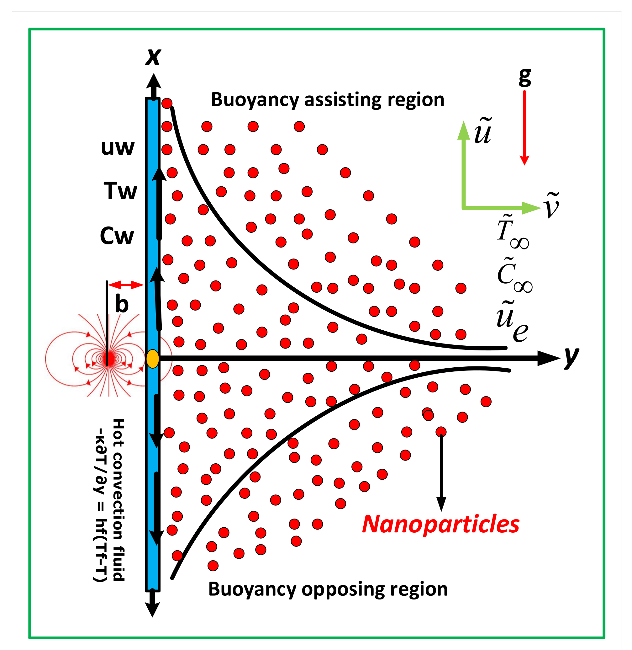
2. Mathematical Formulation (Magnetization+)

Consider two dimensional, steady, and incompressible flow acceleration because of a vertical positioned surface, and fluid is contemplated across $0<y$ there in pictographic depiction Figure 1 in allusion to the OXY-Coordinate system. We presumed a stagnation-point flow of 2-D incompressible micropolar nanofluid across the surface. The surface is presumed to be stretched with velocity ${\tilde{U}}_w=\tilde{a}x$ and ${\tilde{u}}_e\left(x\right)=\tilde{c}x$ (external flow or free stream) is the flow rate away from the boundary layer and is assumed to be the hot fluid along side the $-{\kappa }_f\left(\frac{\partial \tilde{T}}{\partial y}\right)=h_f({\tilde{T}}_f-\tilde{T})$ vertical wall. The magnet dipole is centered outside the liquid at a distance b, with its core at (0,b) on the y-axis and the magnet field pointing along the positive x-axis. It is stated that, $\tilde{T}$ is the temperature of fluid, and $\widetilde{Tc}$ is a curie temperature often more appropriate as compared to $\widetilde{T_w}$ (wall surface temperature), whereas the acoustic fluid temperature far from the sheet is ${\tilde{T}}_{\infty }=\widetilde{Tc}$, but there is no more magnetic flux there until the magnetic nanofluid exceeds to Curie temperature $\widetilde{Tc}$. The condensed structure of the system of equations has predicated from the above assumptions having boundary layer evaluations are (see [42,43]):

$$\begin{array}{c}\frac{\partial \tilde{u}}{\partial x}+\frac{\partial \tilde{v}}{\partial y}=0,\\ \tilde{u}\frac{\partial \tilde{u}}{\partial x}+\tilde{v}\frac{\partial \tilde{u}}{\partial y}={\tilde{u}}_e\frac{\partial {\tilde{u}}_e}{\partial x}+\frac{{\mu }_0}{\rho }M\frac{\partial \tilde{H}}{\partial x}+\left(\frac{{\mu }_f+\kappa }{{\rho }_f}\right)\frac{{\partial }^2\tilde{u}}{\partial y^2}+\frac{\kappa }{{\rho }_f}\frac{\partial \tilde{w}}{\partial y}\end{array}$$

(1)

$$\begin{array}{c}+\frac{g}{{\rho }_f}\left[{\rho }_f{\beta }_t(\tilde{T}-{\tilde{T}}_{\infty })(1-{\tilde{C}}_{\infty })+{\beta }_c({\rho }_p-{\rho }_{f_{\infty }})(\tilde{C}-{\tilde{C}}_{\infty })\right],\end{array}$$

(2)

$$\begin{array}{c}\tilde{u}\frac{\partial \tilde{w}}{\partial x}+\tilde{v}\frac{\partial \tilde{w}}{\partial y}=\frac{{\gamma }_f}{\left({\rho }_f\right)j}\frac{{\partial }^2\tilde{w}}{\partial y^2}-\frac{\kappa }{\left({\rho }_f\right)j}(2\tilde{w}+\frac{\partial \tilde{u}}{\partial y}),\end{array}$$

(3)

$$\begin{array}{c}\tilde{u}\frac{\partial \tilde{T}}{\partial x}+\tilde{v}\frac{\partial \tilde{T}}{\partial y}+\left(\tilde{u}\frac{\partial {\tilde{H}}^{*}}{\partial x}+\tilde{v}\frac{\partial {\tilde{H}}^{*}}{\partial y}\right){\mu }_0\tilde{T}\frac{\partial \tilde{M}}{\partial \tilde{T}}=\tilde{\alpha }\frac{{\partial }^2\tilde{T}}{\partial y^2}-\frac{\partial {\tilde{q}}_r}{\partial y}+\tilde{\tau }\left(\frac{D_T}{{\tilde{T}}_{\infty }}{\left(\frac{\partial \tilde{T}}{\partial y}\right)}^2+{\tilde{D}}_B\frac{\partial \tilde{T}}{\partial y}\frac{\partial \tilde{C}}{\partial y}\right),\end{array}$$

(4)

$$\begin{array}{c}\tilde{u}\frac{\partial \tilde{C}}{\partial x}+\tilde{v}\frac{\partial \tilde{C}}{\partial y}=D_s\frac{{\partial }^2\tilde{C}}{\partial y^2}+\frac{D_T}{{\tilde{T}}_{\infty }}\left(\frac{{\partial }^2\tilde{T}}{\partial y^2}\right).\end{array}$$

(5)

where, $\tilde{u},\tilde{v}$ are the velocity components in x, y directions, respectively, $\tilde{C}$, $\tilde{T}$ are the tiny particles’ volume concentration and fluid temperature, respectively, ${\tilde{D}}_B$, ${\tilde{D}}_T$, $g^{*}$, ${\beta }_T$, ${\beta }_c$, and are the Brownian diffusion, thermophoretic diffusion coefficient, gravitational acceleration, the thermal, and nanoparticle volume concentration expansion coefficient, respectively. ${\tilde{\tau }}^{*}={\left(\rho c\right)}_p{\left(\rho c\right)}_f$ is the ratio of the nanoparticle material’s effective heat capacity to the heat capacity of the fluid. The spin gradient viscosity $\gamma =(\mu j+\frac{\kappa }{2}j)={\mu }_f(j+\frac{K}{2}j)$ was assumed by Khan et al. [44], where the material parameter is denoted by $K=\frac{\kappa }{\mu }$ In addition, the intensity of the fluid is $\rho$, thermal diffusion $\tilde{\alpha }$, viscosity $\kappa$, micro-inertia j, and $\tilde{\omega }$ is the angular velocity, respectively. The radiation heat flux is defined below [45]:

$${\tilde{q}}_r=\frac{4}{3}\frac{{\alpha }^{*}}{K_1}\frac{\partial {\tilde{T}}^4}{\partial y^2}$$

The Roseland mean coefficient of absorption is $K_1$, whereas the Stefan Boltzman constant is ${\alpha }^{*}$. Slight temperature variations in a flow are taken into consideration, and thus the Taylor series has been used to neglect higher-order terms; the result is

$$\frac{\partial {\tilde{q}}_r}{\partial y}=\frac{-16{\alpha }^{*}{\tilde{T}}_{\infty }^3}{3K_1}\frac{{\partial }^2\tilde{T}}{\partial y^2}$$

The respective boundary parameters of the preceding problem are

$$\begin{array}{c}\tilde{u}-{\tilde{U}}_w\left(x\right)=\tilde{a}x,\tilde{v}-{\tilde{v}}_w=0,\tilde{\omega }=-m\frac{\partial u}{\partial y},{\kappa }_f\left(\frac{\partial \tilde{T}}{\partial y}\right)=(h_f{\tilde{T}}_{\tilde{f}}-h_f\tilde{T}),\tilde{C}={\tilde{C}}_w\left(x\right),asy=0,\end{array}$$

(6)

$$\begin{array}{c}\tilde{u}\to {\tilde{u}}_e=\tilde{c}x,\tilde{\omega }\to 0,\tilde{T}\to {\tilde{T}}_{\infty },\tilde{C}\to {\tilde{C}}_{\infty },asy\to \infty .\end{array}$$

(7)

where ${\tilde{T}}_f$ denotes temperature and ${\tilde{C}}_w$ represents the nano-particle’s concentration at the surface. ${\tilde{T}}_{\infty }$ and ${\tilde{C}}_{\infty }$ are the corresponding ambient values. The m parameter is a boundary constant parameter with a value of $0\le m\le 1$. As $m=0$, the microelements cannot rotate, $\tilde{\omega }=0$ takes place on the surface, $0.5=m$ correlates the antisymmetric components of stress tensor vanishing, and $1.0=m$ coincides turbulent flow of boundary layer. The progression of magnetic ferrofluid is influenced by the magnetic field, because the magnetic dipole with magnetic scalar potential is denoted as (see [46,47]):

$$\Psi =\frac{{\gamma }^{*}}{2\tilde{\pi }}\left(\frac{x}{x^2+{(y+b)}^2}\right)$$

(8)

After that, ${\gamma }^{*}$ stand for strength of magnetic field, and magnetic field amplitudes besides the x and y-axis are written as:

$$\begin{array}{c}{\tilde{H}}_x^{*}=-\frac{\partial \Psi }{\partial x}=\frac{{\gamma }^{*}}{2\tilde{\pi }}\left\{\left(\frac{x^2-(y^2+b^2+2yb)}{{(x^2+{(y+b)}^2)}^2}\right)\right\},\end{array}$$

(9)

$$\begin{array}{c}{\tilde{H}}_y^{*}=-\frac{\partial \Psi }{\partial y}=\frac{{\gamma }^{*}}{2\tilde{\pi }}\left\{\left(\frac{2xy+2xb)}{{(x^2+{(y+b)}^2)}^2}\right)\right\}.\end{array}$$

(10)

Since the magnetic force is proportional to the slope of $\tilde{H}$. The corresponding magnitude H of the magnetic field strength is described as follows

$$\begin{array}{c}{\tilde{H}}^{*}={\left[{\left(\frac{\partial \Psi }{\partial x}\right)}^2+{\left(\frac{\partial \Psi }{\partial y}\right)}^2\right]}^{\frac{1}{2}},\end{array}$$

(11)

$$\begin{array}{c}\frac{\partial {\tilde{H}}^{*}}{\partial x}=-\left(\frac{2x}{{(y+b)}^4}\right)\frac{{\gamma }^{*}}{2\tilde{\pi }},\end{array}$$

(12)

$$\begin{array}{c}\frac{\partial {\tilde{H}}^{*}}{\partial y}=-\left(\frac{-2}{{(y+b)}^3}+\frac{4x^2}{{(y+b)}^5}\right)\frac{{\gamma }^{*}}{2\tilde{\pi }}.\end{array}$$

(13)

The conversion of M into magnetization can be assumed temperature as a linear function.

$$M=(T_c-\tilde{T}){\beta }^{*}$$

(14)

for which ${\beta }^{*}$ represent the pyromagnetic coefficient constant. In whichever case, the following point is critical for the ferrohydrodynamic partnership event: (i) the temperature of fluid $\tilde{T}$ is specific in comparison to the external magnetic field $\widetilde{T_C}$, and (ii) the external magnetic field is different from the bulk. Further, no need to magnetization, once obtained the $T_C$. The physical universality is important in view of the extremely high Curie temperature of iron, which is 1043 K. The following similarity transforms are used to convert Equations (1)–(5) to ordinary differential form (see [48,49]):

$$\begin{array}{c}\left.\begin{array}{c}\hfill \psi (\eta ,\xi )=\left(\frac{\mu }{\rho }\right)\eta f\left(\xi \right),\theta (\eta ,\xi )=\frac{T_c-T}{T_c-T_w},\eta =\sqrt{\frac{c\mu }{\rho }}x,\xi =\sqrt{\frac{c\mu }{\rho }}y,\\ \hfill \tilde{u}=\frac{\partial \psi }{\partial x}=\tilde{a}x{f}^{\prime }\left(\xi \right),\tilde{v}=-\frac{\partial \psi }{\partial y}=-\sqrt{\tilde{a}\nu }f\left(\xi \right),g=\frac{\tilde{\omega }}{\tilde{a}x}\sqrt{\frac{\nu }{\tilde{a}}}.\end{array}\right\}\end{array}$$

(15)

The stream function, and dimensionless coordinates are represented by $\psi$, $\eta$, and $\xi$, respectively. Equations (2)–(7) are transformed into ODE’s using Equation (15)

$$\begin{array}{c}(K+1)\frac{d^{3}f}{d{\xi }^3}-{\left(\frac{df}{d\xi }\right)}^2+f\frac{d^{2}f}{d{\xi }^2}+K\frac{dg}{d\xi }-\frac{2\beta {\theta }_1}{{(\xi +\gamma )}^4}\pm \lambda \left(\theta +Nr\varphi \right)+R^2=0,\end{array}$$

(16)

$$\begin{array}{c}(1+\frac{K}{2})\frac{d^{2}g}{d{\xi }^2}+f\frac{dg}{d\xi }-g\frac{df}{d\xi }-K\left(2g+\frac{d^{2}f}{d{\xi }^2}\right)=0,\end{array}$$

(17)

$$\begin{array}{c}\frac{1}{Pr}(1+Rd)\frac{d^2\theta }{d{\xi }^2}+f\frac{d\theta }{d\xi }+Nb\frac{d\theta }{d\xi }\frac{d\varphi }{d\xi }+Nt{\left(\frac{d\theta }{d\xi }\right)}^2+\frac{2{\lambda }_1\beta ({\theta }_1-ϵ)f}{Pr{(\xi +\gamma )}^3}=0,\end{array}$$

(18)

$$\begin{array}{c}\frac{d^2\varphi }{d{\xi }^2}+Lef\frac{d\varphi }{d\xi }+\frac{Nb}{Nt}\frac{d\theta }{d\xi }=0,\end{array}$$

(19)

$$\begin{array}{c}\left.\begin{array}{c}\hfill f\left(\xi \right)=f_w,\frac{df}{d\xi }=1,g\left(\xi \right)=-m\frac{d^{2}f}{d{\xi }^2},\frac{d\theta }{d\xi }-C\theta \left(\xi \right)=-C,\varphi \left(\xi \right)=1,at\xi =0,\\ \hfill \frac{df}{d\xi }\to R,g\to 0,\theta \left(\xi \right)\to 0,\varphi \left(\xi \right)\to 0,as\xi \to \infty .\end{array}\right\}\end{array}$$

(20)

The developing parameters in Equations (16)–(20) are defined as

$$\begin{array}{c}K=\frac{\kappa }{\mu },Pr=\frac{\nu }{\tilde{\alpha }},Le=\frac{\nu }{{\tilde{D}}_B},R_d=\frac{16{\sigma }^{*}{\tilde{T}}_{\infty }^3}{3k^{*}K},Nb=(\tau {\tilde{D}}_B{\tilde{C}}_w-\tau {\tilde{D}}_B{\tilde{C}}_{\infty }){\nu }^{-1},Nt=\frac{\tau {\tilde{D}}_T({\tilde{T}}_w-{\tilde{T}}_{\infty }){\nu }^{-1}}{{\tilde{T}}_{\infty }},\\ R^2=\frac{{\tilde{c}}^2}{{\tilde{a}}^2},f_w=-\frac{v_w}{\sqrt{\tilde{a}\nu }},C=-\frac{h_f}{{\kappa }_f}\sqrt{\frac{\nu }{\tilde{a}}},G_{rt}=\frac{g{\rho }_{f\infty }{\beta }_t(1-{\tilde{C}}_{\infty })({\tilde{T}}_w-{\tilde{T}}_{\infty })x^3}{{\nu }^2},R{a}_x=\frac{{\tilde{U}}_w\left(x\right)x}{\nu },\\ G_{rc}=\frac{g{\beta }_c({\rho }_p-{\rho }_{f\infty })({\tilde{C}}_w-{\tilde{C}}_{\infty })x^3}{{\nu }^2},Nr=\frac{{\beta }_c({\rho }_p-{\rho }_{f\infty })({\tilde{C}}_w-{\tilde{C}}_{\infty })}{{\beta }_t{\rho }_f(1-{\tilde{C}}_{\infty })({\tilde{T}}_w-{\tilde{T}}_{\infty })},\lambda =\frac{G_{rt}}{R{a}_x^2},{\lambda }_1=\frac{c{\mu }^2}{\rho k(T_c-T_w)},\\ \beta =\frac{{\gamma }^{*}\rho {\mu }_0}{2\pi {\mu }^2}k(T_c-T_w),\gamma =d\sqrt{\frac{c\rho }{\mu }},\end{array}$$

and $ϵ=\frac{T_c}{(T_c-T_w)}$ symbolizes a material’s parameter (K), Lewis number ($Le$), radiation parameter ($Rd$), thermophoresis parameter ($Nt$), Prandtl number ($Pr$), Brownian motion parameter ($Nb$), here $R^2$ is the constant, suction/injection parameter ($f_w$), and Biot (C), thermal Grashof ($G_{rt}$), solutal Grashof ($G_{rc}$), local Renolds ($R{a}_x$), Eckert (${\lambda }_1$) numbers. Moreover buoyancy ratio ($Nr$), mixed convection ($\lambda$), ferrohydrodynamic interaction ($\beta$) parameters, dimensionless distance($\gamma$), and Curie temperature ratio ($ϵ$). Further to that, a similar intensity of unity is applied to both buoyancy and thermal forces, regarding the positive values for cumulative buoyancy forces resulting in negative attributes and supporting flow resulting in competing for flow.

The terms for skin friction coefficient, Nusselt number, and the Sherwood number are as follows

$$\begin{array}{c}{\tilde{C}}_f=\frac{{\tau }_w}{\rho {\widetilde{U^2}}_{w}2},Nu=\frac{x{q}_w}{\kappa ({\tilde{T}}_w-{\tilde{T}}_{\infty })},Shr=\frac{x{q}_m}{{\tilde{D}}_B({\tilde{C}}_w-{\tilde{C}}_{\infty })}.\end{array}$$

(21)

From which the skin friction tensor at the wall is ${\tau }_w={\left[\kappa \omega +(\mu +\kappa )\frac{\partial \tilde{u}}{\partial y}\right]}_{y=0}$, at the wall, the heat fluxion is $q_w={\left[(\kappa +\frac{16\alpha {\tilde{T}}^3}{3\kappa })\frac{\partial \tilde{T}}{\partial y}\right]}_{y=0}$, and the fluxion of mass from the surface $q_m={\left({\tilde{D}}_B\frac{\partial \tilde{C}}{\partial y}\right)}_{y=0}$. With the help of Equation (10), the following can be obtained

$$\left\{\begin{array}{c}\hfill \frac{1}{2}{\tilde{C}}_f{R{e}_x}^2=(1+(1-m)K)f^{\prime \prime }\left(0\right),\\ \hfill {R{e}_x}^{\frac{-1}{2}}Nu=-(Rd+1){\theta }^{\prime }\left(0\right),\\ \hfill {R{e}_x}^{\frac{-1}{2}}Shr=-{\varphi }^{\prime }\left(0\right).\end{array}\right.$$

(22)

3. Numerical Procedure

The finite-element technique is notable to address different kinds of differential equation. This technique include continuous piecewise approximation, which minimize the size of error [50]. The crucial steps and an extraordinary portrayal of this strategy sketched out by jyothi [51] and Reddy [52]. This technique is very productive tool described by the experts and scientists to examine the complicated problems of engineering because of its simplicity and accuracy [53,54,55]. To solve the Equations (16)–(19) along boundary Condition (20), we first consider:

$$\begin{array}{c}\frac{df}{d\xi }=h,\end{array}$$

(23)

Using Equation (23), Equations (16)–(20) are converted to (24) to (28), and are given as

$$\begin{array}{c}(K+1)\frac{d^{2}h}{d{\xi }^2}+f\frac{dh}{d\xi }-h^2+K\frac{dg}{d\xi }-\frac{2\beta {\theta }_1}{{(\xi +\gamma )}^4}\pm \lambda \left(\theta +Nr\varphi \right)+R^2=0,\end{array}$$

(24)

$$\begin{array}{c}(1+\frac{K}{2})\frac{d^{2}g}{d{\xi }^2}+f\frac{dg}{d\xi }-gh-K\left(2g+\frac{dh}{d\xi }\right)=0,\end{array}$$

(25)

$$\begin{array}{c}\frac{1}{Pr}(1+Rd)\frac{d^2\theta }{d{\xi }^2}+f\frac{d\theta }{d\xi }+Nb\frac{d\theta }{d\xi }\frac{d\varphi }{d\xi }+Nt{\left(\frac{d\theta }{d\xi }\right)}^2+\frac{2{\lambda }_1\beta ({\theta }_1-ϵ)f}{Pr{(\xi +\gamma )}^3}=0,\end{array}$$

(26)

$$\begin{array}{c}\frac{d^2\varphi }{d{\xi }^2}+Lef\frac{d\varphi }{d\xi }+\frac{Nb}{Nt}\frac{d\theta }{d\xi }=0,\end{array}$$

(27)

$$\begin{array}{c}\left.\begin{array}{c}\hfill h\left(\xi \right)=1,f\left(\xi \right)-f_w=0,g\left(\xi \right)+\left(m\right)\frac{dh}{d\xi }=0,\varphi \left(\xi \right)=1.0,\frac{d\theta }{d\xi }=-(C+C\theta \left(\xi \right)),at\xi =0.0,\\ \hfill h\to R,g\to 0.0,\theta \left(\xi \right)\to 0.0,\varphi \left(\xi \right)\to 0.0,as\xi \to \infty .\end{array}\right\}\end{array}$$

(28)

The variational forms of Equations (23)–(27) subject to linear-element ${\Omega }_{\xi }=({\xi }_{\tilde{a}},{\xi }_{\tilde{a}+1})$ are given below

$$\begin{array}{c}{\int }_{{\xi }_{\tilde{a}}}^{{\xi }_{\tilde{a}+1}}\widetilde{w_1}\{\frac{df}{d\xi }-h\}d\xi =0,\end{array}$$

(29)

$$\begin{array}{c}{\int }_{{\xi }_{\tilde{a}}}^{{\xi }_{\tilde{a}+1}}\widetilde{w_2}\left\{(K+1)\frac{d^{2}h}{d{\xi }^2}+f\frac{dh}{d\xi }-h^2+K\frac{dg}{d\xi }-\frac{2\beta {\theta }_1}{{(\xi +\gamma )}^4}\pm \lambda \left(\theta +Nr\varphi +Rb\gamma \right)+R^2\right\}d\xi =0,\end{array}$$

(30)

$$\begin{array}{c}{\int }_{{\xi }_{\tilde{a}}}^{{\xi }_{\tilde{a}+1}}\widetilde{w_3}\left\{(1+\frac{K}{2})\frac{d^{2}g}{d{\xi }^2}+f\frac{dg}{d\xi }-gh-K\left(2g+\frac{dh}{d\xi }\right)\right\}d\xi =0,\end{array}$$

(31)

$$\begin{array}{c}{\int }_{{\xi }_{\tilde{a}}}^{{\xi }_{\tilde{a}+1}}\widetilde{w_4}\left\{\frac{1}{Pr}(1+Rd)\frac{d^2\theta }{d{\xi }^2}+f\frac{d\theta }{d\xi }+Nb\frac{d\theta }{d\xi }\frac{d\varphi }{d\xi }+Nt{\left(\frac{d\theta }{d\xi }\right)}^2+\frac{2{\lambda }_1\beta ({\theta }_1-ϵ)f}{Pr{(\xi +\gamma )}^3}\right\}d\xi =0,\end{array}$$

(32)

$$\begin{array}{c}{\int }_{{\xi }_{\tilde{a}}}^{{\xi }_{\tilde{a}+1}}\widetilde{w_5}\left\{\frac{d^2\varphi }{d{\xi }^2}+Lef\frac{d\varphi }{d\xi }+\frac{Nb}{Nt}\frac{d\theta }{d\xi }\right\}d\xi =0.\end{array}$$

(33)

Here, $\widetilde{w_1}$, $\widetilde{w_2}$, $\widetilde{w_3}$, $\widetilde{w_4}$, and $\widetilde{w_5}$ are test functions. The associate approximations of finite-element are

$$\begin{array}{c}\hfill \overline{f}=\sum _{j=1}^p{\overline{f}}_j{\psi }_j,\overline{h}=\sum _{j=1}^p{\overline{h}}_j{\psi }_j,\frac{\overline{d}\theta }{d\xi }=\sum _{j=1}^p\frac{\overline{d}{\theta }_j}{d\xi }{\psi }_j,\frac{\overline{d}\varphi }{d\xi }=\sum _{j=1}^p\frac{\overline{d}{\varphi }_j}{d\xi }{\psi }_j.\end{array}$$

(34)

with $\widetilde{w_1}=\widetilde{w_2}=\widetilde{w_3}=\widetilde{w_4}=\widetilde{w_5}={\psi }_j(j=1,2)$, here, ${\psi }_j$ (j = 1,2) are the linear-interpolation functions and are given by

$${\psi }_1=\frac{{\xi }_{\tilde{a}+1}-\xi }{{\xi }_{\tilde{a}+1}-{\xi }_{\tilde{a}}},{\psi }_2=\frac{\xi -{\xi }_{\tilde{a}}}{{\xi }_{\tilde{a}+1}-{\xi }_{\tilde{a}}},{\xi }_{\tilde{a}}\le \xi \le {\xi }_{\tilde{a}+1}.$$

(35)

The model of finite elements of the equations thus developed is given by

$$\left[\begin{array}{ccccc}\left[{\tilde{W}}^{11}\right]& \left[{\tilde{W}}^{12}\right]& \left[{\tilde{W}}^{13}\right]& \left[{\tilde{W}}^{14}\right]& \left[{\tilde{W}}^{15}\right]\\ {\tilde{W}}^{21}]& \left[{\tilde{W}}^{22}\right]& \left[{\tilde{W}}^{23}\right]& \left[{\tilde{W}}^{24}\right]& \left[{\tilde{W}}^{25}\right]\\ {\tilde{W}}^{31}]& \left[{\tilde{W}}^{32}\right]& \left[{\tilde{W}}^{33}\right]& \left[{\tilde{W}}^{34}\right]& \left[{\tilde{W}}^{35}\right]\\ {\tilde{W}}^{41}]& \left[{\tilde{W}}^{42}\right]& \left[{\tilde{W}}^{43}\right]& \left[{\tilde{W}}^{44}\right]& \left[{\tilde{W}}^{45}\right]\\ {\tilde{W}}^{51}]& \left[{\tilde{W}}^{52}\right]& \left[{\tilde{W}}^{53}\right]& \left[{\tilde{W}}^{54}\right]& \left[{\tilde{W}}^{55}\right]\end{array}\right]\left[\begin{array}{c}\left\{f\right\}\\ \left\{h\right\}\\ \left\{g\right\}\left\{\theta \right\}\\ \left\{\varphi \right\}\end{array}\right]=\left[\begin{array}{c}\left\{b_1\right\}\\ \left\{b_2\right\}\\ \left\{b_3\right\}\\ \left\{b_4\right\}\\ \left\{b_5\right\}\end{array}\right]$$

(36)

where $\left[{\tilde{W}}_{mn}\right]$ and $\left[b_m\right]$, (m, n = 1, 2, 3, 4, 5) are defined as:

$$\begin{array}{ccc}\hfill {\tilde{W}}_{ij}^{11}& =& {\int }_{{\xi }_{\tilde{a}}}^{{\xi }_{\tilde{a}+1}}{\psi }_i\frac{d{\psi }_j}{d\xi }d\xi ,{\tilde{W}}_{ij}^{12}=-{\int }_{{\xi }_{\tilde{a}}}^{{\xi }_{\tilde{a}+1}}{\psi }_i{\psi }_{j}d\xi ,{\tilde{W}}_{ij}^{13}={\tilde{W}}_{ij}^{14}={\tilde{W}}_{ij}^{15}={\tilde{W}}_{ij}^{21}=0,\hfill \\ \hfill {\tilde{W}}_{ij}^{22}& =& -(K+1){\int }_{{\xi }_{\tilde{a}}}^{{\xi }_{\tilde{a}+1}}\frac{d{\psi }_i}{d\xi }\frac{d{\psi }_j}{d\xi }d\xi +{\int }_{{\xi }_{\tilde{a}}}^{{\xi }_{\tilde{a}+1}}\overline{f}{\psi }_i\frac{d{\psi }_j}{d\xi }d\xi -{\int }_{{\xi }_{\tilde{a}}}^{{\xi }_{\tilde{a}+1}}\overline{h}{\psi }_i{\psi }_{j}d\xi ,{\tilde{W}}_{ij}^{23}=K{\int }_{{\xi }_{\tilde{a}}}^{{\xi }_{\tilde{a}+1}}{\psi }_i{\psi }_{j}d\xi ,\hfill \\ \hfill {\tilde{W}}_{ij}^{24}& =& \frac{2\beta }{{(\xi +\gamma )}^4}{\int }_{{\xi }_{\tilde{a}}}^{{\xi }_{\tilde{a}+1}}{\psi }_i{\psi }_{j}d\xi \pm \lambda {\int }_{{\xi }_{\tilde{a}}}^{{\xi }_{\tilde{a}+1}}{\psi }_i{\psi }_{j}d\xi ,{\tilde{W}}_{ij}^{25}=Nr{\int }_{{\xi }_{\tilde{a}}}^{{\xi }_{\tilde{a}+1}}{\psi }_i{\psi }_{j}d\xi ,\hfill \\ \hfill {\tilde{W}}_{ij}^{31}& =& 0,{\tilde{W}}_{ij}^{32}=-K{\int }_{{\xi }_{\tilde{a}}}^{{\xi }_{\tilde{a}+1}}{\psi }_i\frac{d{\psi }_j}{d\xi }d\xi ,{\tilde{W}}_{ij}^{33}=-(1+\frac{K}{2}){\int }_{{\xi }_{\tilde{a}}}^{{\xi }_{\tilde{a}+1}}\frac{d{\psi }_i}{d\xi }\frac{d{\psi }_j}{d\xi }d\xi -{\int }_{{\xi }_{\tilde{a}}}^{{\xi }_{\tilde{a}+1}}\overline{h}{\psi }_i{\psi }_{j}d\xi +{\int }_{{\xi }_{\tilde{a}}}^{{\xi }_{\tilde{a}+1}}\overline{f}{\psi }_i\frac{d{\psi }_j}{d\xi }d\xi \hfill \\ & -& 2K{\int }_{{\xi }_{\tilde{a}}}^{{\xi }_{\tilde{a}+1}}{\psi }_i{\psi }_{j}d\xi ,{\tilde{W}}_{ij}^{34}={\tilde{W}}_{ij}^{35}=0,{\tilde{W}}_{ij}^{41}=-\frac{2{\lambda }_1\beta ϵ}{Pr(\xi +{\gamma }^3)}{\int }_{{\xi }_{\tilde{a}}}^{{\xi }_{\tilde{a}+1}}{\psi }_i{\psi }_{j}d\xi ,{\tilde{W}}_{ij}^{42}={\tilde{W}}_{ij}^{43}=0,\hfill \end{array}$$

$$\begin{array}{ccc}\hfill {\tilde{W}}_{ij}^{44}& =& -\frac{1}{Pr}(1+Rd){\int }_{{\xi }_a}^{{\xi }_{a+1}}\frac{d{\psi }_i}{d\xi }\frac{d{\psi }_j}{d\xi }d\xi +{\int }_{{\xi }_a}^{{\xi }_{a+1}}\overline{f}{\psi }_i\frac{d{\psi }_j}{d\xi }d\xi -Nb{\int }_{{\xi }_a}^{{\xi }_{a+1}}{\overline{\varphi }}^{\prime }{\psi }_i\frac{d{\psi }_j}{d\xi }d\xi +Nt{\int }_{{\xi }_a}^{{\xi }_{a+1}}{\overline{\theta }}^{\prime }{\psi }_i\frac{d{\psi }_j}{d\xi }d\xi ,\hfill \\ & +& \frac{2{\lambda }_1\beta }{Pr(\xi +{\gamma }^3)}{\int }_{{\xi }_{\tilde{a}}}^{{\xi }_{\tilde{a}+1}}\overline{f}{\psi }_i{\psi }_{j}d\xi {\tilde{W}}_{ij}^{45}={\tilde{W}}_{ij}^{46}=0,{\tilde{W}}_{ij}^{51}={\tilde{W}}_{ij}^{52}={\tilde{W}}_{ij}^{53}=0,\hfill \\ \hfill {\tilde{W}}_{ij}^{54}& =& -\frac{Nt}{Nb}{\int }_{{\xi }_a}^{{\xi }_{a+1}}\frac{d{\psi }_i}{d\xi }\frac{d{\psi }_j}{d\xi }d\xi ,{\tilde{W}}_{ij}^{55}=-{\int }_{{\xi }_a}^{{\xi }_{a+1}}\frac{d{\psi }_i}{d\xi }\frac{d{\psi }_j}{d\xi }d\xi +Le{\int }_{{\xi }_a}^{{\xi }_{a+1}}\overline{f}{\psi }_i\frac{d{\psi }_j}{d\xi }d\xi ,\hfill \end{array}$$

and

$$\begin{array}{c}{b}_i^1=0,b_i^2=-(K+1){\left(\psi \frac{dh}{d\xi }\right)}_{{\xi }_a}^{{\xi }_a+1}-R^2,b_i^3=-(1+\frac{K}{2}){\left(\psi \frac{dg}{d\xi }\right)}_{{\xi }_a}^{{\xi }_a+1}\\ b_i^4=-\frac{1}{Pr}(1+Rd){\left(\psi \frac{d{\theta }_1}{d\xi }\right)}_{{\xi }_a}^{{\xi }_a+1}{b}_i^5=-{\left(\psi \frac{d\varphi }{d\xi }\right)}_{{\xi }_a}^{{\xi }_a+1}-\frac{Nt}{Nb}{\left(\psi \frac{d\theta }{d\xi }\right)}_{{\xi }_e}^{{\xi }_e+1}.\end{array}$$

(37)

where the known values taken into account are $\overline{f}={\sum }_{j=1}^2{\overline{f}}_j{\psi }_j$, $\overline{h}={\sum }_{j=1}^2{\overline{h}}_j{\psi }_j$, ${\overline{\theta }}^{\prime }={\sum }_{j=1}^2{\overline{\theta }}_j^{\prime }{\psi }_j$, and ${\overline{\varphi }}^{\prime }={\sum }_{j=1}^2{\overline{\varphi }}_j^{\prime }{\psi }_j$. The whole domain $(\xi =10)$ is alienated into equal linear size elements (n), and observe no further variation after 300 and 400, so the final results are computed at 300 linear elements (see

Table 1. The finite element scheme convergence against a number of elements (n), when $R=1$, $Pr=2$, $C=0.5$, $Nb=0.5$, $Nt=0.5$, $Le=2$, $K=5$, $\gamma =1.0$, $\lambda =1$, ${\lambda }_1=0.1$, $\beta =0.2$, $ϵ=0.5$, $Nr=1$, $m=0.5$, $f_w=0.2$, $Rd=0.5$.

n	$\mathit{f}\left(3\right)$	$\mathit{h}\left(3\right)$	$\mathit{g}\left(3\right)$	$\mathit{\theta }\left(3\right)$	$\mathit{\varphi }\left(3\right)$
40	1.746747	1.028292	0.002454	0.036199	0.017874
60	1.746657	1.028291	0.002451	0.036194	0.017859
100	1.746611	1.028289	0.002453	0.036191	0.017855
130	1.746598	1.028289	0.002453	0.036191	0.017855
200	1.746592	1.028289	0.002453	0.036190	0.017854
300	1.746588	1.028289	0.002453	0.036190	0.017854
400	1.746587	1.028289	0.002453	0.036190	0.017854

). Five functions were evaluated at each node, acquiring $1505\times 1505$ non-linear equations after assembly, so the Gaussian quadrature method is used to solve the integration, attaining an accuracy level of ${10}^{-5}$.

4. Results and Discussion

In present report, the calculations have been achieved for micro-rotation, temperature, velocity, and tiny particles concentration distributions for involved parameters in Equations (16)–(20). To approve the present numerical technique Matlab code, an extensive comparison of results is made, as showed in

Table 2. Comparison of $C_{f}R{e}_x^{1/2}$ against R, when not considering other involved parameters.

R	Ref. [56]	Ref. [57]	Ref. [58]	Ref. [59]	FEM (Current Outcomes)
0.1	−0.9694	−0.9694	−0.96938	−0.9694	−0.969384
0.2	−0.9181	−0.9181	−0.91810	−0.9181	−0.918104
0.5	−0.6673	−0.6673	−0.66726	−0.6673	−0.667262
2.0	2.0175	2.0175	2.01750	2.0176	2.017506
3.0	4.7294	4.7293	4.72928	4.7296	4.729308

,

Table 3. Comparison of $C_{f}R{e}_x^{1/2}$ and $NuR{e}_x^{-1/2}$ for various values of R and K, when $Pr=1.5$ and not considering other involved parameters.

K	R	Ref. [57]	Ref. [60]	Ref. [61]	FEM (Our Results)
		${\mathit{NuRe}}_{\mathit{x}}^{-\mathbf{1}/\mathbf{2}}$	${\mathit{C}}_{\mathit{f}}{\mathit{Re}}_{\mathit{x}}^{\mathbf{1}/\mathbf{2}}$	${\mathit{C}}_{\mathit{f}}{\mathit{Re}}_{\mathit{x}}^{\mathbf{1}/\mathbf{2}}$	${\mathit{C}}_{\mathit{f}}{\mathit{Re}}_{\mathit{x}}^{\mathbf{1}/\mathbf{2}}$	${\mathit{NuRe}}_{\mathit{x}}^{-\mathbf{1}/\mathbf{2}}$
0.0	0.0	-	−1.000000	−1.000172	−1.000006	−0.7602798
1.0	-	-	−1.367872	−1.367902	−1.367994	−0.8217714
2.0	-	-	−1.621225	−1.621938	−1.621573	−0.8495453
4.0	-	-	−2.004133	−2.007341	−2.005420	−0.8781049
0.0	0.1	−0.777	-	-	−0.969384	−0.7767970
-	0.2	−0.797	-	-	−0.918104	−0.7971178
-	0.5	−0.863	-	-	−0.667262	−0.8647908
-	2.0	−1.171	-	-	2.0175063	−1.1781084
-	3.0	−1.341	-	-	4.7293083	−1.3519641

and

Table 4. Comparison of $NuR{e}_x^{-1/2}$, and $ShR{e}_x^{-1/2}$ for specific values of $Nt$, when $Nb=0.1$, $Pr=10.0$, $Le=1.0$, and not considering other involved parameters.

Nt	Ref. [60]		FEM (Our Results)
	${\mathit{NuRe}}_{\mathit{x}}^{-\mathbf{1}/\mathbf{2}}$	${\mathit{ShRe}}_{\mathit{x}}^{-\mathbf{1}/\mathbf{2}}$	${\mathit{NuRe}}_{\mathit{x}}^{-\mathbf{1}/\mathbf{2}}$	${\mathit{ShRe}}_{\mathit{x}}^{-\mathbf{1}/\mathbf{2}}$
0.1	0.9524	2.1294	0.952363	2.129370
0.2	0.6932	2.2740	0.693164	2.273999
0.3	0.5201	2.5286	0.520071	2.528613
0.4	0.4026	2.7952	0.402574	2.795141
0.5	0.3211	3.0351	0.321051	3.035102

, and are found to show an excellent relationship between already existing outcomes. In the absence of all involved physical parameters except R for skin friction factor is compared with Ishak et al. [56], Mahapatra et al. [57], Khan et al. [58], and Nazar et al. [59] against growing input of R as represent in Table 2. The results of $C_{f}R{e}_x^{1/2}$ and $NuR{e}_x^{-1/2}$ for R and K at $Pr=1.5$ are compared with Mahapatra et al. [57], Qasim et al. [60], and Tripathy et al. [61] (see Table 2 and Table 3) when other involved parameters are zeros. Table 4 represents the numerical outcomes of $NuR{e}_x^{-1/2}$, and $ShR{e}_x^{-1/2}$ for specific values of $Nt$ by Qasim et al. [60], when $Nb=0.1$, $Pr=10.0$, $Le=1.0$, and not considered others involved parameters. Along these lines, trust in the present FEM calculations are very high. The default values of the parameters in the study are: $Pr=2$, $K=5$, $m=ϵ=0.5$, $\beta =0.2$, $C=0.5$, $\lambda =1$, $Nr=1$, $Le=2$, ${\lambda }_1=0.1$, $f_w=0.2$, $Nb=0.5$$R_d=0.5$, $Nt=0.5$, $R=1$, and $\gamma =1$.

The Figure 2a demonstrates the influence of $f_w$ (suction/injection) on $f^{\prime }\left(\xi \right)$ (flow velocity). It can be seen that velocity of fluid rises against growing input of injection for the case of buoyancy assisting flow, but it recede against rising in suction. However, for opposing flow situation, an inverse behaviour is noted against higher input of $f_w$ (suction/injection). A similar curves for $g\left(\xi \right)$ (microrotation) are obtained against growing value of $f_w$, opposing /assisting flow has similar behaviour to that the velocity as demonstrated in Figure 2b. Further, the conversion in velocity distribution is more prominent than that of microrotation micro-rotation. The impacts of microrotation concentration parameter m on velocity, and microrotation is exposed in Figure 3a,b. It can be visualized that for a steady increase of m, in the boundary layer region, the fluid velocity becomes faster (in case of $\lambda >0$), but slows down (in a case $\lambda <0$). How the magnitude of micro-rotation exhibit directly proportional behaviour with a variation of m for both cases of $\lambda$ ($\lambda >0$ or $\lambda <0$). However, reversal sping is noticed for $\lambda <0$ viz-a-viz $\lambda >0$. Figure 4a,b discloses that the elevation in the value of buoyancy parameter ($\lambda >0$ or $\lambda <0$) marked similar influence on $f^{\prime }\left(\xi \right)$, and $g\left(\xi \right)$ as the parameter m did on these quantities and described with reference of Figure 3a,b above. Physically, growing values of $\lambda$ provided larger buoyancy force, which discloses the kinetic energy at the extreme level. Consequently, resistance produce in the direction of flow because of kinetic energy. The opposite trend take place in microrotation ($g\left(\xi \right)$) via incremented $\lambda$. The growing input of $\lambda$ exhibits the rising behaviour for opposing flow, and diminishing trend for assisting flow (see Figure 4b).

Figure 5a,b demonstrate the patterns of $f^{\prime }\left(\xi \right)$ and $g\left(\xi \right)$ when the $Nr$ is increasingly varied. The observation reveals that flow is accelerated in the boundary layer when $\lambda >0$, but retarded when $\lambda <0$, and the magnitude of micro-rotation is directly enhanced with $Nr$. One of the main interests of this work is to highlight the role of the magnet dipole, which is represented by parameter $\beta$ in Figure 6a,b. As expected in the graphical pattern, the fluid velocity is significantly reduced for $\beta$ ($\lambda <0$ and $\lambda >0$). The reason for this is that the magnet dipole adds to the strength of the applied magnetic field. The strong interaction of magnetic and electric fields results in the increase in Lorentz force, which delivers resistance to the flow (see Figure 6a). In part of Figure 6b one can notice that increments in $\beta$ lead to a rise in micro-rotation $g\left(\xi \right)$ for $\lambda <0$, but this recedes for $\lambda >0$.

Regarding their physical nature, the rising strength of $Pr$ (Prandtl number) responds to medium thermal diffusivity. A reduction in temperature function and nanoparticle concentration distribution with the incremented value of $Pr$ is shown in Figure 7a,b. The thermal diffusivity intensifies with increasing of $Pr$ values; as a consequence, the $\theta \left(\xi \right)$ and $\varphi \left(\xi \right)$ functions exhibit a reduction. The responses of the temperature function and the concentration distribution to the increasing Brownian motion $Nb$ values are respectively shown in Figure 8a,b. It can be seen that the curve in $\theta \left(\xi \right)$ rises notably for both the of ($\lambda >0$ or $\lambda <0$) prospects, but the $\varphi \left(\xi \right)$ cure is declined in these circumstances. The random motion of tiny particles is incremented because of Brownian motion, which enhances $\theta \left(\xi \right)$, and recedes the $\varphi \left(\xi \right)$. Figure 9a,b is demonstrates the incremental trends and with steady increase in the thermophoresis parameter $Nt$. Physically, thermophoresis ($Nt$) exert force over neighbouring tinyparticles; the force changes the tiny particles from a hotter zone to a colder zone. Hence, $\varphi \left(\xi \right)$ and $\theta \left(\xi \right)$ incremented because it exceeds $Nt$. The Biot number symbolized by C has had a similar impact as the thermophoresis parameter. The graphical outcomes for this aspect of the study are depicted in Figure 10a,b. The exceeding values of radiation $Rd$ signify the increment in thermal transportation in the fluid. Figure 11a shows that the rise in temperature function and thermal boundary layers becomes wider with higher $Rd$ values, but a meager reduction in nanoparticle volume fraction is plotted in Figure 11b.

The deviation in Sherwood and Nusselt numbers for different input of the $Nt$ and K is investigated individually in Figure 12a,b. It is clearly seen that $0<\lambda$ and $0>\lambda$ reduces steadily the Nusselt number via the larger $Nt$, and K (microrotation parameter). Nonetheless, the mass gradient (Sherwood number) denoted an expanding pattern against the growing of K, however it exhibits a diminishing behaviour vesus $Nt$. Figure 13a,b individually portray the Nusselt and Sherwood numbers as affected by $\lambda$, and K. From these sketch, it is clearly observed that $\lambda >0$ (buoyancy assisting flow), the Sherwood and Nusselt numbers demonstrate a decline against exceeding of K. Figure 14a portrays the skin friction factor against higher estimation of $\lambda$ and K. From this sketch designs, one can be seen that assisting case ($\lambda >0$), the exceeding input of K responsible of growing skin friction factor, and an opposite trend is seen against $\lambda <0$. Similarly, Figure 14b demonstrates the similar behaviour of couple stress against higher input of buoyancy parameter $\lambda$ and microrotation concentration parameter (m).

5. Conclusions

The impacts of magnetic dipole and multiple buoyancy on micropolar fluid subject to tiny particles over a vertical extending surface are studied numerically by the Galaerikin technique using the finite element approach. The remarkable findings are mentioned below:

• The velocity decelerate against the exceeding of ferromagnetic interaction parameter $\beta$ in both cases (opposing and assisting), while an opposite behavior is noted in micro rotation $g\left(\xi \right)$ profile.
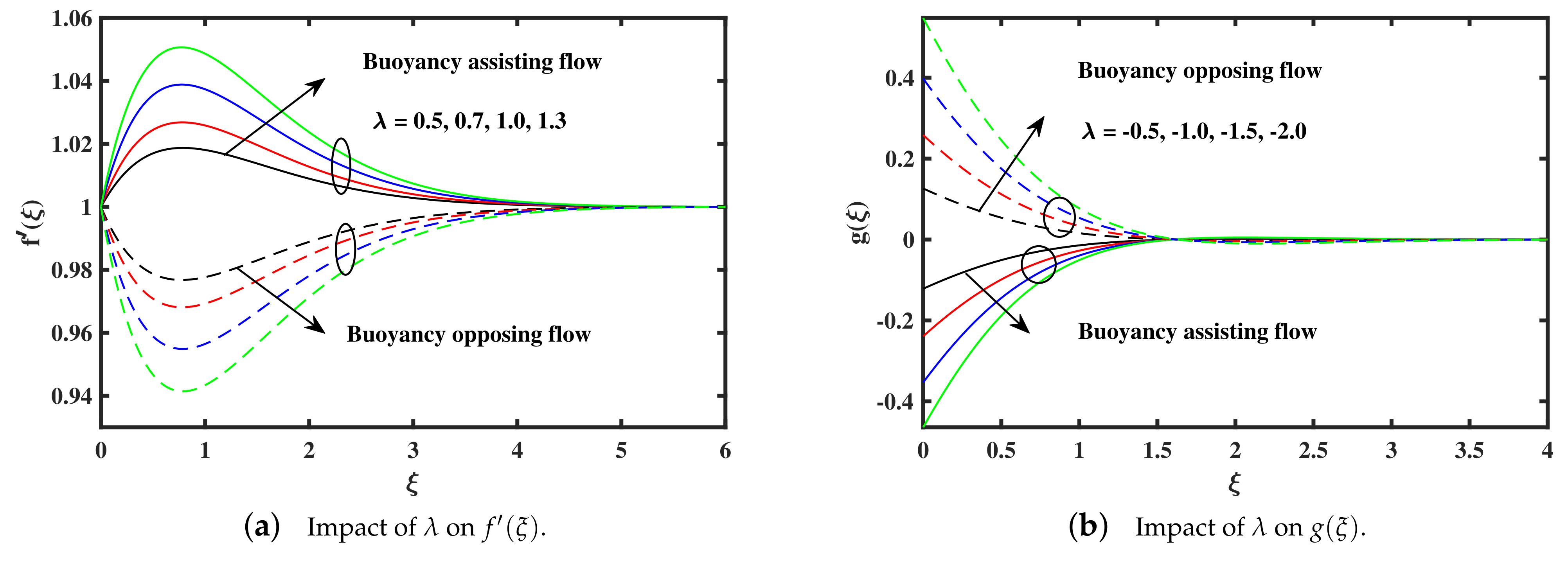
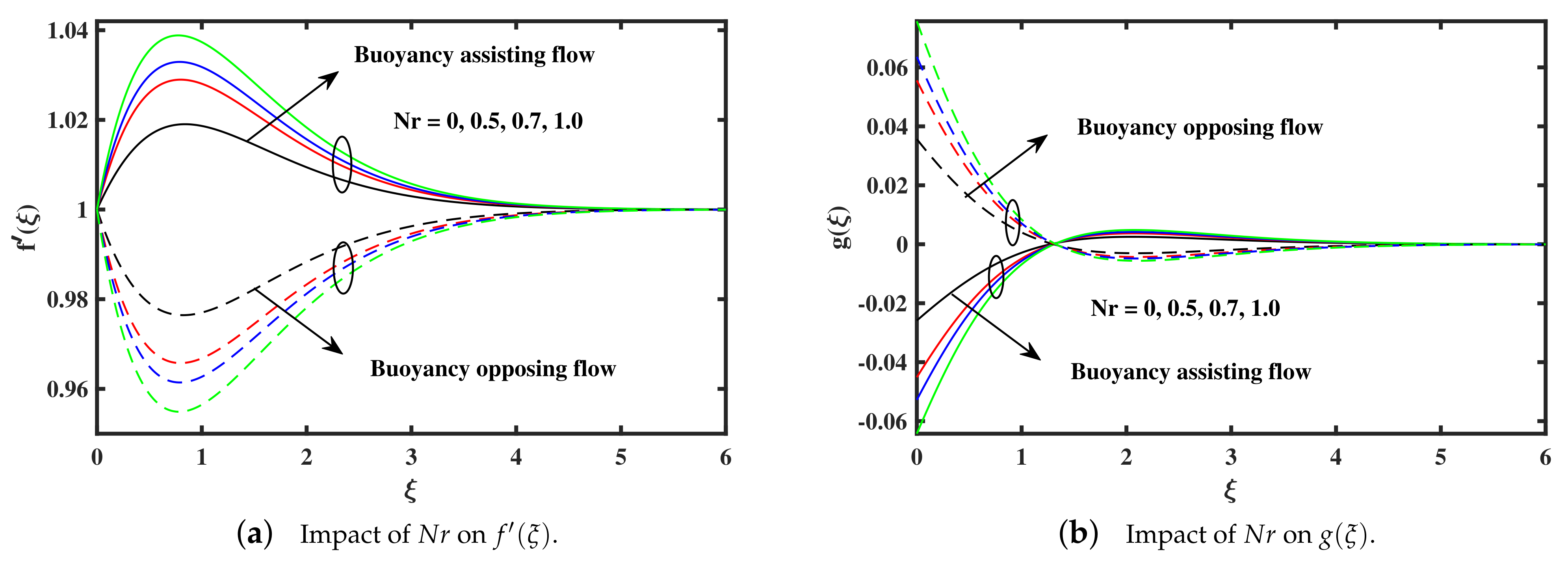
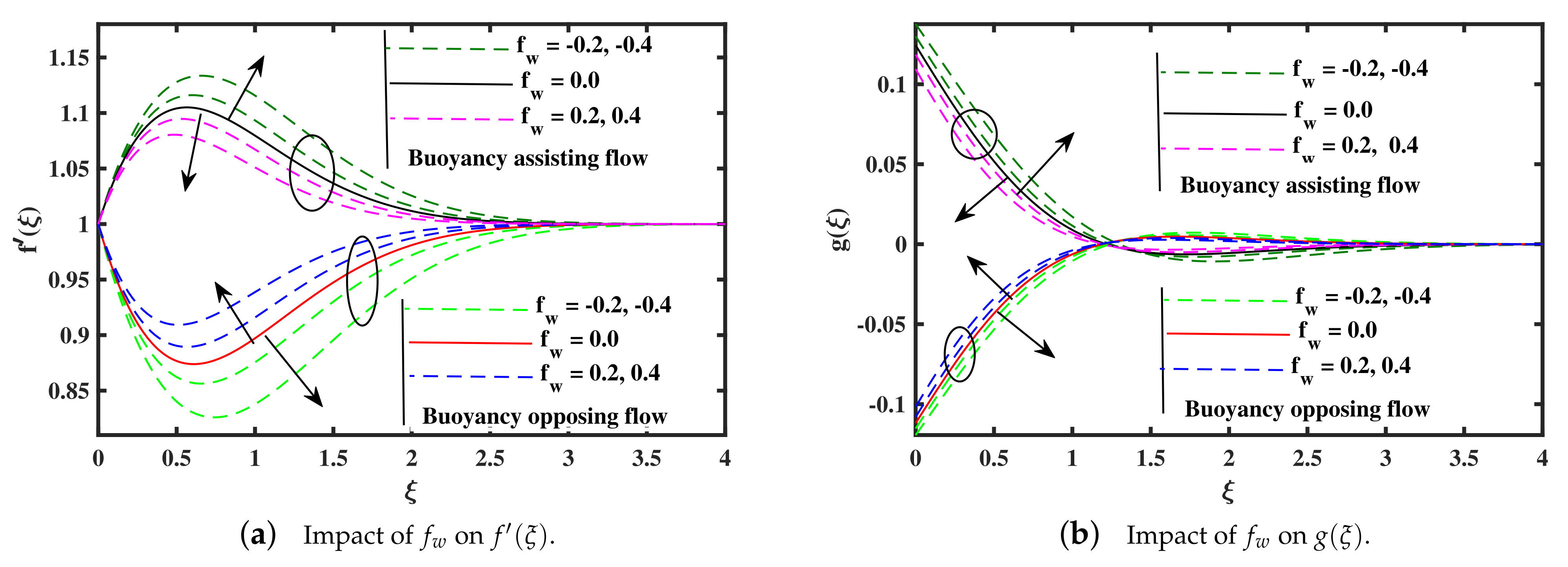
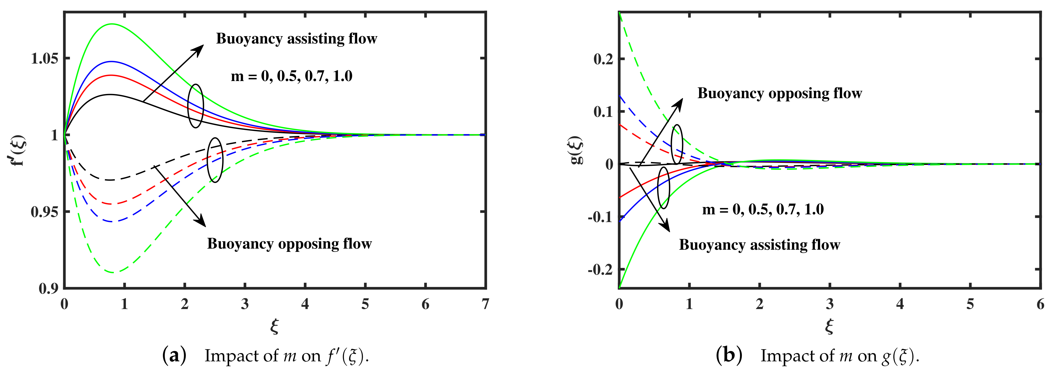
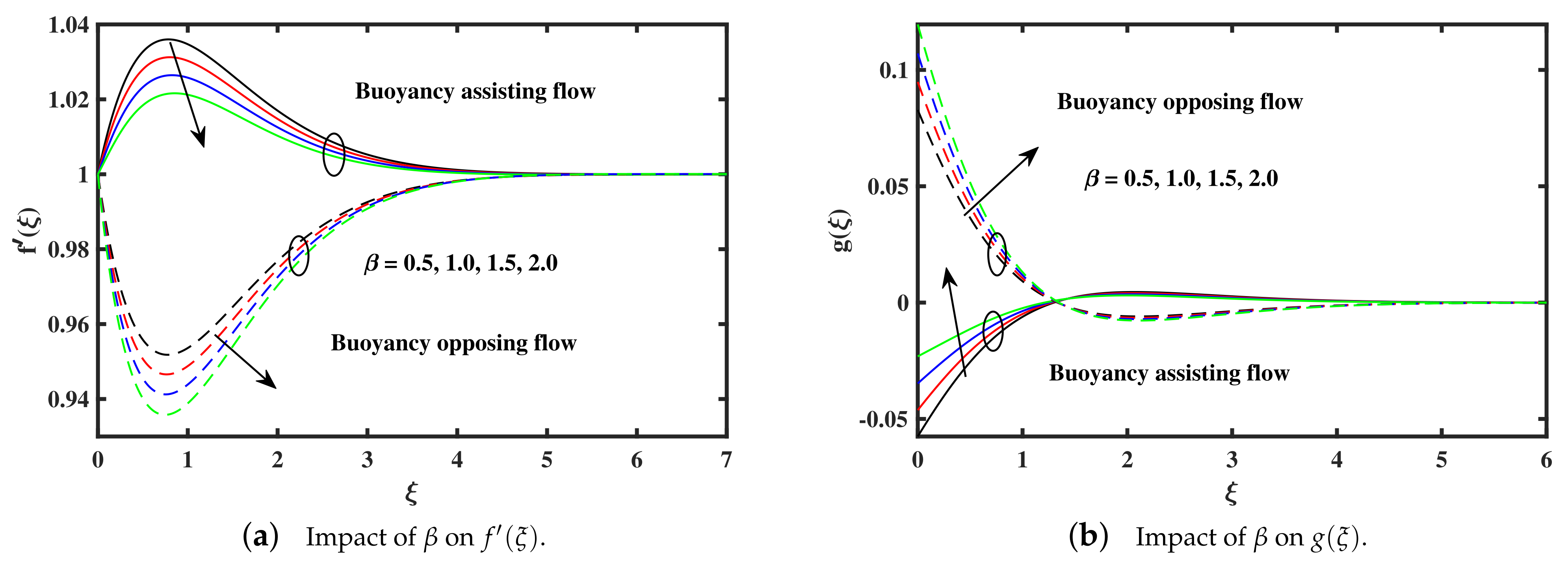
• The micro rotation $g\left(\xi \right)$ and velocity $f^{\prime }\left(\xi \right)$ enhance against the rising of microrotation concentration $\left(m\right)$, injection $\left(f_w\right)$, and buoyancy forces($Rb,\lambda ,Nr)$ parameters in assisting case, but the inverse behaviour is reported in opposing case.
• The microrotation and velocity reduce along growing of micropolar material, and suction ($f_w$) parameters in case of assisting, but opposite phenomena is seen in case of opposing.
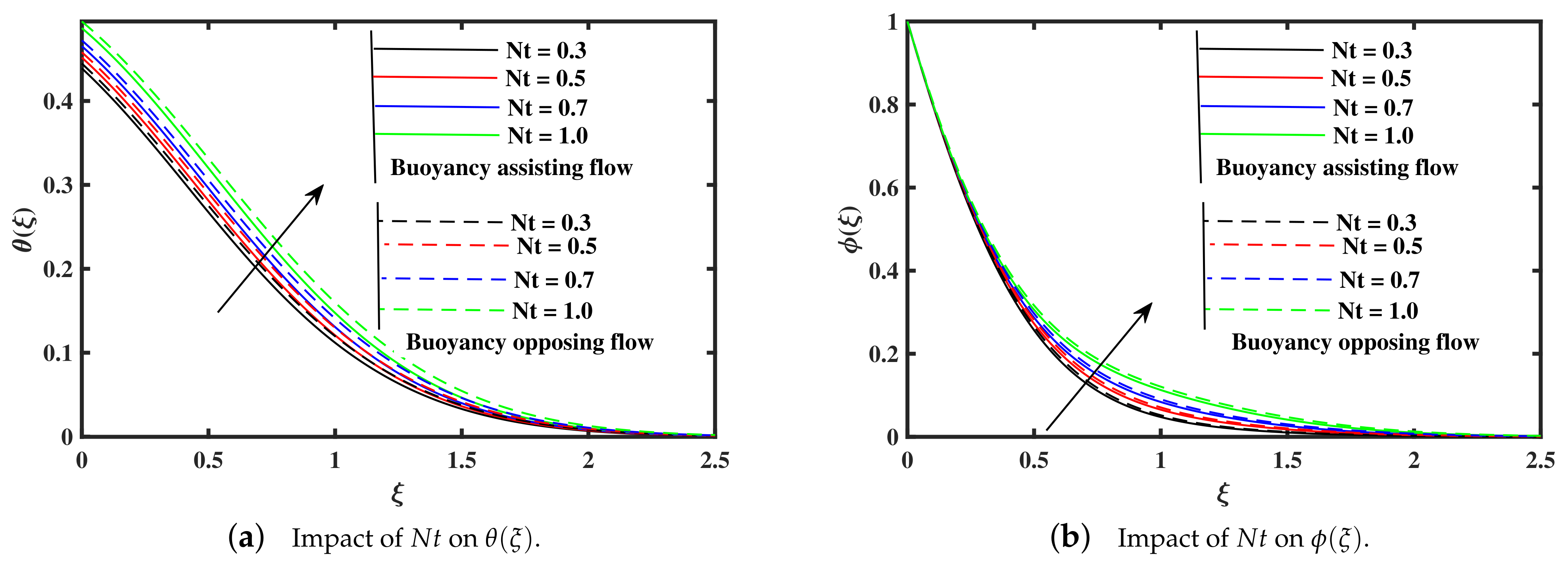
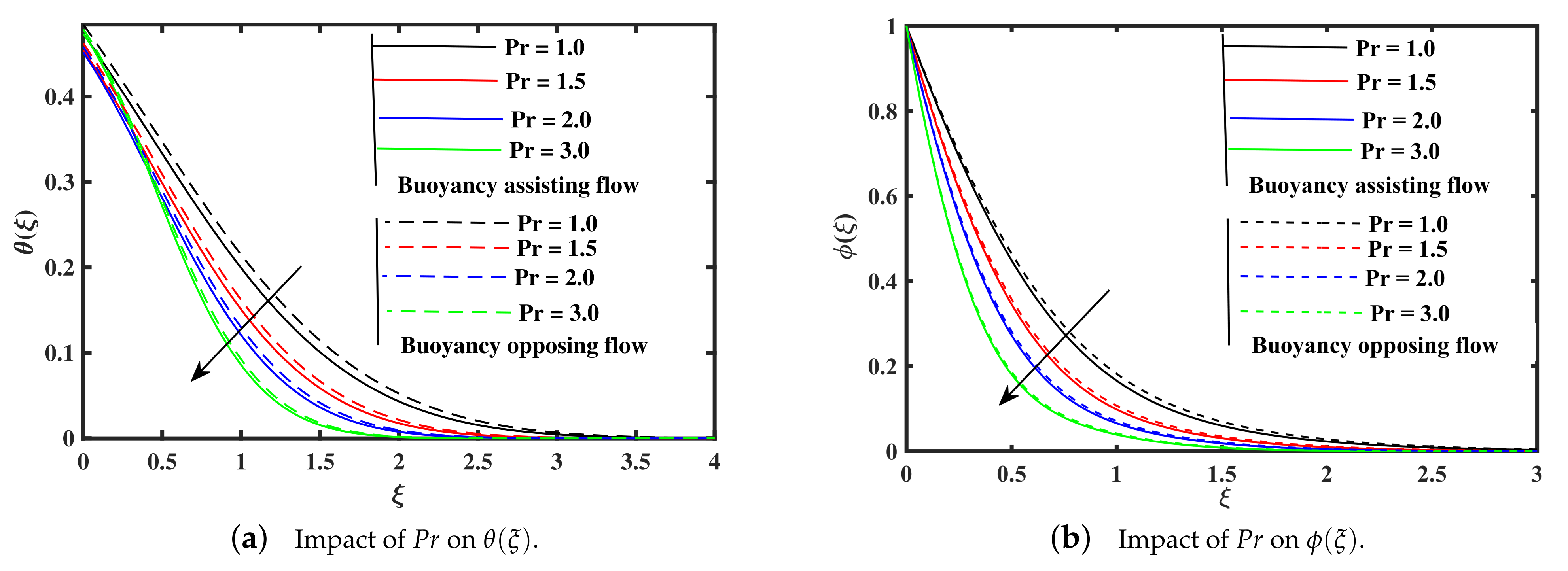
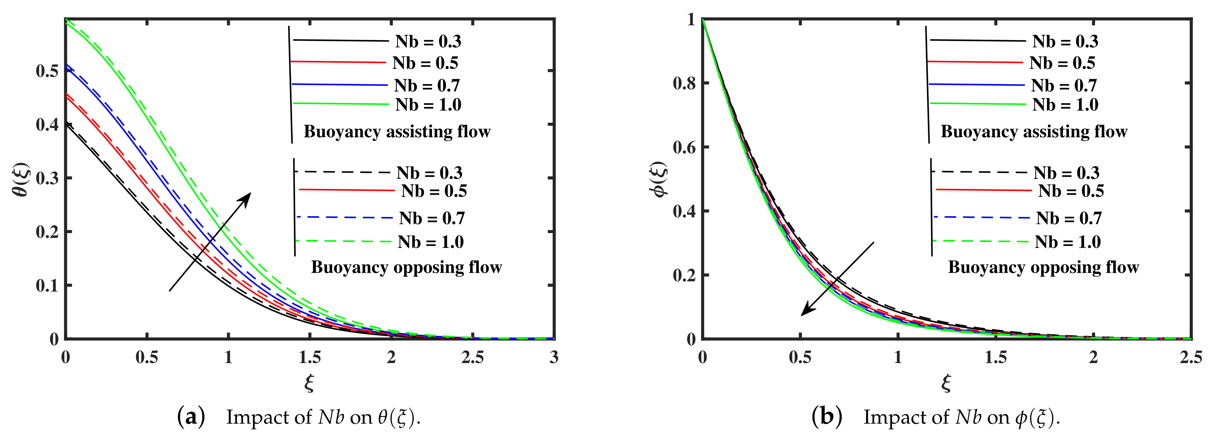
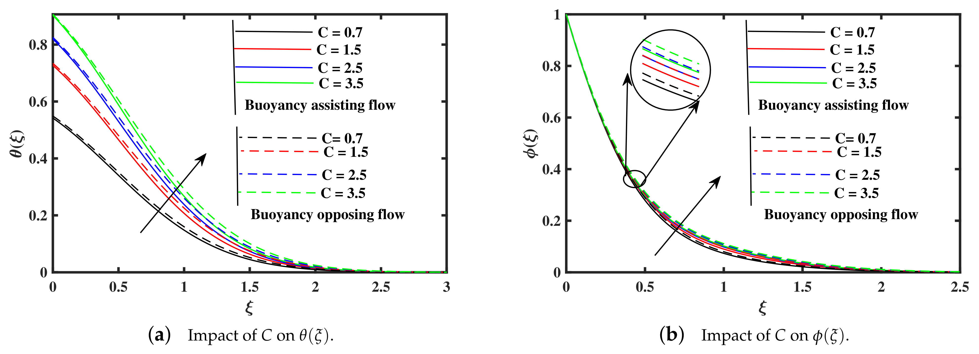
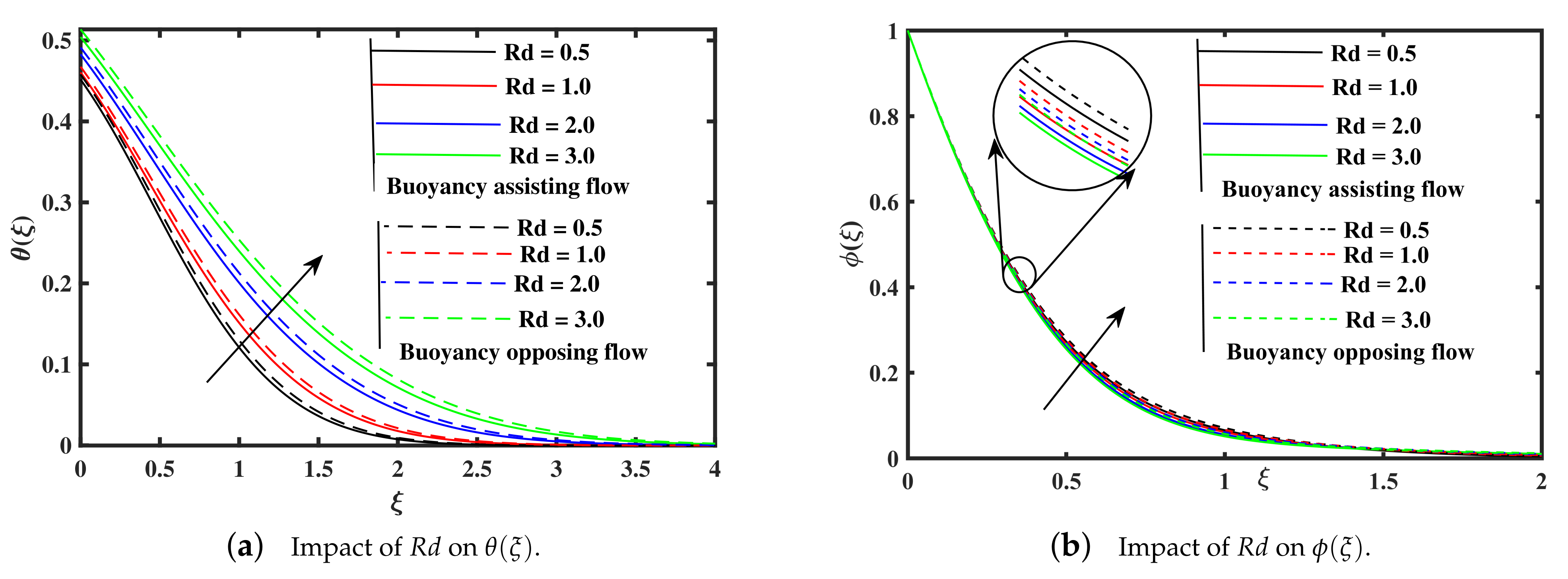
• The distribution of temperature shows a rising along the growing of the Brownian motion, thermophoresis, Biot number, and radiation parameters, while the temperature declined with the elevation of Prandtl number, and rate of heat transfer is lower in assisting case.
• The tiny particles concentration distribution $\varphi \left(\xi \right)$ demonstrates a decrease along the raising of Prandtl number, and Brownian motion, while the non-dimensional concentration enhance with upgrading of radiation, Biot number, and thermophoresis parameters. Moreover, it is noted that the impact of opposing case on the non-dimensional concentration profile is high as compared to assisting case.
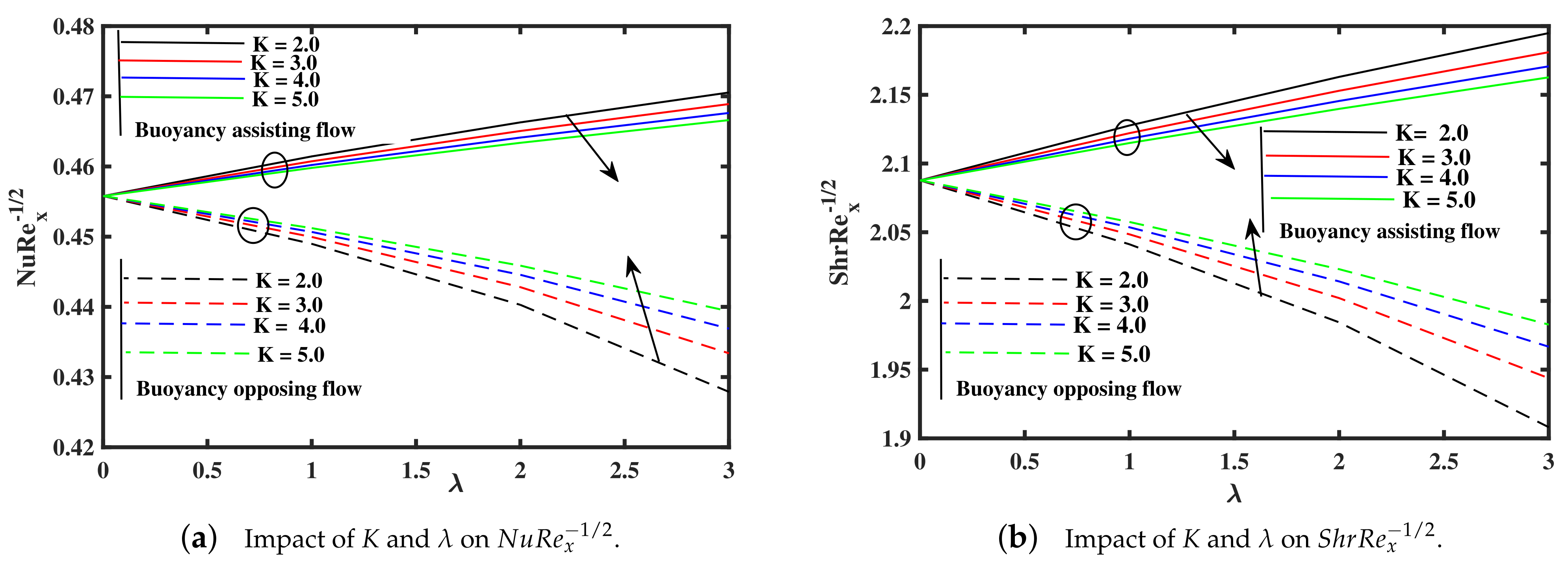
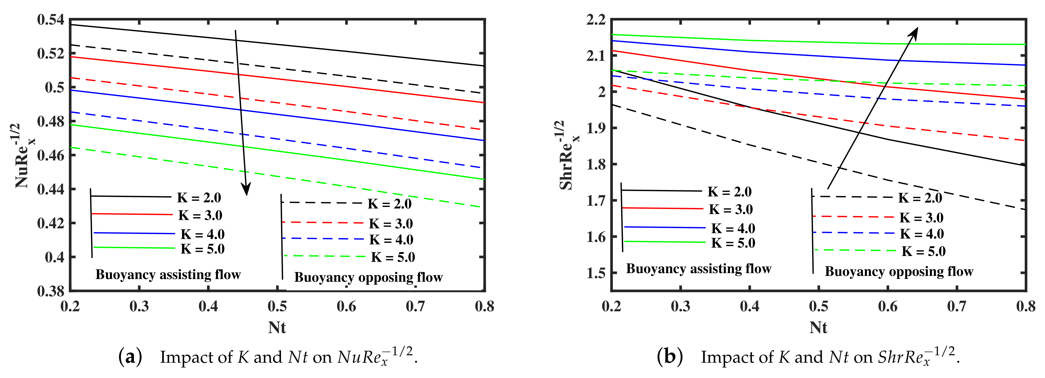
• The Sherwood and Nusselt numbers coefficient rate become smaller against higher K in assisting case, but opposing case exhibit inverse trend, and decreased by mean of rising $\lambda$ in opposing case, but reverse phenomena is reported in assisting case.
• An increase in thermophoresis and material parameters, decline in Nusselt number is noted, and Sherwood number show an opposite affects along elevation of K.
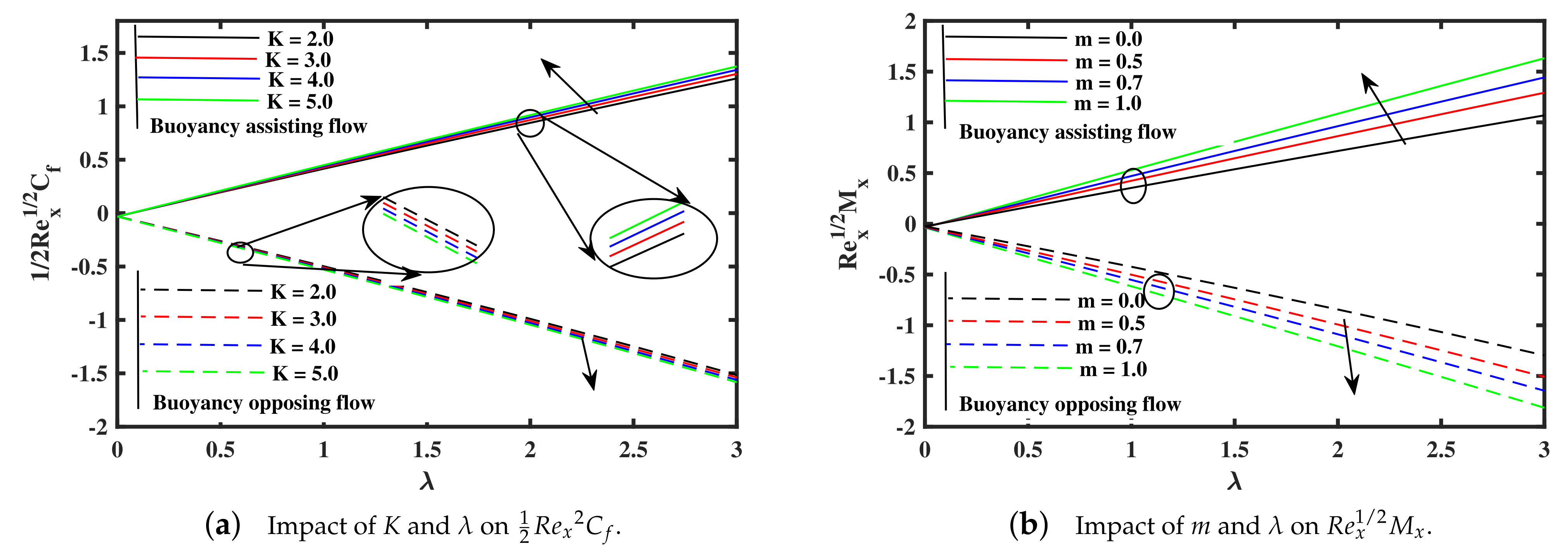
• The skin friction factor rise, by mean of growing $\lambda$ and K in assisting case, but opposing case exhibits an opposite trend. Additionally, the rate of couple stress increased against rising of $\lambda$ and m in assisting case, but opposing case shows inverse behavior.

References

- Hayat, T.; Ahmad, S.; Khan, M.I.; Alsaedi, A. Simulation of ferromagnetic nanomaterial flow of Maxwell fluid. Results Phys. 2018, 8, 34–40. [Google Scholar] [CrossRef]
- Godson, L.; Raja, B.; Lal, D.M.; Wongwises, S.E.A. Enhancement of heat transfer using nanofluids—An overview. Renew. Sustain. Energy Rev. 2010, 14, 629–641. [Google Scholar] [CrossRef]
- Ali, L.; Liu, X.; Ali, B.; Mujeed, S.; Abdal, S.; Khan, S.A. Analysis of Magnetic Properties of Nano-Particles Due to a Magnetic Dipole in Micropolar Fluid Flow over a Stretching Sheet. Coatings 2020, 10, 170. [Google Scholar] [CrossRef] [Green Version]
- Stephen, P.S. Low Viscosity Magnetic Fluid Obtained by the Colloidal Suspension of Magnetic Particles. U.S. Patent 3,215,572, 2 November 1965. [Google Scholar]
- Albrecht, T.; Bührer, C.; Fähnle, M.; Maier, K.; Platzek, D.; Reske, J. First observation of ferromagnetism and ferromagnetic domains in a liquid metal. Appl. Phys. A 1997, 65, 215–220. [Google Scholar] [CrossRef]
- Andersson, H.; Valnes, O. Flow of a heated ferrofluid over a stretching sheet in the presence of a magnetic dipole. Acta Mech. 1998, 128, 39–47. [Google Scholar] [CrossRef]
- Shliomis, M. Comment on “ferrofluids as thermal ratchets”. Phys. Rev. Lett. 2004, 92, 1–6. [Google Scholar] [CrossRef]
- Neuringer, J.L.; Rosensweig, R.E. Ferrohydrodynamics. Phys. Fluids 1964, 7, 1927–1937. [Google Scholar] [CrossRef]
- Bailey, R. Lesser known applications of ferrofluids. J. Magn. Magn. Mater. 1983, 39, 178–182. [Google Scholar] [CrossRef]
- Mehmood, Z.; Mehmood, R.; Iqbal, Z. Numerical investigation of micropolar Casson fluid over a stretching sheet with internal heating. Commun. Theor. Phys. 2017, 67, 443. [Google Scholar] [CrossRef]
- Eringen, A.C. Theory of micropolar fluids. J. Math. Mech. 1966, 16, 1–18. [Google Scholar] [CrossRef]
- Izadi, M.; Sheremet, M.A.; Mehryan, S.; Pop, I.; Öztop, H.F.; Abu-Hamdeh, N. MHD thermogravitational convection and thermal radiation of a micropolar nanoliquid in a porous chamber. Int. Commun. Heat Mass Transf. 2020, 110, 104409. [Google Scholar] [CrossRef]
- Izadi, M.; Mohammadi, S.A.; Mehryan, S.; Yang, T.; Sheremet, M.A. Thermogravitational convection of magnetic micropolar nanofluid with coupling between energy and angular momentum equations. Int. J. Heat Mass Transf. 2019, 145, 118748. [Google Scholar] [CrossRef]
- Hassanien, I.; Gorla, R. Heat transfer to a micropolar fluid from a non-isothermal stretching sheet with suction and blowing. Acta Mech. 1990, 84, 191–199. [Google Scholar] [CrossRef]
- Turkyilmazoglu, M. Flow of a micropolar fluid due to a porous stretching sheet and heat transfer. Int. J. Non-Linear Mech. 2016, 83, 59–64. [Google Scholar] [CrossRef]
- Abdal, S.; Ali, B.; Younas, S.; Ali, L.; Mariam, A. Thermo-Diffusion and Multislip Effects on MHD Mixed Convection Unsteady Flow of Micropolar Nanofluid over a Shrinking/Stretching Sheet with Radiation in the Presence of Heat Source. Symmetry 2020, 12, 49. [Google Scholar] [CrossRef] [Green Version]
- Seth, G.; Bhattacharyya, A.; Kumar, R.; Chamkha, A. Entropy generation in hydromagnetic nanofluid flow over a non-linear stretching sheet with Navier’s velocity slip and convective heat transfer. Phys. Fluids 2018, 30, 122003. [Google Scholar] [CrossRef]
- Seth, G.; Bhattacharyya, A.; Mishra, M. Study of partial slip mechanism on free convection flow of viscoelastic fluid past a nonlinearly stretching surface. Comput. Therm. Sci. 2018, 11, 107–119. [Google Scholar] [CrossRef]
- Crane, L.J. Flow past a stretching plate. Z. Angew. Math. Phys. ZAMP 1970, 21, 645–647. [Google Scholar] [CrossRef]
- Faraz, F.; Imran, S.M.; Ali, B.; Haider, S. Thermo-diffusion and multi-slip effect on an axisymmetric Casson flow over a unsteady radially stretching sheet in the presence of chemical reaction. Processes 2019, 7, 851. [Google Scholar] [CrossRef] [Green Version]
- Gupta, P.; Gupta, A. Heat and mass transfer on a stretching sheet with suction or blowing. Can. J. Chem. Eng. 1977, 55, 744–746. [Google Scholar] [CrossRef]
- Ashraf, M.; Bashir, S. Numerical simulation of MHD stagnation point flow and heat transfer of a micropolar fluid towards a heated shrinking sheet. Int. J. Numer. Methods Fluids 2012, 69, 384–398. [Google Scholar] [CrossRef]
- Gupta, D.; Kumar, L.; Bég, O.A.; Singh, B. Finite element analysis of melting effects on MHD stagnation-point non-Newtonian flow and heat transfer from a stretching/shrinking sheet. AIP Conf. Proc. 2019, 2061, 020024. [Google Scholar] [CrossRef]
- Ghasemi, S.; Hatami, M. Solar radiation effects on MHD stagnation point flow and heat transfer of a nanofluid over a stretching sheet. Case Stud. Therm. Eng. 2021, 25, 100898. [Google Scholar] [CrossRef]
- Zainal, N.A.; Nazar, R.; Naganthran, K.; Pop, I. Unsteady EMHD stagnation point flow over a stretching/shrinking sheet in a hybrid Al2O3-Cu/H2O nanofluid. Int. Commun. Heat Mass Transf. 2021, 123, 105205. [Google Scholar] [CrossRef]
- Chiam, T.C. Stagnation-point flow towards a stretching plate. J. Phys. Soc. Jpn. 1994, 63, 2443–2444. [Google Scholar] [CrossRef]
- Amjad, M.; Zehra, I.; Nadeem, S.; Abbas, N. Thermal analysis of Casson micropolar nanofluid flow over a permeable curved stretching surface under the stagnation region. J. Therm. Anal. Calorim. 2021, 143, 2485–2497. [Google Scholar] [CrossRef]
- Izadi, M.; Pour, S.H.; Yasuri, A.K.; Chamkha, A.J. Mixed convection of a nanofluid in a three-dimensional channel. J. Therm. Anal. Calorim. 2019, 136, 2461–2475. [Google Scholar] [CrossRef]
- Izadi, M.; Oztop, H.F.; Sheremet, M.A.; Mehryan, S.; Abu-Hamdeh, N. Coupled FHD–MHD free convection of a hybrid nanoliquid in an inversed T-shaped enclosure occupied by partitioned porous media. Numer. Heat Transf. Part A Appl. 2019, 76, 479–498. [Google Scholar] [CrossRef]
- Ali, B.; Naqvi, R.A.; Ali, L.; Abdal, S.; Hussain, S. A comparative description on time-dependent rotating magnetic transport of a water base liquid H2O with hybrid nano-materials Al2O3-Cu and Al2O3-TiO2 over an extending sheet using Buongiorno model: Finite element approach. Chin. J. Phys. 2021, 70, 125–139. [Google Scholar] [CrossRef]
- Ali, B.; Nie, Y.; Hussain, S.; Habib, D.; Abdal, S. Insight into the dynamics of fluid conveying tiny particles over a rotating surface subject to Cattaneo–Christov heat transfer, Coriolis force, and Arrhenius activation energy. Comput. Math. Appl. 2021, 93, 130–143. [Google Scholar] [CrossRef]
- Choi, S.U.; Eastman, J.A. Enhancing Thermal Conductivity of Fluids with Nanoparticles; Technical Report; Argonne National Lab.: Lemont, IL, USA, 1995. [Google Scholar]
- Izadi, M.; Javanahram, M.; Zadeh, S.M.H.; Jing, D. Hydrodynamic and heat transfer properties of magnetic fluid in porous medium considering nanoparticle shapes and magnetic field-dependent viscosity. Chin. J. Chem. Eng. 2020, 28, 329–339. [Google Scholar] [CrossRef]
- Izadi, M.; Shahmardan, M.; Rashidi, A. Study on thermal and hydrodynamic indexes of a nanofluid flow in a micro heat sink. Transp. Phenom Nano Micro Scales 2013, 1, 53–63. [Google Scholar]
- Bachok, N.; Ishak, A.; Pop, I. Unsteady boundary-layer flow and heat transfer of a nanofluid over a permeable stretching/shrinking sheet. Int. J. Heat Mass Transf. 2012, 55, 2102–2109. [Google Scholar] [CrossRef]
- Wen, D.; Lin, G.; Vafaei, S.; Zhang, K. Review of nanofluids for heat transfer applications. Particuology 2009, 7, 141–150. [Google Scholar] [CrossRef]
- Ur Rasheed, H.; Saleem, S.; Islam, S.; Khan, Z.; Khan, W.; Firdous, H.; Tariq, A. Effects of Joule Heating and Viscous Dissipation on Magnetohydrodynamic Boundary Layer Flow of Jeffrey Nanofluid over a Vertically Stretching Cylinder. Coatings 2021, 11, 353. [Google Scholar] [CrossRef]
- Ali, B.; Pattnaik, P.; Naqvi, R.A.; Waqas, H.; Hussain, S. Brownian motion and thermophoresis effects on bioconvection of rotating Maxwell nanofluid over a Riga plate with Arrhenius activation energy and Cattaneo-Christov heat flux theory. Therm. Sci. Eng. Prog. 2021, 23, 100863. [Google Scholar] [CrossRef]
- Sadiq, K.; Jarad, F.; Siddique, I.; Ali, B. Soret and Radiation Effects on Mixture of Ethylene Glycol-Water (50%-50%) Based Maxwell Nanofluid Flow in an Upright Channel. Complexity 2021, 2021, 5927070. [Google Scholar] [CrossRef]
- Ali, B.; Hussain, S.; Shafique, M.; Habib, D.; Rasool, G. Analyzing the interaction of hybrid base liquid C2H6O2-H2O with hybrid nano-material Ag-MoS2 for unsteady rotational flow referred to an elongated surface using modified Buongiorno’s model: FEM simulation. Math. Comput. Simul. 2021, 190, 57–74. [Google Scholar] [CrossRef]
- Ray, A.K.; Vasu, B.; Bég, O.A.; Gorla, R.S.; Murthy, P. Homotopy semi-numerical modeling of non-Newtonian nanofluid transport external to multiple geometries using a revised Buongiorno Model. Inventions 2019, 4, 54. [Google Scholar] [CrossRef] [Green Version]
- Ali, L.; Liu, X.; Ali, B.; Mujeed, S.; Abdal, S.; Mutahir, A. The Impact of Nanoparticles Due to Applied Magnetic Dipole in Micropolar Fluid Flow Using the Finite Element Method. Symmetry 2020, 12, 520. [Google Scholar] [CrossRef] [Green Version]
- Majeed, A.; Zeeshan, A.; Hayat, T. Analysis of magnetic properties of nanoparticles due to applied magnetic dipole in aqueous medium with momentum slip condition. Neural Comput. Appl. 2019, 31, 189–197. [Google Scholar] [CrossRef]
- Khan, S.A.; Nie, Y.; Ali, B. Stratification and Buoyancy Effect of Heat Transportation in Magnetohydrodynamics Micropolar Fluid Flow Passing over a Porous Shrinking Sheet Using the Finite Element Method. J. Nanofluids 2019, 8, 1640–1647. [Google Scholar] [CrossRef]
- Khan, S.A.; Nie, Y.; Ali, B. Multiple slip effects on MHD unsteady viscoelastic nano-fluid flow over a permeable stretching sheet with radiation using the finite element method. SN Appl. Sci. 2020, 2, 1–14. [Google Scholar] [CrossRef] [Green Version]
- Hayat, T.; Ahmad, S.; Khan, M.I.; Alsaedi, A. Exploring magnetic dipole contribution on radiative flow of ferromagnetic Williamson fluid. Results Phys. 2018, 8, 545–551. [Google Scholar] [CrossRef]
- Ali, B.; Siddique, I.; Khan, I.; Masood, B.; Hussain, S. Magnetic dipole and thermal radiation effects on hybrid base micropolar CNTs flow over a stretching sheet: Finite element method approach. Results Phys. 2021, 25, 104145. [Google Scholar] [CrossRef]
- Majeed, A.; Zeeshan, A.; Ellahi, R. Unsteady ferromagnetic liquid flow and heat transfer analysis over a stretching sheet with the effect of dipole and prescribed heat flux. J. Mol. Liq. 2016, 223, 528–533. [Google Scholar] [CrossRef]
- Abdal, S.; Hussain, S.; Ahmad, F.; Ali, B. Hydromagnetic Stagnation Point Flow OF Micropolar Fluids Due To A Porous Stretching Surface With Radiation And Viscous Dissipation. Sci. Int. 2015, 27, 3965–3971. [Google Scholar]
- Ali, B.; Yu, X.; Sadiq, M.T.; Rehman, A.U.; Ali, L. A Finite Element Simulation of the Active and Passive Controls of the MHD Effect on an Axisymmetric Nanofluid Flow with Thermo-Diffusion over a Radially Stretched Sheet. Processes 2020, 8, 207. [Google Scholar] [CrossRef] [Green Version]
- Jyothi, K.; Reddy, P.S.; Reddy, M.S. Carreau nanofluid heat and mass transfer flow through wedge with slip conditions and nonlinear thermal radiation. J. Braz. Soc. Mech. Sci. Eng. 2019, 41, 1–15. [Google Scholar] [CrossRef]
- Reddy, J.N. Solutions Manual for an Introduction to the Finite Element Method; McGraw-Hill: New York, NY, USA, 1993; p. 41. [Google Scholar]
- Ali, B.; Naqvi, R.A.; Nie, Y.; Khan, S.A.; Sadiq, M.T.; Rehman, A.U.; Abdal, S. Variable Viscosity Effects on Unsteady MHD an Axisymmetric Nanofluid Flow over a Stretching Surface with Thermo-Diffusion: FEM Approach. Symmetry 2020, 12, 234. [Google Scholar] [CrossRef] [Green Version]
- Ali, L.; Liu, X.; Ali, B.; Mujeed, S.; Abdal, S. Finite Element Simulation of Multi-Slip Effects on Unsteady MHD Bioconvective Micropolar nanofluid Flow over a Sheet with Solutal and Thermal Convective Boundary Conditions. Coatings 2019, 9, 842. [Google Scholar] [CrossRef]
- Ali, B.; Nie, Y.; Khan, S.A.; Sadiq, M.T.; Tariq, M. Finite element simulation of multiple slip effects on MHD unsteady maxwell nanofluid flow over a permeable stretching sheet with radiation and thermo-diffusion in the presence of chemical reaction. Processes 2019, 7, 628. [Google Scholar] [CrossRef] [Green Version]
- Ishak, A.; Nazar, R.; Pop, I. Mixed convection boundary layers in the stagnation-point flow toward a stretching vertical sheet. Meccanica 2006, 41, 509–518. [Google Scholar] [CrossRef] [Green Version]
- Mahapatra, T.R.; Gupta, A. Heat transfer in stagnation-point flow towards a stretching sheet. Heat Mass Transf. 2002, 38, 517–521. [Google Scholar] [CrossRef]
- Khan, Z.H.; Khan, W.A.; Qasim, M.; Shah, I.A. MHD stagnation point ferrofluid flow and heat transfer toward a stretching sheet. IEEE Trans. Nanotechnol. 2013, 13, 35–40. [Google Scholar] [CrossRef]
- Nazar, R.; Amin, N.; Filip, D.; Pop, I. Unsteady boundary layer flow in the region of the stagnation point on a stretching sheet. Int. J. Eng. Sci. 2004, 42, 1241–1253. [Google Scholar] [CrossRef] [Green Version]
- Qasim, M.; Khan, I.; Shafie, S. Heat transfer in a micropolar fluid over a stretching sheet with Newtonian heating. PLoS ONE 2013, 8, e59393. [Google Scholar] [CrossRef] [Green Version]
- Tripathy, R.; Dash, G.; Mishra, S.; Hoque, M.M. Numerical analysis of hydromagnetic micropolar fluid along a stretching sheet embedded in porous medium with non-uniform heat source and chemical reaction. Eng. Sci. Technol. Int. J. 2016, 19, 1573–1581. [Google Scholar] [CrossRef] [Green Version]