Abstract
Due to its excellent toughness and stiffness in cryogenic conditions, 9% nickel steel is applied to LNG storage facilities, and its usage is increasing as a result of changes in environmental regulations. A study was conducted on the development of a predictive model to optimize the laser welding process of 9% nickel steel, and two prediction models were developed using one hundred data points obtained through experiments. A global regression model used as a general prediction model and a modified regression model using the p-value of the analysis of variance were developed, and their prediction performance was compared. It was found that the modified regression model was superior to the global regression model in terms of predicting the bead shape, including parameters such as penetration depth, bead height, and area ratio.
1. Introduction
Ship emission regulations are being strengthened in accordance with global environmental regulations to prevent climate change. The shipbuilding industry continues to study the use of liquefied natural gas (LNG) for marine fuels as an alternative to conventional fossil fuels [1,2]. With the application of LNG fuel, the material used for fuel tanks has also been changing, with the stainless steel 304L, aluminum alloy 5083-0, and Invar that were used in low temperature environments in the past being replaced with 9% nickel steel to reduce costs [3]. The 9% nickel steel is used as a material for cryogenic tanks such as LNG, and recently has been used as a material for LNG fuel tanks because of its relatively high yield strength/tensile strength compared to other materials. There are several factors that determine the thickness of an LNG fuel tank, among which the minimum yield/tensile strength is an important factor. The 9% nickel steel has the disadvantage that after welding, the welding strength is reduced and the tank thickness increases [4]. By applying laser welding, the strength of this part can be increased and the thickness of the tank reduced [5]. Laser welding is a welding method in which a material is melted with a high density of energy focused on a very small point [6]. In the process of laser welding, laser focused light reaches the surface of the material to be welded and is mostly lost through surface reflection, but a small amount of absorbed energy rapidly heats the material to generate high-temperature metal vapor and ions (laser plasma). In the welding process, when the laser focused light has a predetermined energy density, a keyhole, which is a small hole, is created in the material. When the keyhole is deepened, the laser light causes continuous reflection, increasing the energy transfer effect used for welding. As the laser beam is in continuous mode and welding proceeds, the molten metal around the keyhole adheres to some walls by surface tension, and some of it accumulates under the keyhole under the influence of gravity and solidifies to form a welding bead [7]. Laser welding using the keyhole phenomenon has a different welding mechanism than the conventional arc welding method. In arc welding, the melting of the material and the formation of the weld are performed by heat conduction, so the melting isotherm moves outside the heat source [8]. In addition, since a large amount of energy must be administered to obtain a predetermined penetration depth, excess energy that is not directly used for melting of the material increases the size of the heat-affected zone. As a result, in arc welding, the penetration depth is low, the welding must be repeated several times, and the welding speed is also very slow. However, keyhole welding is a high-speed welding method of direct input in the thickness direction of the material rather than gradual heat transfer from the surface to the material when welding energy is transferred to the material [9,10].
The advantages of laser welding are as follows. In laser welding, narrow and deep welds can be obtained and, if the power is sufficient, considerably deep welds can be easily obtained with only one weld. It is very advantageous in productivity because the process of welding grooves and the use of welding rods can be excluded. In addition, the laser welding method can be carried out with little energy. Using less energy in welding means that the deformation of the material after welding can be minimized. If the amount of deformation is small, the pre- and post-welding treatment process, that is, the scale and load of the welding jig can be reduced, and since the work for shaping the welding product can be omitted or reduced, the production cost can be significantly reduced. In addition, metallurgically, it is possible to reduce the embrittlement of the heat-affected zone and reduce the coarsening of microstructures occurring near the weld zone. For this reason, laser welding technology is widely used for dissimilar metal welding [11,12]. Despite the advantages listed above, laser welding has limitations that cannot be overlooked. In laser welding, since the diameter of the focal point is about 0.5 mm, precise alignment of the weld is required. An additional jig is introduced for the alignment of these welds, which is also a factor that increases the cost of production equipment. Excessive gap opening causes welding defects such as depression of the bead after welding, therefore cracking the welding bead during the forming process or shortening the product fatigue life [13]. In addition, since the temperature gradient of the weld is very large compared to other welding techniques, there is a high probability of high temperature cracking in the center of the weld zone [14,15]. Management of welding conditions, etc., is very important in order to suppress the high-temperature cracking of such a weld zone.
At the manufacturing site, laser welding is performed by an automated system. The most important thing in the automation of the welding process is to determine the conditions that can enable stable welding over a wide welding range. A prediction model is needed to derive welding conditions suitable for the characteristics of a product, and many studies that sought to develop such prediction models have been conducted. More recently, machine learning-based prediction algorithms have been developed from the inferences of the empirical equations derived through many previous experiments, based on the carbon content for the preheating and post-heat treatment of welding materials [16,17]. However, even when the same process of welding technology is used, the welding results will differ depending on the type of material and heat source characteristics, making it difficult to use a general prediction model. Recently, as the industrial application of 9% nickel steel has increased, related research is increasing.
The welding strength and fatigue life of 9% nickel steel are widely predicted using computer simulation techniques, and the effectiveness of using FEM (finite element analysis) to predict the deformation of a welding part of 9% nickel steel applied to offshore LNG storage has been reported [18]. Park [19] conducted a study on predicting high-temperature cracking in laser welds of 9% nickel steel using regression analysis and response surface analysis. In addition, there was a study conducted to predict the hardness and tensile stress of a weld zone using a mathematical model and FEM according to the number of elements contained in the steel [20]. Most studies focus on predicting the mechanical properties of 9% nickel steel through mathematical or FEM analysis. Yet in practice, problems such as welding deformation and welding defects arise from the bead geometry. Poor welding, under-fill, and lack of fusion can be predicted through the weld shape, and to address this, a bead shape prediction is necessary. Recently, prediction technologies using algorithms such as machine learning, deep learning, and neural networks have also been developed. This prediction technology is based on a mathematical model, and research on improving the predictive performance of the mathematical model needs to be ongoing. Bead shape prediction technology can provide empirical knowledge to minimize welding defects. Selection of a prediction model is important in predicting the bead shape of a specific material; the right model can secure excellent prediction performance. In this study, three models have been developed. The first is a global regression model and a modified regression model (local regression model), the second is a model developed through the correlation of the bead shape, and the third is a model developed through cluster analysis. Prediction performance comparison was performed by applying the regression, clustering, and correlation models used as general prediction models for 9% nickel steel bead geometry prediction. In Part 1, the global regression model was developed and the performance improvement was compared with the modified regression model in which statistical techniques were introduced.
2. Welding Experiment for Model Development
The purpose of this study is to compare and evaluate the performance of various models in predicting the bead shape of 9% nickel steel. Various predictive models were developed through global regression analysis, modification of global regression, cluster analysis, and correlation analysis. Typically, experiments accumulate data and use them to develop a predictive model from the relationship between input and output variables. A laser welding experiment was performed to secure data for developing a predictive model for bead shape, and four models were developed using the acquired data. In this study, four representative models have been developed and various methods applied to improve the performance of the predictive equation. Figure 1 below depicts the overall procedure for creating and evaluating a mathematical model.
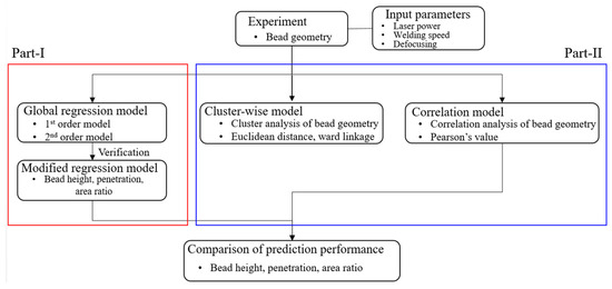
Figure 1.
Research flow for developing predictive model.
Three input variables were assumed: laser power (), welding speed (), and defocusing (focus position ()). Laser power () and welding speed () are important parameters for determining the heat input, and defocusing () is a critical variable for the energy density. Based on the results of the three experiments, three variables were used to develop a mathematical model. The linear global regression model and curvilinear global regression model were developed and performance was evaluated through a variance analysis.
2.1. Materials
Approved by international regulations on construction and equipment and equipment of ships carrying liquefied gas in bulk, 9% Ni steel is used as a material for low temperature/cryogenic energy storage/transport ships. Table 1 shows the mechanical properties and chemical composition of 9% Ni steel listed in ASTM (standard specification for pressure vessel plates, alloy steel, quenched and tempered 7, 8, and 9% nickel) A553. As shown in Figure 2, the test specimen for 9% Ni steel bead on plate welding used in the experiment was 15 mm thick and 150 mm × 300 mm.

Table 1.
Mechanical properties and chemical composition of 9% Ni steel.
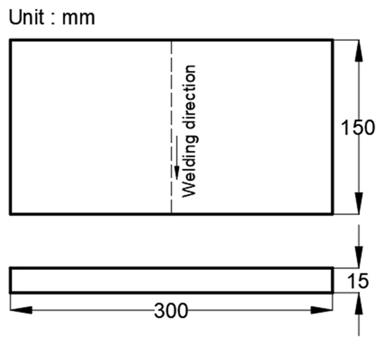
Figure 2.
BOP test specimen dimensions of 9% Ni steel.
2.2. Welding Experiment
Laser welding experiments were conducted to compare and analyze the weld quality of 9% nickel steel. For the experiment, a 5 kW fiber laser welder (Miyachi, Chiba, Japan, model ML-6950A) was used and the whole system was constructed using a robot system (Yaskawa, Kitakyushu, Japan, model: motorman DX100). Figure 3 shows the resonator of the laser welding system, incidental material, optical system, and jig used in the experiment. In welding technology, it is very important to clarify the type of process used, as like the type of base material, this can significantly influence weld quality. In this study, a fiber laser optical system with a specific wavelength of 1070 nm and a focal length of 148.8 mm was used for laser welding of 9% nickel steel. The specifications of the laser welding system are shown in Table 2.
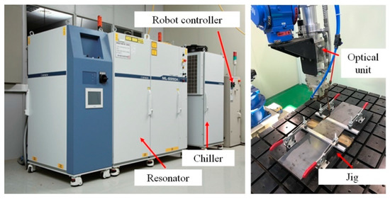
Figure 3.
Configuration of 5 kW fiber laser welding system.
Table 2.
Specifications of 5 kW fiber laser welding machine.
When developing a predictive model, training data are needed in a general supervised learning method. Although a large amount of training data is required to increase the predictive performance of the model, there are limitations to the potential for increasing the amount of data due to limited resources. In this study, an experiment was conducted to secure 100 points of learning data.
In terms of the welding conditions applied in the experiment, as shown in Table 3, bead on plate (BOP) tests with different conditions were performed by adjusting the laser power (), welding speed (), and focus position (). The purpose of this study was to observe the difference in bead geometry according to welding conditions. The maximum laser power generally determines the critical thickness of the weld material. Since the maximum laser power of the fiber laser welding system applied in this study was 5 kW, the maximum limit thickness was predictable to about 15 mm. The basis of the estimation was the information provided in the manual of the Korean Welding Society. The welding parameters and range used in the experiment were appropriately welded through preliminary experiments, and were selected within the range in which the bead shape could be observed.
Table 3.
Experimental conditions of laser welding.
2.3. Measurement of Bead Geometry
Bead geometry measurement was performed to analyze the effect of the welding conditions on the formation of the molten part. Macro cross-sectional inspection is a method employed to smoothly polish the surface of a welded part and perform a chemical solution treatment to examine the structure, pore, penetration, heat affect zone (HAZ), etc. In this study, there were three types of geometry information that could be obtained through a bead cross-section analysis. The first geometry information was the penetration depth, the second was the bead height, and the third was the area ratio. The penetration depth is generally related to the thickness of the weld material, and is also related to keyhole formation. As such, ideal welding can be achieved only if the penetration depth is greater than the thickness of the base material. In addition, securing the bead’s height serves to prevent welding defects such as underfills.
If underfill occurs, the thickness of the welded area becomes thinner than the thickness of the base material. The occurrence of underfill leads to the fracture of the weld zone due to the concentration of stress. When evaluating the quality of welds with the naked eye, the presence of underfill is a very important factor. Figure 4 shows weld failures caused by underfill [21,22].
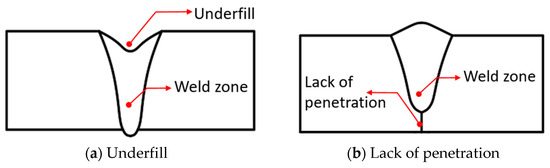
Figure 4.
Laser welding defects observable with bead geometry.
The area ratio of the weld zone is a predictor variable related to weld deformation. The difference in the melting shape of the upper and lower welds of the central axis of the base metal causes weld deformation. As shown in Figure 5, when the molten metal solidifies, contraction force occurs, and deformation occurs due to the difference in the contraction force. This difference in output is related to the area of the melt, and the ratio of the upper and lower melt areas is called the area ratio. Matsuoka [23] found that the bead geometry of the weld zone directly affects the welding deformation and is reported to be based on the expansion and contraction of the weld zone. In addition, it has been reported that the larger the difference in the area of the central axis of the weld zone in the keyhole welding, the larger the angular deformity. For this reason, in this study, a model to predict welding defects such as underfill and welding deformation related to three major points of bead geometry (bead height, penetration depth, and area ratio) was developed.
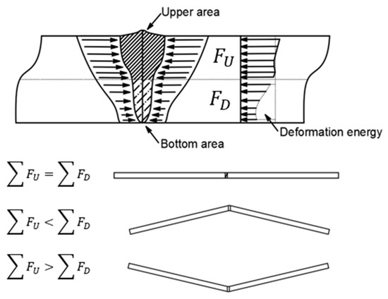
Figure 5.
Mechanism of occurrence of deformation of welds by area ratio (melting zone asymmetry).
2.4. Measurement of Bead Geomtry
To measure bead geometry, the middle parts of the horizontal axis of the experiment specimen are cut to a size of 10 mm × 25 mm size using a wire cutting machine and polished. To make the experiment specimen′s bead geometry clearly visible, Nital (10% HNO3 and ethanol) solution was applied for etching the cross-section of specimens. In addition, an optic microscope system was used for the accurate measurement of bead geometry and actually measured cross-sectional bead geometries. Figure 6 shows the classification and measurement method of bead geometry. A microscope system was also used to support the accurate measurement of the bead geometry, and was actually capable of measuring cross-sectional bead geometries. To accurately measure the bead geometries, bead height, penetration depth and area ratio (upper area per bottom area) were measured by measuring the length of a pixel measuring 0.125 × 0.125 mm. Table 4 shows the data obtained through the experiment. After the welding was performed, the surface bead was observed through a visual test (VT), the shape of the cross-section was observed, and the data without internal pores and cracks were finally selected and used to develop a model. Figure 7 shows the three weld bead shapes obtained through this experiment, and Figure 8 shows the surface bead shape by observing the surface of the specimen for VT.
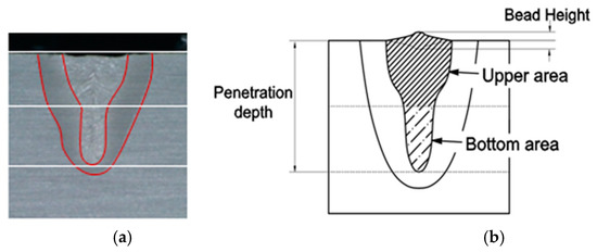
Figure 6.
Classification and measurement method of bead geometry. (a) Laser welding cross-section taken through an optical microscope after the experiment. (b) Measurement point of bead geometry.
Table 4.
Welding condition and experiment results.
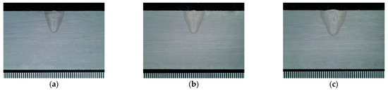
Figure 7.
Bead geometry of 9% Ni steel welded by laser process (a) P: 3 kW, S: 1 m/min, d: 0 mm, (b) P: 4 kW, S: 1 m/min, d: 0 mm, (c) P: 5 kW, S: 1 m/min, d: 0 mm.
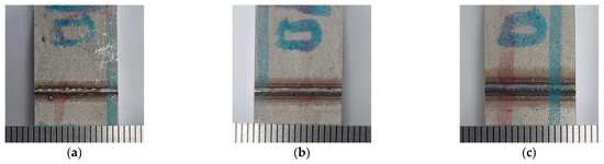
Figure 8.
Visual test for surface bead for welded specimen. (a) P: 3 kW, S:1 m/min, d: 0 mm, (b) P: 4 kW, S: 1 m/min, d: 0 mm, (c) P: 5kW, S: 1 m/min, d: 0 mm.
3. Development Method and Prediction Model
3.1. Global Regression Model
To develop a prediction model using global regression analysis, it is first important to grasp the relationship between the input and output variables. Of these variables, variables that affect other variables are generally called independent variables. A receiving variable is defined as a dependent variable. Regression analysis is a statistical analysis method that assumes a certain mathematical model to estimate the functional relationship between these independent variables and dependent variables, and estimates the model from the measured data. In this paper, the laser power, welding speed, and defocusing were selected as the input variables for the development of a mathematical model using regression analysis. If the bead geometry (penetration depth, bead height, area ratio) is selected as a dependent variable, the relationship between the variables can be expressed using the following Equation (1).
For a linear model (1st order model), the dependent variable can be calculated using a linear combination of independent variables, as shown in Equation (2) below.
A curvilinear (2nd order model) model is expressed in a different form. The function relationship between the input and output variables is the same as shown in Equation (1). When the predictive ability of the linear and curvilinear models is considered, the predicted values of the bead height, penetration depth, and area ratio can be derived. Assuming there is a relationship, it can be expressed in the form of a quadratic regression model as shown in Equation (3).
In this study, since the number of input variables is three, Equation (3) can be expanded as shown in (4), where is an estimate of the output variable (bead height, penetration depth, area ratio), and is the coded unit of input variables (laser power, welding speed, and defocusing). , , and represent the least square estimators of , , and , respectively, and represents the error. The tool used for mathematical model development is Minitab, and the linear regression equations are shown in (5) to (7).
The regression coefficient and the quadratic regression model developed for the dependent variable using Equation (4) can be expressed as in Equations (8)–(10).
Equations (5)–(7) are linear prediction models and Equations (8)–(10) are curvilinear models. is the predicted value of bead height, is the penetration depth, and is the area ratio.
3.2. Local Regression Model
To improve the performance of the prediction model such as bead height, penetration, and area ratio, the prediction performance can be improved through the screening of independent terms. This can be achieved by grasping the influence of individual factors or interactions of factors on the response value. There are three methods. The first is to analyze the coefficients obtained by the test statistics [24]. The second is to compare the relative magnitudes of the effects through normal probability and palette charts [25], and evaluate the degree of influence on the response values through a statistical analysis. The third is to determine influence by visualizing the main effect and mutual effects [26]. In this study, the independent effects and mutual influences of each independent variable were analyzed using the first method and screened for the insignificant factors based on the significant p-value [27]. Table 5, Table 6 and Table 7 are the test statistics for the bead height, penetration depth, and area ratio.
Table 5.
Analysis of variance of global regression model for bead height (.
Table 6.
Analysis of variance of global regression model for penetration depth (
Table 7.
Analysis of variance of global regression model for area ratio (
The p-value refers to the probability value of obtaining the test statistic as a sparse or extreme value from the zero hypothesis of true or false set by the researcher. The lower the calculated p-value, the stronger the evidence to reject the null hypothesis in the sample data. All p-values obtained from the parameter test have a uniform distribution within the range between 0 and 1 in any zero hypothesis. In this study, we tried to secure 80% of probability significance by setting the maximum limit of significance of the p-value to 0.2. The statistical significance of general industrial engineering is based on 0.2, which is determined by the level of demand of the user′s predictive model. As shown in the table, the effect of the relevant factors on the outcome was determined to be a significant factor when the degree of influence was less than 0.2, and as a non-significant factor when the degree of influence was over 0.2, based on the p-value. p-value analysis was used to determine the independence and interaction influence of each variable. As shown in Table 5, the p-values of the main, square, and interaction of the model were 0.001, 0.002, and 0.093, respectively, and the influence on the width of the bead was meaningfully confirmed. In addition, when analyzing each term of the model separately, the interaction between the square of the laser power () term, the welding speed () term, the square of the welding speed () term, the laser power () and the defocusing () () term was found to have a p-value of less than 0.2.
In the analysis of variance of the penetration depth, it was confirmed that the p-value was 0.001, which is a very significant factor for the independent welding speed () and defocusing (). The square terms such as the welding speed () and the defocusing () were also significant. Among the interactions, the interaction () of the laser output () and the welding speed () was influential.
With regard to the area ratio, the squared terms have a large influence on the area ratio and are improved to a significant term. The p-values of the square of the laser output (), the welding speed (), and the defocusing () were 0.035, 0.122, and 0.001, respectively.
Other terms can be identified as meaningless terms with a p-value greater than 0.2. The modified global regression model was developed by eliminating meaningless terms and performing regression analysis again. Equations (11)–(13) below show the modified global regression model.
4. Results and Discussions
4.1. Evaluation of Predictive Performance
In this study, to estimate the performance of the prediction developed using various methods, the sum of the square error (SEE), R-square (, and the standard error (SE) were calculated as expressed in Equations (14) and (15).
The standard error of the evaluation is also called the root mean square error. As a lower value of standard error of the estimate indicates a better fit, it is a good measure of how accurately the model predicts the response. It is also the most important criterion for fit if the main purpose of the model is accuracy of prediction. Moreover, the most important figures here are the and the adjusted-. is calculated as the degree to which the dependent variable is explained by the regression line. In other words, it is a number that shows how well independent variables describe dependent variables. The determination factor is the ratio of the section described by X (welding parameter), which is the overall variable Y of the sub-measure (experimental result). Because the numerator and denominator are nearly identical, the value can be adjacent to 1 if the outcome of each case is similar to the regression value. In addition, the coefficient of determination refers to the ratio, and the square root thereof is the absolute value of the correlation between the dependent variable and the independent variable, and thus has a range of 0 ≤ ≤ 1. The adjusted- is used in a different sense. represents the magnitude of the explanatory power describing the dependent variable, the is generally larger as the independent variable increases in a multiple regression analysis. However, adding the independent variables to raise is contrary to the principle of parsimony, an important principle of regression analysis. The principle of parsimony is that the dependent variable should be described and expressed in as few meaningful variables as possible. Therefore, in order to efficiently explain the dependent variable, only the indispensable independent variables should be included. In addition, since the use of too many independent variables increases the multicollinearity, it is necessary to correct (adjust) the effect of the number of explanatory variables used in the multiple regression model to the decision coefficients. In summary, the adjusted explains the extent to which the dependent variable, taking into account the number of explanatory variables (independent variables), is described. Therefore, it is not necessary to report the adjusted- when a simple regression analysis (one independent variable) is run. It is, however, better to report the adjusted- when a multiple regression analysis (two or more independent variables) is run.
4.2. Global Regression Model
Analysis variance tests were performed to evaluate the performance of the developed global regression model. Analysis variance tests results for the global regression model are shown in Table 8. For the bead height, the value of the linear model was 40.6 and the value of the curvilinear model was 38.7. For penetration depth, the value of the linear model was 52.6 and the value of the curvilinear model was 47.67. For the area ratio, the value of the linear model was 1.9 and the value of the nonlinear model was 43.7. As the order of the prediction model increases, the regression performance increases, and the standard error also decreases. The value of the bead height and area ratio are less than 80%. The standard error of the bead height was 0.1522, which corresponds to the absolute value of the average height (0.159). It was also confirmed that the value of the area ratio was less than 50% and the prediction performance was extremely low. But for the penetration depth, the predictive performance of the curvilinear model was of 83.4% and the standard error was 0.7889, which is about 15% of the average penetration depth (5.09 mm). Bead geometry errors of 15% in the welding process can be evaluated as excellent. To verify the developed equations, the developed linear equations were compared with the experimental data.
Table 8.
Analysis variance tests for global regression model.
Figure 9 compares measured bead geometry and predicted geometry for bead height , penetration depth (), and area ratio (). The diagonal line of the graph is used as a criterion for judging whether or not the predictive performance is accurate. The closer the value is to the diagonal line, the lower the difference between the measured values and the calculated values. In each graph, the predictions based on the first order global regression equation and the second order global regression equation coexist. SEE represents the average range of the errors indicated by the dotted line. It can be confirmed that the penetration depth is close to the diagonal line. This indicates excellent predictive ability. Through the first and second order global regression, the accuracy of penetration depth predictions model is high. However, the bead height and area ratio are distributed widely away from the diagonal line. This indicates that the bead height and area ratio are difficult to predict through the first and second order global regression.
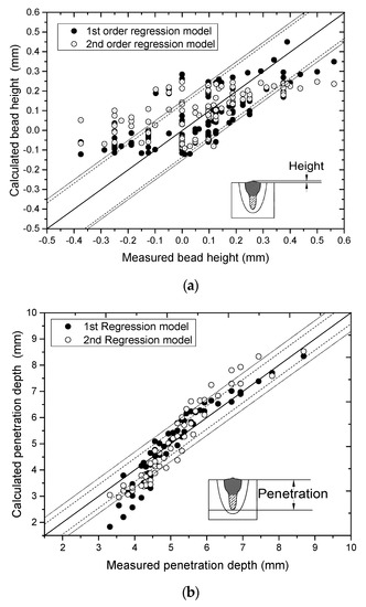
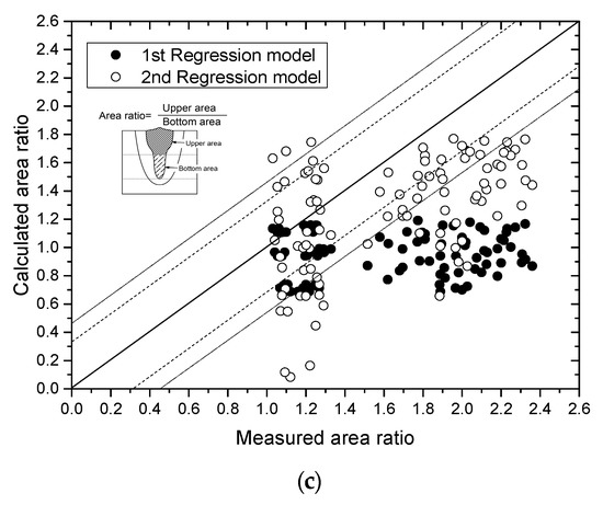
Figure 9.
Comparisons between measured and predicted for 1st order regression model and 2nd regression model: (a) bead height, (b) penetration depth, and (c) area ratio.
4.3. Modified Global Regression Model
To evaluate the performance of the above model, the same analysis variance tests were performed as in previous tests. As can be seen from Table 9 below, for the bead height, was 54.8, of the penetration depth was 84.2, and of the area ratio was 42.5. The maximum measurement value of the bead height was about 1 mm, and it can be confirmed that an error of about 0.7832 mm occurred. The standard error of the penetration depth was 0.4925mm, which was judged to be a small error considering that the maximum penetration depth was 8 mm. For the predicted model of the area ratio, the standard error was close to 0.40, the maximum area ratio measured was 2.3, and 0.4 had a very large range of error. Figure 10 shows comparisons of 100 actual experimental results by applying the modified prediction model.
Table 9.
Analysis variance tests for modified regression model.
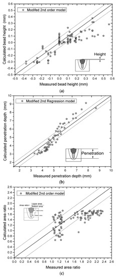
Figure 10.
Prediction performance of the modified global regression model for area ratio: (a) bead height, (b) penetration depth, and (c) area ratio.
The diagonal lines of Figure 10 show the line in which the measured value and the predicted value are matched by the experiment, and the dotted line represents the SSE of each model. As can be seen from Figure 10a, the penetration depth was similar to the actual measured value and the predicted results. Other than the bead height and area ratio, there are two types of variance. The difference between the measured value and the calculated value is large, as shown in Figure 10a,b.
However, the of the bead height and penetration depth in the unmodified curvilinear global regression model was 52.6 and 83.4 (see Table 8 and Table 9), and the values in the modified regression model were revised to 54.8 and 84.2, respectively. Moreover, the predicted performance was improved compared to that of the unmodified model.
For the area ratio, in which the abovementioned two types of dispersion appear, global regression analysis, which analyzes all data at one time, confirmed that there is a prediction limit when one model is used for all cases. This is because the result is confirmed to form two groups, as shown in Figure 10c. To overcome this problem, cluster analysis was applied to form a cluster of input-output variables, and it was necessary to develop a prediction model for the relationship of formed clusters.
In this study, to evaluate the performance of the predictive model, normality evaluation was performed on the difference between the predicted and actual results. Figure 11 shows the results of normality analysis for the residuals of the finally developed regression model. For normality analysis, the Ryan-Joiner normality test was used. This test evaluates normality by calculating the correlation between the data and the normal score of the data. If the correlation coefficient is close to 1, the population is more likely to be normally distributed. The Ryan-Joiner statistic measures the degree of this correlation. If this statistic is less than the appropriate threshold, you reject the null hypothesis that the population is normally distributed. This test is similar to the Shapiro–Wilk normality test.
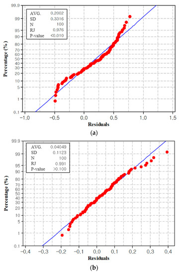
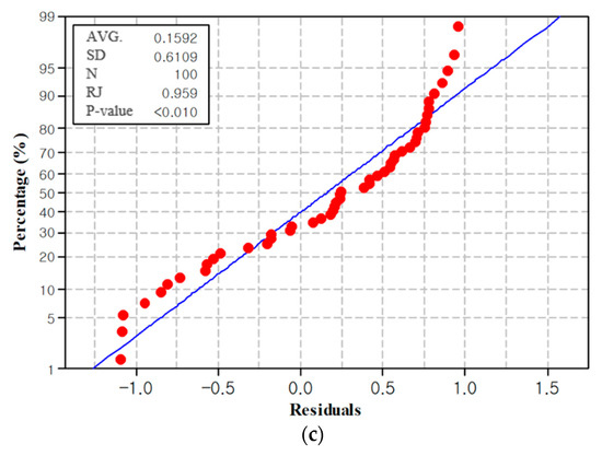
Figure 11.
Normality of the residuals distribution: (a) bead height, (b) penetration depth, (c) area ratio.
To determine whether your data do not follow a normal distribution, compare the p-value to the significance level. Usually, a significance level of 0.05 is appropriate. A significance level of 0.05 indicates that even if the data do not follow a normal distribution, there is a 5% or less risk of the data coming to an incorrect conclusion. Figure 11a,c shows the normality of bead height and area ratio. The p-value of the residual of the predictive model for bead height and area ratio was less than 0.010. It can be concluded that the residuals of the predictive model do not follow a normal distribution. In other words, there is a high probability of not following the normal distribution. However, for the penetration depth shown in Figure 11b, the p-value was greater than 0.1. If the p-value is greater than the significance level, you cannot reject the null hypothesis. There is not enough evidence to conclude that the data do not follow a normal distribution.
5. Conclusions
In this study, a global regression model and a modified regression model were developed to predict the bead shape of the laser welding part of 9% nickel steel. Both models were developed to predict bead height, penetration depth, and melt ratio, and a modified regression model was developed to improve prediction performance. The findings of the research can be summarized as follows.
- (1)
- To apply the laser process of 9% nickel steel, welding was performed by setting welding power, welding speed, and defocusing as input variables using a 5 kw class laser heat source. The bead shape was observed by selecting the bead height, penetration depth, and melting ratio as output variables. It was confirmed that under all conditions, a narrow and deep weld representing the characteristics of the laser weld was formed.
- (2)
- BOP laser welding experiments were performed 100 times using 9% nickel steel, and a global regression model was developed using 100 bead shape data. To improve the predictive performance of the global regression model, which is generally used as a predictive model, a modified global regression model was developed by applying a variable elimination method according to influence using a statistical analysis method.
- (3)
- Analysis variance tests were performed to evaluate the performance of the developed global regression model and modified regression model. The prediction performance was performed using the coefficient of determination (), and the curvilinear model of the global regression model was evaluated to have better prediction performance than the linear model. For bead height, the coefficient of determination of the linear model was 40.6, and that of the curvilinear model was evaluated as 52.6, and neither model achieved excellent performance. For the penetration depth, the coefficient of determination of the linear model was 75.3 and that of the curvilinear model was evaluated as 83.4, and the curvilinear model showed excellent predictive performance. For the area ratio, the coefficient of determination of the linear model was 1.9, which was so poor that the predictive performance could not be evaluated, and the coefficient of determination of the curvilinear model was evaluated as 43.7.
- (4)
- Through evaluating the predictive performance of the modified regression model developed to improve the predictive performance of the global regression model′s curvilinear model, it was confirmed that the predictive performance for bead height and penetration depth were improved by about 1.0% and 0.8%, respectively. However, the predictive performance for area ratio decreased by 1.2%. Global regression and modified regression can predict the bead height and penetration depth, but it is not possible to predict the area ratio. To predict the area ratio, model development using a new analysis method is expected in the future.
- (5)
- The performance of the model was further evaluated indirectly through the verification of the residual normality of the prediction result and the actual value, and it was confirmed that the penetration depth followed the null hypothesis and the result had a normal distribution. However, in the case of bead height and area ratio, an alternative hypothesis was established, confirming that the normal distribution was not followed.
Author Contributions
Methodology, J.K. (Jisun kim); Formal analysis, J.K. (Jisun kim) and J.K. (Jaewoong Kim); software, C.P., resources, J.K. (Jaewoong Kim); writing—original draft, J.K. (Jisun kim); validation, visualization, writing—review and editing, C.P. and K.C.; conceptualization, supervision, investigation, K.C. All authors have read and agreed to the published version of the manuscript.
Funding
This research was financially supported by the Korea Institute of Industrial Technology (KITECH) through the Research and Development “The dynamic parameter control based smart welding system module development for the complete joint penetration weld” (PEH21035).
Data Availability Statement
The data presented in this study are available on request from the corresponding author. The data is private property of Korea Institute of Industrial Technology and is not publicly available.
Conflicts of Interest
The authors declare no conflict of interest.
References
- Schinas, O.; Butler, M. Feasibility and commercial considerations of LNG-fueled ships. Ocean Eng. 2016, 122, 84–96. [Google Scholar] [CrossRef]
- Yoo, B.Y. Economic assessment of liquefied natural gas (LNG) as a marine fuel for CO2 carriers compared to marine gas oil (MGO). Energy 2017, 121, 772–780. [Google Scholar] [CrossRef]
- Thomson, H.; Corbett, J.J.; Winebrake, J.J. Natural gas as a marine fuel. Energy Policy 2015, 87, 153–167. [Google Scholar] [CrossRef]
- Kim, B.E.; Park, J.Y.; Lee, J.S.; Kim, M.H. Study on the Initial Design of an LNG Fuel Tank using 9 wt.% Nickel Steel for Ships and Performance Evaluation of the Welded Joint. J. Weld. Join. 2019, 37, 555–563. [Google Scholar] [CrossRef]
- Na, K.B.; Lee, C.I.; Park, J.H.; Cho, S.M. A Comparison of Hot Cracking in GTAW and FCAW by Applying Alloy 625 Filler Materials of 9% Ni Steel. J. Weld. Join. 2019, 37, 357–362. [Google Scholar] [CrossRef]
- Ruan, X.; Zhou, Q.; Shu, L.; Hu, J.; Cao, L. Accurate Prediction of the Weld Bead Characteristic in Laser Keyhole Welding Based on the Stochastic Kriging Model. Metals 2018, 8, 486. [Google Scholar] [CrossRef]
- Chang, B.; Yuan, Z.; Cheng, H.; Li, H.; Du, D.; Shan, J. A Study on the Influences of Welding Position on the Keyhole and Molten Pool Behavior in Laser Welding of a Titanium Alloy. Metals 2019, 9, 1082. [Google Scholar] [CrossRef]
- Zhang, M.; Zhou, Y.; Huang, C.; Chu, Q.; Zhang, W.; Li, J. Simulation of Temperature Distribution and Microstructure Evolution in the Molten Pool of GTAW Ti-6Al-4V. Alloy. Mater. 2018, 11, 2288. [Google Scholar] [CrossRef]
- Xue, X.; Pereira, A.; Amorim, J.; Liao, J. Effects of Pulsed Nd:YAG Laser Welding Parameters on Penetration and Microstructure Characterization of a DP1000 Steel Butt Joint. Metals 2017, 7, 292. [Google Scholar] [CrossRef]
- Tomasz, K. Heat Source Models in Numerical Simulations of Laser Welding. J. Mater. 2020, 13, 2653. [Google Scholar]
- Pańcikiewicz, K.; Świerczyńska, A.; Hućko, P.; Tumidajewicz, M. Laser Dissimilar Welding of AISI 430F and AISI 304 Stainless Steels. J. Mater. 2020, 13, 4540. [Google Scholar] [CrossRef]
- Landowski, M.; Swierczyńska, A.; Rogalski, G.; Fydrych, D. Autogenous Fiber Laser Welding of 316L Austenitic and 2304 Lean Duplex Stainless Steels. J. Mater. 2020, 13, 2930. [Google Scholar] [CrossRef]
- Kim, J.; Kim, J. Laser Welding of ASTM A553-1 (9% Nickel Steel) (PART II: Comparison of Mechanical Properties with FCAW). Metals 2020, 10, 999. [Google Scholar] [CrossRef]
- Schneller, W.; Leitner, M.; Springer, S.; Grün, F.; Taschauer, M. Effect of HIP Treatment on Microstructure and Fatigue Strength of Selectively Laser Melted AlSi10Mg. J. Manuf. Mater. Process. 2019, 3, 16. [Google Scholar] [CrossRef]
- Sommer, N.; Lehto, J.M.; Völkers, S.; Böhm, S. Laser Welding of Grey Cast Iron with Spheroidal Graphite-Influence of Process Parameters on Crack Formation and Hardness. Metals 2021, 11, 532. [Google Scholar] [CrossRef]
- Wang, W. The Great Minds of Carbon Equivalent (Part lll: The Evolution of Carbon Equivalent Equations); Technical Report of EWI (Edison welding institute): Columbus, OH, USA, 2016. [Google Scholar]
- Asif, K.; Zhang, L.; Derrible, S.; Indacochea, J.E.; Ozenvin, D.; Ziebart, B. Machine learning model to predict welding quality using air-coupled acoustic emission and weld inputs. J. Intell. Manuf. 2020. [Google Scholar] [CrossRef]
- Lee, H.T.; Kim, H.G.; Kim, G.G.; Shin, S.B. A study on the prediction of welding distortion of 9% Ni steel for the offshore LNG storage tank. In Proceedings of the Sixteenth International Offshore and Polar Engineering Conference, Lisbon, Portugal, 1–6 July 2007. [Google Scholar]
- Park, M.H.; Kim, J.; Pyo, C.; Son, J.S.; Kim, J. A Study on the Algorithm of Quality Evaluation for Fiber Laser Welding Process of ASTM A553-1 (9% Nickel Steel) Using Determination of Solidification Crack Susceptibility. J. Mater. 2020, 13, 5617. [Google Scholar] [CrossRef] [PubMed]
- Piekarska, W.; Dorota, G.K. Prediction of structure and mechanical properties of welded joints using analytical methods. Procedia Eng. 2016, 136, 82–87. [Google Scholar] [CrossRef][Green Version]
- Zhang, M.; Tang, K.; Zhang, J.; Mao, C.; Hu, Y.; Chen, G. Effects of processing parameters on underfill defects in deep penetration laser welding of thick plates. Int. J. Adv. Manuf. Technol. 2018, 96, 491–501. [Google Scholar] [CrossRef]
- Unt, A.; Poutiainen, I.; Grünenwald, S.; Sokolov, M.; Salminen, A. High Power Fiber Laser Welding of Single Sided T-Joint on Shipbuilding Steel with Different Processing Setups. Appl. Sci. 2017, 7, 1276. [Google Scholar] [CrossRef]
- Matsuoka, S.; Okamoto, Y.; Okada, A. Influence of Weld Bead Ggeometry on Thermal Deformation in Laser Micro-Welding. Procedia CIRP 2013, 6, 492–497. [Google Scholar] [CrossRef]
- Park, H.S.; Kim, T.H.; Lee, S.H. Optimization of Welding Parameters for Resistance Spot Welding of TRIP Steel using Response Surface Metho dology. J. Korean Weld. Join. Soc. 2003, 21, 76–81. [Google Scholar]
- Park, H.J.; Kang, M.J.; Choi, B.G.; Lee, S.H. Welding Parameters Optimization of Pleated Type Metallic Filter Using Response Surface Methodology. In Proceedings of the Korean Welding and Joining Society Conference, Jeju, Korea, 2–5 March 2004; pp. 39–41. [Google Scholar]
- Son, C.K.; Oh, S.J.; Lee, G.J. Analysis of the Relationship among Ambient Conditions and Ice Accretion Shapes by Employing Self-Organization Map and ANOVA. In Proceedings of the Korean Society for Aeronautical & Space Sciences Conference proceeding, Seoul, Korea, 18 November 2011; pp. 91–96. [Google Scholar]
- Laszlo, Z.G.; Pierre, D.V. Perturbations on the Uniform Distribution of P-values can Lead to Misleading Inferences from Null-Hypothesis Testing. J. Trends Neurosci. Educ. 2017, 8, 18–27. [Google Scholar]
Publisher’s Note: MDPI stays neutral with regard to jurisdictional claims in published maps and institutional affiliations. |
© 2021 by the authors. Licensee MDPI, Basel, Switzerland. This article is an open access article distributed under the terms and conditions of the Creative Commons Attribution (CC BY) license (https://creativecommons.org/licenses/by/4.0/).