1. Introduction
Membrane computing [
1,
2] is an interdisciplinary research area in the intersection of computer science and cellular biology mainly [
3], but also with many other fields such as engineering, neuroscience, systems biology, chemistry, etc. The aim is to study computational devices called P systems, taking inspiration from how living cells process information. Spiking neural P (SNP) systems [
4] are a type of P system composed of a directed graph inspired by how neurons are interconnected by axons and synapses in the brain. Neurons communicate through spikes, and the time difference between them plays an important role in the computation. Therefore, this model belongs to the known third generation of artificial neural networks, i.e., based on spikes.
Aside from computing numbers, SNP systems can also compute strings, and hence, languages. More general ways to provide the input or receive the output include the use of spike trains, i.e., a stream or sequence of spikes entering or leaving the system. Further results and details on computability, complexity, and applications of spiking neural P systems are detailed in [
5,
6,
7], a dedicated chapter in the Handbook in [
8], and an extensive bibliography until February 2016 in [
9]. Moreover, there is a wide range of SNP system variants: with delays, with weights [
10], with astrocytes [
11], with anti-spikes [
12], dendrites [
13], rules on synapses [
14], scheduled synapses [
15], stochastic firing [
16], numerical [
17], etc.
The research on applications and variants of SNP systems has required the development of simulators. The simulation of SNP systems was initially carried out through sequential simulators such as pLinguaCore [
18]. In 2010, a matrix representation of SNP systems was introduced [
19]. Since then, most simulation algorithms are based on matrices and vector representations, and consists of a set of linear algebra operations. This way, parallel simulators can be efficiently implemented, since matrix-vector multiplications are easy to parallelize. Moreover, there are efficient algebra libraries that can be used out-of-the-box, although they have not been explored yet for this purpose. For instance, GPUs are parallel devices optimized for certain matrix operations [
20], and can handle matrix operations efficiently. We can say, without loss of generality, that these matrix representations of SNP systems fit well to the highly parallel architecture of these devices. This have been harnessed already by introducing CuSNP, a set of simulators for SNP systems implemented with CUDA [
21,
22,
23,
24]. Simulators for specific solutions have been also defined in the literature [
5,
25]. Moreover, this is not unique for SNP systems, many simulators for other P system variants have been accelerated on GPUs [
26,
27,
28].
However, this matrix representation can be sparse (i.e., having a majority of zero values) because the directed graph of SNP systems is not usually fully connected. A first approach to tackle this problem was presented in [
29], where some of the ideas described in this work were described. Following these ideas, in [
30], the transition matrix was split to reduce the memory footprint of the SNP representation. In many disciplines, sparse vector-matrix operations are very usual, and hence, many solutions based on compressed implementations have been proposed in the literature [
31].
In this paper, we introduce compressed representations for the simulation of SNP systems based on sparse vector-matrix operations. First, we provide two approaches to compress the transition matrix for the simulation of SNP systems with static graph. Second, we extend these algorithms and data structures for SNP systems with dynamic graphs (division, budding, and plasticity). Finally, we make a complexity analysis and comparison of the algorithms to draw some conclusions.
The paper is structured as follows:
Section 2 provides required concepts for the methods and algorithms here defined;
Section 3 defines the designs of the representations;
Section 4 contains the detailed algorithms based on the compressed representations;
Section 5 shows the results on complexity analyses of the algorithms;
Section 6 provides final conclusions, remarks, and plans of future work.
2. Preliminaries
In this section we briefly introduce the concepts employed in this work. Firstly, we define the standard model of spiking neural P systems and three variants. Second, a matrix-based simulation algorithm for this model is revisited. Third, the fundamentals of compressed formats for sparse matrix-vector operations are given.
2.1. Spiking Neural P Systems
Let us first formally introduce the definition of spiking neural P system. This model was first introduced in [
4].
Definition 1. A spiking neural P system
of degree is a tuplewhere: is the singleton alphabet (a is called spike);
represents the arcs of a directed graph whose nodes are ;
are neurons of the formwhere: - –
is the initial number of spikes within neuron labeled by i; and
- –
is a finite set of rules associated to neuron labeled by i, of one of the following forms:
- (1)
, being E a regular expression over , (firing rules);
- (2)
for some , with the restriction that for each rule of type of type from , we have (forgetting rules).
such that , for any .
A spiking neural P system of degree can be viewed as a set of q neurons interconnected by the arcs of a directed graph , called synapse graph. There is a distinguished neuron label , called output neuron (), which communicates with the environment.
If a neuron contains k spikes at an instant t, and , then the rule can be applied. By the application of that rule, c spikes are removed from neuron and the neuron fires producing p spikes immediately. Thus, each neuron such that receives p spikes. For , the output neuron , the spikes are sent to the environment.
The rules of type are forgetting rules, and they are applied as follows: If neuron contains exactly s spikes, then the rule from can be applied. By the application of this rule all s spikes are removed from .
In spiking neural P systems, a global clock is assumed, marking the time for the whole system. Only one rule can be executed in each neuron at step t. As models of computation, spiking neural P systems are Turing complete, i.e., as powerful as Turing machines. On one hand, a common way to introduce the input (instance of the problem to solve) to the system is to encode it into some or all of the initial spikes ’s (inside each neuron i). On the other hand, a common way to obtain the output is by observing neuron : either by getting the interval where sent its first two spikes at times and (we say n is computed or generated by the system), or by counting all the spikes sent by to the environment until the system halts.
For the rest of the paper, we call this model spiking neural P systems with static structure, or just static SNP, given that the graph associated with it does not change along the computation. Next, we briefly introduce and focus on three variants with a dynamic graph: division, budding, and plasticity. A broader explanation of them and more variants are provided at [
32,
33,
34,
35].
Finally, let us introduce some notations and definitions:
: for a neuron , the presynapses of this neuron is .
: for a neuron , the out degree of this neuron is: .
: for a neuron , the insynapses of this neuron is .
: for a neuron , the in degree of this neuron is: .
2.1.1. Spiking Neural P Systems with Budding Rules
Based on the idea of neuronal budding, where a cell is divided into two new cells, we can abstract it to budding rules. In this process, the new neurons can differ in some aspects: their connections, contents, and shape. A budding rule has the following form:
where
E is a regular expression and
.
If a neuron contains s spikes, , and there is no neuron such that there exists a synapse in the system, then the rule is enabled and it can be executed. A new neuron is created, and both neurons and are empty after the execution of the rule. This neuron keeps all the synapses that were going in, and this inherits all the synapses that were going out of in the previous configuration. There is also a synapse between neurons and , and the rest of synapses of are given to the neuron depending on the synapses of .
2.1.2. Spiking Neural P Systems with Division Rules
Inspired by the process of
mitosis, division rules have been widely used within the field of
membrane computing. In SNP systems, a division rule can be defined as follows:
where
E is a regular expression and
.
If a neuron contains s spikes, , and there is no neuron such that the synapse or exists in the system, , then the rule is enabled and it can be executed. Neuron is then divided into two new cells, and . The new cells are empty at the time of their creation. The new neurons keep the synapses previously associated to the original neuron , that is, if there was a synapse from to , then a new synapse from to and a new one to are created, and if there was a synapse from to , then a new synapse from to and a new one from to are created. The rest of synapses of and are given by the ones defined in .
2.1.3. Spiking Neural P Systems with Plasticity Rules
It is known that new synapses can be created in the brain thanks to the process of
synaptogenesis. We can recreate this process in the framework of spiking neural P systems defining
plasticity rules in the following form:
where
E is a regular expression,
,
,
and
(a.k.a. neuron set). Recall that
is the set of presynapses of neuron
.
If a neuron contains s spikes, , then the rule is enabled and can be executed. The rule consumes c spikes and, depending on the value of , it performs one of the following:
If and , or if and , then there is nothing more to do.
If and , deterministically create a synapse to every , . Otherwise, if , then non-deterministically select k neurons in and create one synapse to each selected neuron.
If and , deterministically delete all synapses in . Otherwise, if , then non-deterministically select k neurons in and delete each synapse to the selected neurons.
If , create (respectively, delete) synapses at time t and then delete (resp., create) synapses at time . Even when this rule is applied, neurons are still open, that is, they can continue receiving spikes.
Let us notice that if, for some , we apply a plasticity rule with , when a synapse is created, a spike is sent from to the neuron that has been connected. That is, when attaches to through this method, we have immediately transferring one spike to .
2.2. Matrix Representation for SNP Systems
Usually, parallel, P system simulators make use of
ad-hoc representations, tailored for a certain variant [
26,
27,
28]. In order to ease the simulation of static SNP system and its deployment to parallel environments, a matrix representation was introduced [
19]. By using a set of algebraic operations, it is possible to reproduce the transitions of a computation. Although the baseline representation only involves SNP systems without delays and static structure, many extensions have followed such as for enabling delays [
21,
22], handling non-determinism [
24], plasticity rules [
36], rules on synapses [
37], and dendrite P systems [
38]. In this section we briefly introduce the definitions for the matrix representation of the basic model of spiking neural P systems without delays, as defined above. We also provide the pseudocode to simulate just one computation of any P system of the variant using this matrix representation. In our notation, we use capital letters for vectors and matrices, and
for accessing values:
is the value at position
i of the vector
V, and
is the value at row
i and column
j of matrix
M.
For an SNP system of degree (q neurons and m rules, where ), we define the following vectors and matrices:
Configuration vector: is the vector containing all spikes in every neuron on the k computation step/time, where denotes the initial configuration; i.e., , for neuron . It contains q elements.
Spiking vector: shows if a rule is going to fire at the transition step k (having value 1) or not (having value 0). Given the non-determinism nature of SNP systems, it would be possible to have a set of valid spiking vectors, which is denoted as . However, for the computation of the next configuration vector, only a spiking vector is used. It contains m elements.
Transition matrix:
is a matrix comprised of
elements given as
In this representation, rows represent rules and columns represent neurons in the spiking transition matrix. Note also that a negative entry corresponds to the consumption of spikes. Thus, it is easy to observe that each row has exactly one negative entry, and each column has at least one negative entry [
19].
Hence, to compute the transition k, it is enough to select a spiking vector from all possibilities and calculate: .
The pseudocode to simulate a computation of an SNP system is as described in Algorithm 1. The selection of valid spiking vectors can be done in different ways, as in [
21,
22]. This returns a set of valid spiking vectors. In this work, we focus on just one computation, but non-determinism can be tackled by maintaining a queue of generated configurations [
24].
| Algorithm 1 MAIN PROCEDURE: simulating one computation for static spiking neural P systems. |
Require: A SNP system of degree , and a limit L of time steps. Ensure: A computation of the system
- 1:
INIT() - 2:
- 3:
repeat - 4:
SPIKING_VECTORS() ▹ Calculate all possible spiking vectors - 5:
GET_ONE_RANDOMLY() ▹ Pick one spiking vector randomly - 6:
▹ Compute next configuration - 7:
- 8:
until ▹ Stop condition: maximum steps or no more applicable rules - 9:
return
|
In this work we focus on compressing the representation, specifically the transition matrix, so the determination of the spiking vector is not affecting these designs. Therefore, we use a straightforward approach and select just one valid spiking vector randomly. The representations here depicted only affect how the computation of the next configuration is done (matrix-vector multiplication at line 6 in Algorithm 1).
2.3. Sparse Matrix-Vector Operations
Algebraic operations have been studied deeply in parallel computing solutions. Specifically, GPU computing provides large speedups when accelerating such kind of operations. This technology allows us to run scientific computations in parallel on the GPU, given that a GPU device typically contains thousands of cores and high memory bandwidth [
39]. However, parallel computing on a GPU has more constraints than on a CPU: threads have to run in an SPMD fashion while accessing data in a coalesced way; that is, best performance is achieved when the execution of threads is synchronized and accessing contiguous data from memory. In fact, GPUs have been employed for P system simulations since the introduction of CUDA.
Matrix computation is a highly optimized operation in CUDA [
40], and there are many efficient libraries for algebra computations like cuBLAS. It is usual that when working with large matrices, these are almost “empty”, or with a majority of zero values. This is known as
sparse matrix, and this downgrades the runtime in two ways: lot of memory is wasted, and lot of operations are redundant.
Given the importance of linear algebra in many computational disciplines, sparse vector-matrix operations (SpMV) have been subject of study in parallel computing (and so, on GPUs). Today there exists many approaches to tackle this problem [
41]. Let us focus on two formats to represent sparse matrices in a compressed way, assuming that threads access rows in parallel:
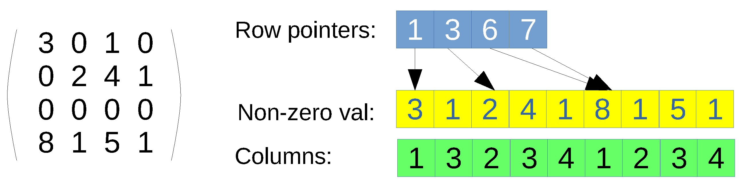
CSR format. Only non-null values are represented by using three arrays: row pointers, non-zero values, and columns (see
Figure 1 for an example). First, the row-pointers array is accessed, which contains a position per row of the original matrix. Each position says the index where the row start in the non-zero values and columns arrays. The non-zero values and the columns arrays can be seen as a single array of pairs, since every entry has to be accessed at the same time. Once a row is indexed, then a loop over the values in that row has to be performed, so that the corresponding column is found, and therefore, the value. If the column is not present, then the value is assumed to be zero, since this data structure contains all non-zero values. The main advantage is that it is a full-compressed format if
, where
and
are the number of non-zero and zero values in the original matrix, respectively. However, the drawbacks is that the search of elements in the non-zero values and columns arrays is not coalesced when using parallelism per row. Moreover, since it is a full-compressed format, there is no room for modifying the values, such as introducing new non-zero values;
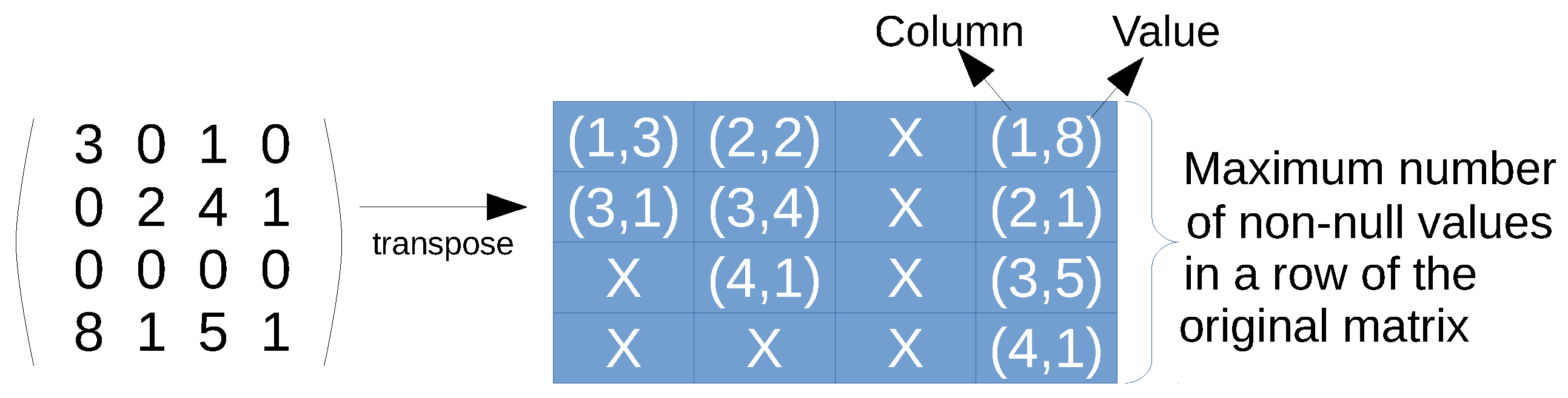
ELL format. This representation aims at increasing the memory coalescing access of threads in CUDA. This is achieved by using a matrix of pairs, containing a trimmed, transposed version of the original matrix (see
Figure 2 for an example). Each column of the ELL matrix is devoted to each row of the matrix, even though the row is empty (all elements are zero). Every element is a pair, where the first position denotes the column and the second is the value, of only the non-zero elements in the corresponding row. However, the size of the matrix is fixed, so the number of columns equals the number of rows of the original matrix, but the number of rows is the maximum length of a row in terms of non-zero values; in other words, the maximum amount of non-zero elements in a row of the original matrix. Rows containing fewer elements pad the difference with null elements. The main advantage of this format is that threads always access the elements of all rows in coalesced way, and the null elements padded by short rows can be utilized to incorporate new data. However, there is a waste of memory, which is worst when the rows are unbalanced in terms of number of zeros.
3. Methods
SNP systems in the literature typically do not contain fully connected graphs. This means that the transition matrix gets very sparse and, therefore, both computing time and memory are wasted. However, further optimizations based on SpMV can be conveyed. In the following subsections we discuss some approaches. Of course, if the graph inherent to an SNP system leads to a compressed transition matrix, then a normal (sparse) format can be employed, because using compressed formats will increase the memory footprint.
In this work, we focus on the basic model of spiking neural P systems without delays as defined above, as well as three variants with dynamic network: budding, division and plasticity. The set of algorithms defined next are designed to take advantage of data parallelism, what is convenient for GPUs and vector co-processors. Their pseudocodes are detailed in
Section 4 of this paper.
In Algorithm 2 we generalize the pseudocode disposed in Algorithm 1 to be able to handle both static and dynamic networks. This way, each variant requires to re-define just some functions from the ones defined for the static SNP system variant using vector and matrices without compression (i.e., sparse representation). In order to understand the algorithms, we will present in this section the main new data structures and their behavior. The detailed pseudocodes are available in
Section 4.
| Algorithm 2 MAIN PROCEDURE: simulating one computation for spiking neural P systems. |
Require: An SNP system of degree , and a limit L of time steps. Ensure: A computation of the system
- 1:
INIT() - 2:
- 3:
repeat - 4:
SPIKING_VECTORS() ▹ Calculate all possible spiking vectors - 5:
GET_ONE_RANDOMLY() ▹ Pick one spiking vector randomly - 6:
COMPUTE_NEXT() ▹ Compute next configuration - 7:
- 8:
until▹ Stop condition: maximum steps or no more applicable rules - 9:
return
|
As a convention, those vectors and matrices using subindex k are dynamic and can change during the simulation time, while those with subindex are constructed at the beginning and are invariant. Capital letters refer to vectors and matrices, and small letters are scalar numbers. A total order over the rules defined in the system is assumed, which is denoted as . For the sake of simplicity, we represent each rule , with , as a tuple , where i is the subindex of the set where belongs (i.e., the neuron where it is contained). Specifically, forgetting rules just have .
For static SNP systems using sparse representation, we use the following vectors and matrices:
Preconditions vector is a vector storing the preconditions of the rules; that is, both the regular expression and the consumed spikes. Initially, , for each .
Neuron-rule map vector is a vector that maps each neuron index with its rules indexes. Specifically, is the index of the first rule in the neuron. Given that rules have been ordered in R as mentioned above, rules belonging to the same neuron have contiguous indexes. Thus, it is enough to store just the first index. In this sense, the first rule in neuron i is and the last one is . In other words, contains elements, and it is initialized as follows: . Specifically, and , for
is the transition tuple, where . If the variant has a dynamic network, the transition matrix needs to be modified. Therefore, we start with . The following algorithms show how they are constructed.
Algorithm 2 can be easily transformed to Algorithm 1 by defining the INIT and COMPUTE_NEXT functions as in Algorithm 3. They work exactly as already specified in
Section 2.2; that is, using the usual vector-matrix multiplication operation to calculate the next configuration vector. We will also detail how the selection of spiking vectors can be done. This is defined in Algorithm 4, and it is based on previous ideas already presented in [
21,
22]. First, SPIKING_VECTORS function calculates the set of all possible spiking vectors by using a recursive function over neuron index
i. It gathers all spiking vectors that can be generated for neurons
and then. If neuron
i contains applicable rules, it populates a spiking vector for each of these rules, and from each of the generated spiking vectors form neurons
. Finally, neuron
i propagates these spiking vectors to the next neuron
.
| Algorithm 3 Functions for static SNP systems with sparse matrix representation. |
- 1:
procedureINIT() - 2:
INIT_NEURON_VECTORS() - 3:
INIT_RULE_MATRICES() - 4:
- 5:
return - 6:
end procedure -
- 7:
procedureINIT_NEURON_VECTORS() - 8:
- 9:
EMPTY_VECTOR(q) - 10:
EMPTY_VECTOR() - 11:
- 12:
for all do - 13:
- 14:
- 15:
- 16:
end for - 17:
return - 18:
end procedure -
- 19:
procedureINIT_RULE_MATRICES() - 20:
- 21:
EMPTY_VECTOR(m) - 22:
EMPTY_MATRIX() - 23:
for all do - 24:
- 25:
- 26:
- 27:
for all do - 28:
- 29:
end for - 30:
end for - 31:
return - 32:
end procedure -
- 33:
procedureCOMPUTE_NEXT() - 34:
- 35:
return - 36:
end procedure
| ▹ Initialize vectors only related to neurons. ▹ Initialize matrices related to rules. ▹ Get information from ▹ Create initial configuration ▹ Create neuron-rule vector ▹ For each neuron ▹ Get info of the neuron from ▹ Initial configuration ▹ Neuron-rule map vector initialization ▹ Get information from ▹ Create preconditions vector ▹ Create transition matrix ▹ For each rule (column). This loop is parallelizable. ▹ Get info of the rule ▹ Store it in precondition vector ▹ Construct transition matrix ▹ For each connected neuron to ▹ Construct transition matrix ▹ Get some content of transition tuple ▹ Only the configuration is updated.
|
| Algorithm 4 Spiking vectors selection with static SNP systems and sparse representation. |
- 1:
procedureSPIKING_VECTORS() - 2:
return COMBINATIONS() - 3:
end procedure -
- 4:
procedureCOMBINATIONS() - 5:
- 6:
- 7:
if then - 8:
return ∅ - 9:
else - 10:
- 11:
COMBINATIONS() - 12:
if then - 13:
EMPTY_VECTOR(m) - 14:
- 15:
else - 16:
- 17:
end if - 18:
for do - 19:
if APPLICABLE() then - 20:
for all do - 21:
- 22:
- 23:
- 24:
end for - 25:
end if - 26:
end for - 27:
if then - 28:
return - 29:
else - 30:
return - 31:
end if - 32:
end if - 33:
end procedure -
- 34:
procedureAPPLICABLE() - 35:
- 36:
- 37:
return - 38:
end procedure -
- 39:
procedureGET_ONE_RANDOMLY() - 40:
Random() - 41:
return -th spiking vector in - 42:
end procedure
| ▹ Start calculating combinations from neuron 1 ▹ With dynamic networks, ▹ Get some content of transition tuple ▹ If neuron i is out of index. ▹ An empty set. ▹ The set for the rest of neurons. ▹ All combinations for rest of neurons. ▹ No spiking vectors yet for rest of neurons ▹ Create an empty spiking vector. ▹ The set to loop over just contains S ▹ There are spiking vectors for rest of neurons ▹ The set to loop over is just ▹ For each rule in neuron i ▹ If rule j is applicable ▹ For each spiking vector, either or empty vector ▹ Create a copy ▹ Mark rule j as applicable ▹ Add it to the solution ▹ If there are no applicable rules ▹ Just propagate combinations ▹ Return calculated combinations ▹ Get some content of transition tuple ▹ Preconditions of the rule ▹ If rule j is applicable in neuron i ▹ Returns just one randomly chosen
|
3.1. Approach with ELL Format
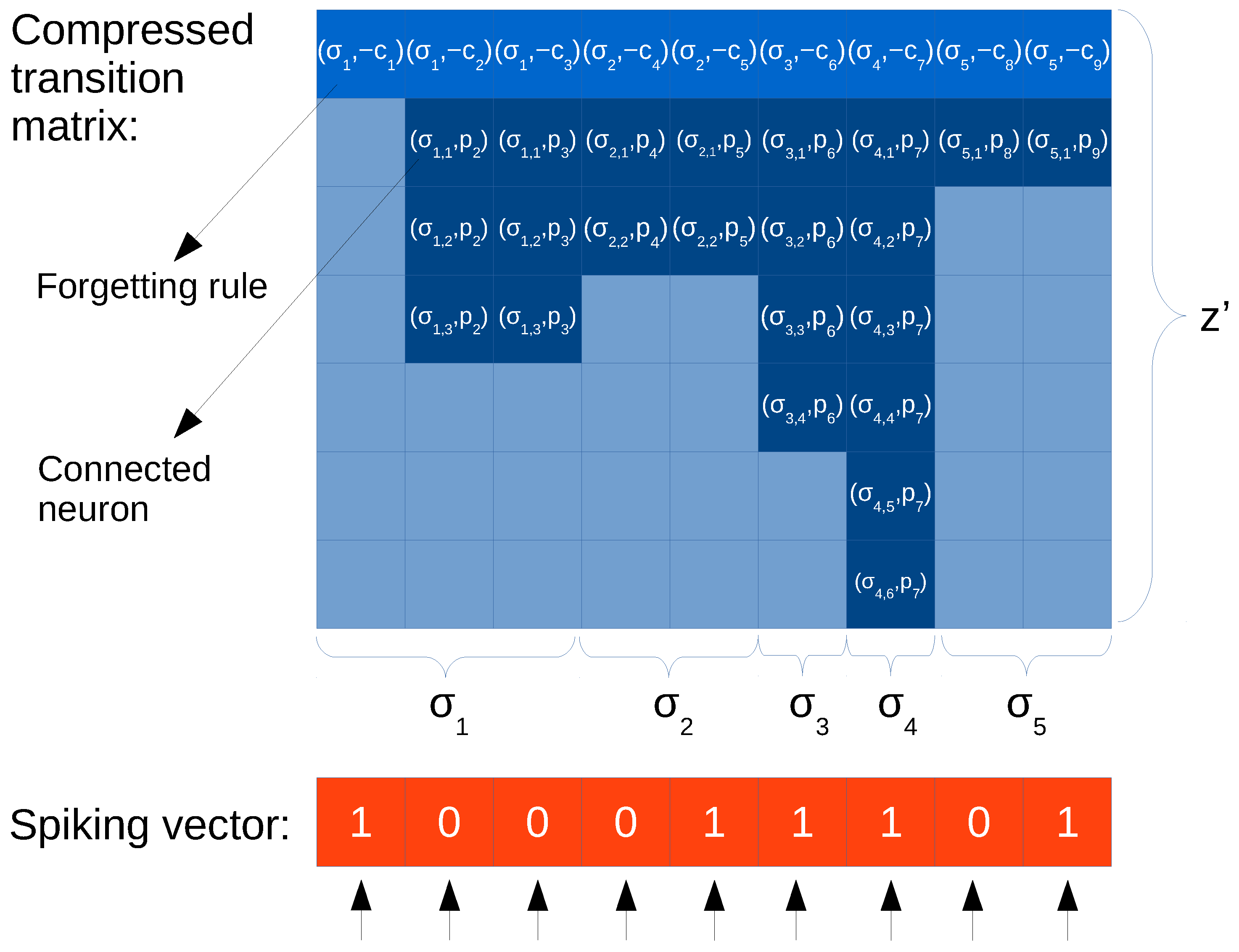
Our first approach to compress the representation of the transition matrix,
, is to use the ELL format (see
Figure 3 for an example). The reason for using ELL and not other compressed formats for sparse matrices (CSR, COO, BSR, …) is to enable extensions for dynamic networks, as seen later. ELL can give some room for modifications without much memory re-allocations, while CSR requires us to modify the whole matrix to add new elements.
ELL format leads to the new compressed matrix . The following aspects have been taken into consideration:
The ELL format represents the transpose of the original matrix, so now rows correspond to neurons and columns to rules. This is convenient for SIMD processors such as GPUs.
The number of rows of
equals the maximum amount of non-zero values in a row of
, denoted by
. It can be shown that
, where
z is the maximum output degree found in the neurons of the SNP system. Specifically,
(see definition in
Section 2.1).
can be derived from the composition of the transition matrix, where row
j devoted for rule
contains the values
for every neuron
i (columns) connected though an output synapse with the neuron where the rule belongs to (i.e.,
), and a value
for consuming the spikes in the neuron the rule belongs to (i.e.,
).
The values inside columns can be sorted, so that the consumption of spikes ( values) are placed at the first row. In this way, if implemented in parallel, all threads can start by doing the same task: consuming spikes.
Every position of
is a pair (as illustrated in
Figure 3), where the first element is a neuron label, and the second is the number of spikes produced (
).
A parallel code can be implemented with this design by assigning a thread to each rule, and so, one per column of the spiking vector and one per column of (rows of the original transition matrix). For the vector-matrix multiplication, it is enough to have a loop of steps at maximum through the columns. In the loop of each column j, the corresponding value in the spiking vector (either 0 or 1) is multiplied to the value in the pair , and added to the neuron id in the configuration vector . In case the SNP network contains hubs (nodes with high amount of input synapses), then we can opt for a parallel reduction per column. Since some threads might write to same positions in the configuration vector at the same time, a solution would be to use atomic adding operations, which are available on devices such as GPUs.
In order to use this representation in Algorithm 2, we only need to re-define functions INIT_RULE_MATRICES and COMPUTE_NEXT from Algorithm 3 (for sparse representation) as shown in Algorithm 5. The rest of functions remain unchanged.
| Algorithm 5 Functions for static SNP systems with ELL-based matrix representation. |
- 1:
procedureINIT_RULE_MATRICES() - 2:
- 3:
EMPTY_VECTOR(m) - 4:
EMPTY_MATRIX() - 5:
for all do - 6:
- 7:
- 8:
- 9:
if then - 10:
- 11:
for all do - 12:
- 13:
- 14:
end for - 15:
end if - 16:
end for - 17:
return - 18:
end procedure - 19:
procedureCOMPUTE_NEXT() - 20:
- 21:
- 22:
for do - 23:
- 24:
repeat - 25:
- 26:
- 27:
- 28:
until - 29:
end for - 30:
return - 31:
end procedure
| ▹ Get information from ▹ Create preconditions vector ▹ Create transition matrix ▹ For each rule (column). This loop is parallelizable. ▹ Get info of the rule ▹ Store it in precondition vector ▹ Only for the first row ▹ Only if is not a forgetting rule ▹k is our iterator, compacting the rows ▹ For each out synapse ▹ Add out neuron and produced spikes ▹ We know that ▹ Create a copy of ▹ Get some content of transition tuple ▹ For each rule (column). This loop is parallelizable. ▹ Get info from transition matrix ▹ Update configuration, if not applicable, ▹ Until reaching an empty value or the maximum
|
3.2. Optimized Approach for Static Networks
If, in general, more than one rule are associated to each neuron, many of the iterations in the main loop in COMPUTE_NEXT function are wasted. Indeed, if the loop is parallelized and each iteration is assigned to a thread, then many of them will be inactive (having a 0 in the spiking vector), causing performance drops such as branch divergence and non-coalesced memory access in GPUs. Moreover, note in
Figure 3 that columns corresponding to rules belonging to the same neuron contain redundant information: the generation of spikes (
) is replicated for all synapses.
Therefore, a more efficient compressed matrix representation can be obtained when maintaining the synapses separated from the rule information. This is called optimized matrix representation, and can be done with the following data structures:
Rule vector,
. By using a CSR-like format (see
Figure 4 for an example), rules of the form
(also forgetting rules are included, assuming
) can be represented by an array storing the values
c and
p in a pair. We can use the already defined neuron-rule map vector
to relate the subset of rules associated to each neuron.
Synapse matrix,
. It is a transposed matrix as with ELL representation (to better fit to SIMD architectures such as GPU devices), but it has a column per neuron
i and a row for every neuron
j such that
(there is a synapse). That is, every element of the matrix corresponds to a synapse (the neuron id) or a null value otherwise. Null values are employed for padding the columns, since the number of rows equals
z (the maximum output degree in the neurons of the SNP system). See
Figure 4 for an example.
Spiking vector is modified, containing only q positions instead of n (i.e., one per neuron), and states which rule is selected.
Note that we replace the transition matrix for a pair with rule vector and synapse matrix: . In order to compute the next configuration, it is enough to loop over the neurons. Then, for each neuron i, we check which rule j is selected, according to the spiking vector at position . This is used to grab the pair from the rule vector, and therefore consume spikes in the neuron i and add spikes in the neurons at the column i of the synapse matrix. The loop over the column can end prematurely if the out degree of neuron i is not z (that is, when encountering a null value). This operation can be easily parallelized by assigning a thread to each column of the synapse matrix (requiring q threads, one per neuron).
In order to use this optimized representation in Algorithm 2, we need to re-define the spiking selection function, since this vector works differently. To do this, it is enough to just modify two lines in the definition of COMBINATIONS function at Algorithm 4, in order to keep the spiking vector with size
q and storing the rule id instead of just 1 or 0 (see
Section 4 for more detail). Moreover, we need to define tailored INIT_RULE_MATRICES and COMPUTE_NEXT functions as shown in Algorithm 6, replacing those from Algorithm 3.
| Algorithm 6 Functions for static SNP systems with optimized compressed matrix representation. |
- 1:
procedureINIT_RULE_MATRICES() - 2:
- 3:
EMPTY_VECTOR(m) - 4:
EMPTY_VECTOR(m) - 5:
for all do - 6:
- 7:
- 8:
- 9:
end for - 10:
EMPTY_MATRIX() - 11:
for do - 12:
- 13:
for all do - 14:
- 15:
- 16:
end for - 17:
end for - 18:
- 19:
return - 20:
end procedure -
- 21:
procedureCOMPUTE_NEXT() - 22:
- 23:
- 24:
- 25:
for do - 26:
- 27:
if then - 28:
- 29:
- 30:
- 31:
while do - 32:
- 33:
- 34:
- 35:
end while - 36:
end if - 37:
end for - 38:
return - 39:
end procedure
| ▹ Get information from ▹ Create preconditions vector ▹ For each rule (column). This loop is parallelizable. ▹ Get info of the rule ▹ Store it in precondition vector ▹ Store it in rule vector ▹ For each neuron (column in synapse matrix) ▹k is our iterator, compacting the rows ▹ For each out synapse ▹ We know that ▹ Create a copy of ▹ Get some content of transition tuple ▹ For each neuron. This loop is parallelizable. ▹ Index of rule to fire in the neuron ▹ Only if there is a rule. ▹ Get rule info ▹ Consume spikes in firing neuron ▹ Next while stops if , i.e., a firing rule ▹ Until an empty value or the maximum ▹ Get connected neuron by a synapse ▹ Produce spikes in connected neuron
|
3.3. Optimized Approach for Dynamic Networks
The optimized compressed matrix representation discussed in
Section 3.2 can be further extended to support rules that modify the network, such as budding, division, or plasticity.
3.3.1. Budding and Division Rules
We start by analyzing how to simulate dynamic SNP systems with budding and division rules. They are supported at the same time in order to unify the pseudocode and also because both kind of rules are usually together in the model.
First of all, the synapse matrix has to be flexible enough to host new neurons. This can be accomplished by allocating a matrix large enough to populate new neurons (probably up to fill the whole memory available). We denote
as the maximum amount of neurons that the simulator is able to support, and
the amount of neurons in a given step
k. The formula to calculate
is in
Section 5. It is important to point out that the simulator needs to differentiate between neuron label and neuron id [
35]. The reason for this separation is that we can have more than one neuron (with different ids) with the same label (and hence, rules).
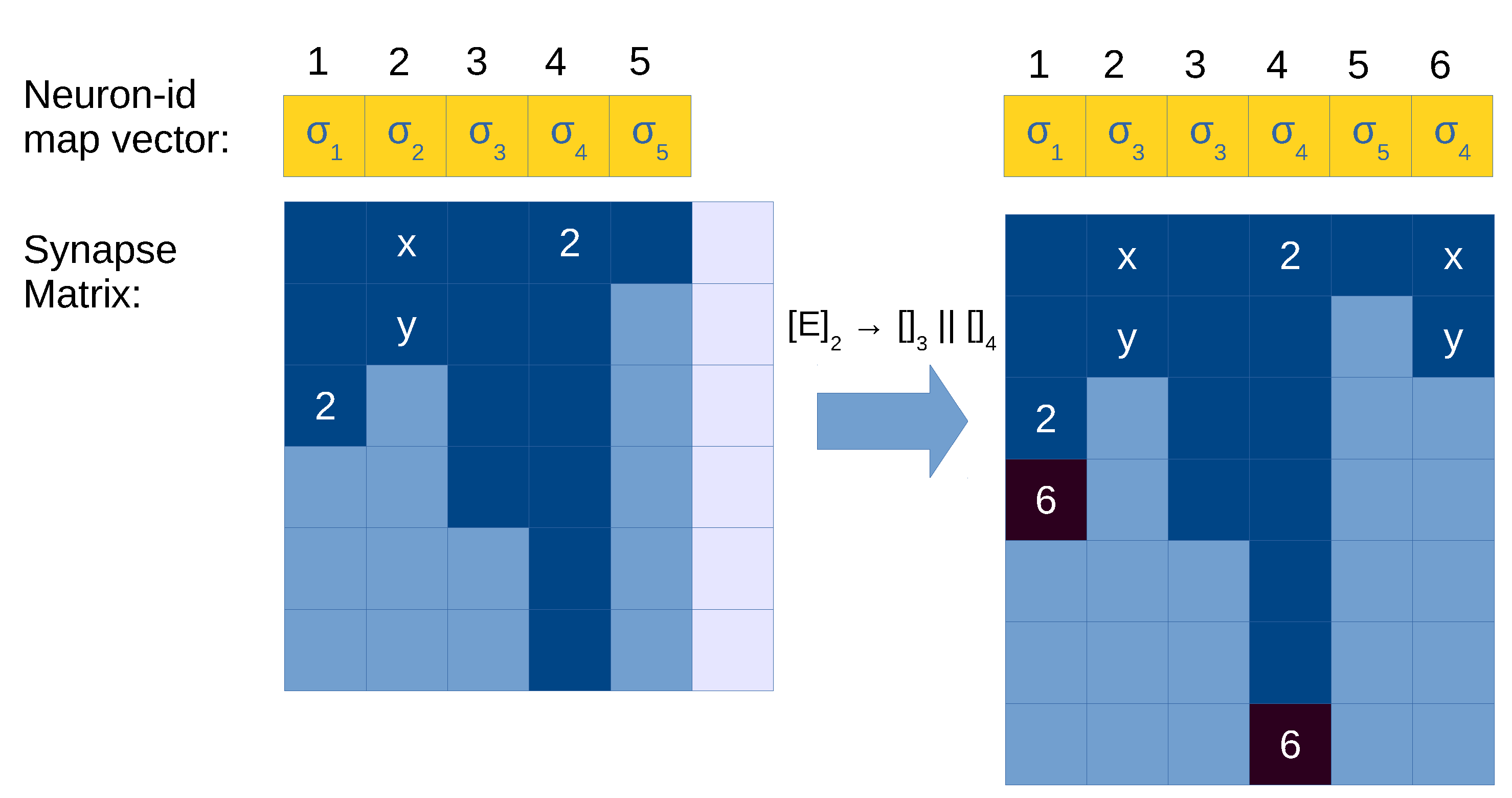
In order to achieve this separation, it is enough to have a vector to map each neuron id to its label. We will call this new vector, neuron-id map vector , and the following holds at step k: . That is, neuron-id map vector, configuration vector and spiking vector have a size of as well. Once the label of a neuron is obtained, the information of its corresponding rules can be accessed as usual, like the neuron-rule map vector . For simplicity, we attach the neuron-id map vector to the transition tuple. Moreover, the synapse matrix becomes dynamic, thus using k sub-index: ; hence, the transition matrix is also dynamic. Let us now introduce this new notation for transition tuple and transition matrix:
The transition matrix is now a dynamic pair: .
The transition tuple is extended as follows: .
We use the following encoding for each type of rule. Spiking and forgetting rules remain unchanged:
For a budding rule as . Given that all pairs in the rule vector are of the form , and c is always greater equal than 1, then we can encode a budding rule as a pair .
For a division rule as . Given that all pairs in the rule vector are of the form , and c is always greater equal than 1, then we can encode a division rule as a pair .
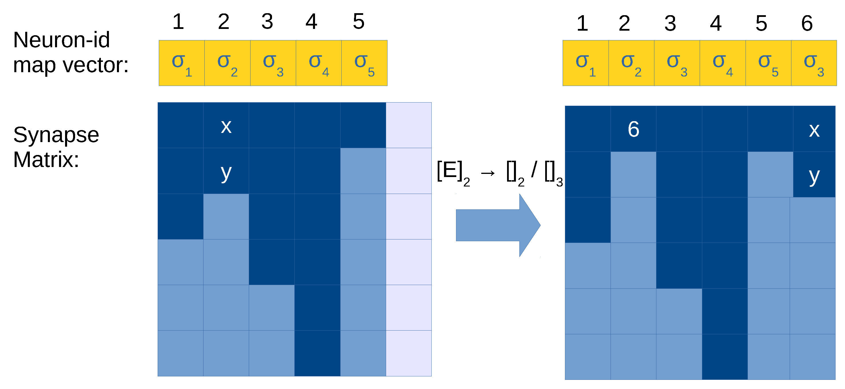
The execution of a budding rule
requires the following operations (see
Figure 5 for an illustration):
Let be the neuron id executing this rule.
Allocate a column to the synapse matrix for the new neuron, and use this index as its neuron id.
Add an entry to the neuron-id map vector at position with the label l.
Copy column to the new column in .
Delete the content of column and add only one element at the first row with the id .
Figure 5.
Illustration of application of a budding rule in the synapse matrix with compressed representation. Light blue cells in the synapse matrix are empty values (0), dark cells are positions with values greater than 0 (i.e., with neuron id), and light cells are empty columns allocated in memory (a total of ). Neuron 1 is applying budding, and its content is copied to an empty column (5) and replaced by a single synapse to the created neuron.
For a division rule
, the following operations have to be performed (see
Figure 6 for an example):
Let be the neuron id executing this rule.
Allocate a new column for the created neuron l in the synapse matrix .
Modify the neuron-id map vector as follows: replace the value at position for label j, and add a new entry for to associate it with label k.
Copy column to in (the generated neuron gets the out synapses of the parent).
Find all occurrences of in the synapse matrix, and add to the columns where it is found.
Figure 6.
Illustration of application of a division rule in the synapse matrix with compressed representation. Light blue cells in the synapse matrix are empty values (0), dark cells are positions with values greater than 0 (i.e., with neuron id), and light cells are empty columns allocated in memory (a total of ). Neuron 1 is being divided, and its content is copied to an empty column (5). Columns 0 and 3 represent neurons with a synapse to the neuron being divided (1), so we need to update them as well with the synapse to the created neuron (5). Neuron 3 has reached its limit of maximum out degree, therefore we need to expand the matrix with a new row, or use a COO-like system to store these exceeded elements.
The last operation can be very expensive if the amount of neurons is large, since it requires to loop all over the synapse matrix. Moreover, when adding
in all the columns containing
, it would be possible to exceed the predetermined size
z. For this situation, a special array of overflows is needed, like ELL + COO format for SpMV [
41]. For simplicity, we will assume this situation is weird and the algorithm will allocate a new row for the synapse matrix.
Some functions in the pseudocode are re-defined to support dynamic networks with division and budding:
INIT functions as in Algorithm 7. They now take into account the initialization of structures at its maximum amount , including the new neuron-id map vector.
SPIKING_VECTORS function, as defined in Algorithm 4 and modified in
Section 3.2 for optimized matrix representation, is slightly modified (just two lines) to support the neuron-id map vector.
APPLICABLE function as in Algorithm 8. This function, when dealing with division rules, has to search if there are existing synapses for the neurons involved. If they exist, the division rule does not apply.
COMPUTE_NEXT function as in Algorithm 9, to include the operations described above. It now needs to expand the synapse matrix either by columns (when new neurons are created) or by rows if there is a neuron from which we need to create a synapse to the new neuron and it has already the maximum out degree z. In this case, we need to re-allocate the synapse matrix in order to extend it by one row (this is written in the pseudocode with the function EXPAND_MATRIX). Finally, let us remark that we can easily detect if type of a rule at it’s associated value: if 0, it is a budding rule, if it is positive number, a spiking rule, otherwise (negative value) it is a division rule.
| Algorithm 7 Initialization functions for dynamic SNP systems with budding and division rules over optimized compressed matrix representation. |
- 1:
procedureINIT() - 2:
INIT_NEURON_VECTORS() - 3:
INIT_RULE_MATRICES() - 4:
- 5:
return - 6:
end procedure - 7:
procedureINIT_NEURON_VECTORS() - 8:
- 9:
EMPTY_VECTOR() - 10:
EMPTY_VECTOR() - 11:
- 12:
for all do - 13:
- 14:
- 15:
- 16:
end for - 17:
return - 18:
end procedure - 19:
procedureINIT_RULE_MATRICES() - 20:
- 21:
EMPTY_VECTOR(m) - 22:
EMPTY_VECTOR(m) - 23:
for all do - 24:
- 25:
- 26:
- 27:
end for - 28:
EMPTY_VECTOR() - 29:
EMPTY_MATRIX() - 30:
for do - 31:
- 32:
- 33:
for all do - 34:
- 35:
- 36:
end for - 37:
end for - 38:
- 39:
return - 40:
end procedure
| ▹ Initialize vectors only related to neurons. ▹ Initialize matrices related to rules. ▹ Get information from ▹ Create initial configuration ▹ Create neuron-rule vector ▹ For each neuron ▹ Get info of the neuron from ▹ Initial configuration ▹ Neuron-rule map vector initialization ▹ Get information from ▹ Create preconditions vector ▹ For each rule (column). This loop is parallelizable. ▹ Get info of the rule ▹ Store it in precondition vector ▹ Store it in rule vector ▹ For each neuron label ▹k is our iterator, compacting the rows ▹ For each out synapse ▹ We know that
|
| Algorithm 8 Applicable functions for dynamic SNP systems with budding rules over optimized compressed matrix representation. |
- 1:
procedureAPPLICABLE() - 2:
- 3:
- 4:
- 5:
- 6:
if then - 7:
return - 8:
- 9:
- 10:
while do - 11:
- 12:
- 13:
end while - 14:
return - 15:
else - 16:
- 17:
- 18:
while do - 19:
- 20:
- 21:
end while - 22:
for do - 23:
▹ Either or - 24:
- 25:
while do - 26:
- 27:
- 28:
end while - 29:
end for - 30:
return - 31:
end if - 32:
end procedure
| ▹ Get some content of transition tuple ▹ Get some content of transition matrix ▹ Preconditions of the rule ▹ Preconditions of the rule ▹ If a spiking or forgetting rule ▹ If rule j is applicable in neuron i▹ If a budding rule ▹ Check if synapse exists ▹ Until an empty value or the maximum ▹ If synapse exists ▹ If a division rule ▹ Check if synapse or exists ▹ Until an empty value ▹ If either synapse exists ▹ Search for neurons with label or ▹ Either or ▹ Combination of conditions ▹ If the synapse exists
|
| Algorithm 9 Compute next function for dynamic SNP systems with budding and division rules using optimized compressed matrix representation. |
- 1:
procedureCOMPUTE_NEXT() - 2:
- 3:
- 4:
- 5:
- 6:
for do - 7:
- 8:
if then - 9:
- 10:
if then - 11:
- 12:
- 13:
while do - 14:
- 15:
- 16:
- 17:
end while - 18:
else if then - 19:
- 20:
- 21:
- 22:
for do - 23:
- 24:
if then - 25:
- 26:
else - 27:
- 28:
end if - 29:
end for - 30:
else - 31:
- 32:
- 33:
- 34:
- 35:
- 36:
for do - 37:
- 38:
end for - 39:
for do - 40:
- 41:
- 42:
while do - 43:
- 44:
- 45:
end while - 46:
if b then - 47:
if then - 48:
- 49:
EXPAND_MATRIX() - 50:
end if - 51:
- 52:
end if - 53:
end for - 54:
end if - 55:
end if - 56:
end for - 57:
return - 58:
end procedure
| ▹ Create a copy of ▹ Extract info from transition tuple ▹ Extract info from transition matrix ▹ Get current amount of neurons. ▹ For each neuron. This loop is parallelizable. ▹ Index of rule to fire in the neuron ▹ Only if there is a rule. ▹ Get rule info ▹ Execution of a spiking or forgetting rule ▹ Consume spikes in firing neuron ▹ Next while stops if , i.e., a firing rule ▹ Until an empty value ▹ Get connected neuron by a synapse ▹ Produce spikes in connected neuron ▹ Execution of a budding rule ▹ Increment counter of neurons ▹ Empty the neuron i, neuron is 0 already ▹ is the label of the new neuron ▹ Copy column i to the new one ▹ Update out synapses of i ▹ The only new out synapse of i ▹ No more out synapses for i ▹ Execution of a division rule ▹ Get new neurons labels ▹ Increment counter of neurons ▹ Empty the neuron i, neuron is 0 already ▹ The new label of the neuron ▹ The label of the new neuron ▹ Copy out synapses to new neuron ▹ Copy column i to the new one ▹ Search for in synapses of neuron i ▹ Boolean saying the synapse was found ▹ Search the end of the column ▹ Search for neuron i ▹ If synapse was found, add new neuron at the end of the column ▹ The neuron x has a larger out degree than z ▹ Extend with one more row ▹ This can lead to overflows if
|
3.3.2. Plasticity Rules
For dynamic SNP systems with plasticity rules, the synapse matrix can be allocated in advance to the exact size q, since no new neurons are created. Thus, there is no need of using a neuron-id map vector as before. However, enough rows (value z) in the synapse matrix have to be pre-established to support the maximum amount of synapses. Fortunately, this can be pre-computed by looking to the initial out degrees of the neurons and the size of the neuron sets in the plasticity rules adding synapses. We encode a plasticity rule , with as follows: . Next, we define the value of for SNP systems with plasticity rules: , where . In other words, is the maximum out degree (z) that a neuron can have initially plus those new connections that can be created with plasticity rules inside that neuron. This result can be refined for plasticity rules having , because we know up to k new synapses can be created at a time. However, for simplicity, we will use the formula above.
First, we need to represent plasticity rules into vectors. We assume that is the total amount of plasticity rules in the system, and that there is a total order between these rules. Given a plasticity rule, we can initialize the neuron-map and the precondition vector as with spiking rules. But in this case, we need a couple of new vectors and modify existing ones in order to represent all plasticity rules , with (following the imposed total order):
Rule vector stores the following pair for a plasticity rule : , that is, the consumed spikes and the unique index of the plasticity rule j. This index is used to access the following vector, and it is stored as a negative value in order to detect that this is a plasticity rule.
Plasticity rule vector, of size , contains a tuple for each plasticity rule of the form . The values and are used as indexes, from (start) to (end) for the following vector.
Plasticity neuron vector, of size , represents all neuron sets of plasticity rules. Thus, the elements of are stored, in an ordered way, between to .
Time vector is used to prevent neurons from applying rules during one step if the plasticity rule applied was of the type . It contains binary (0 or 1) values.
Transition matrix is therefore . Note that the Synapse matrix can be modified at each step, so we use sub-index k.
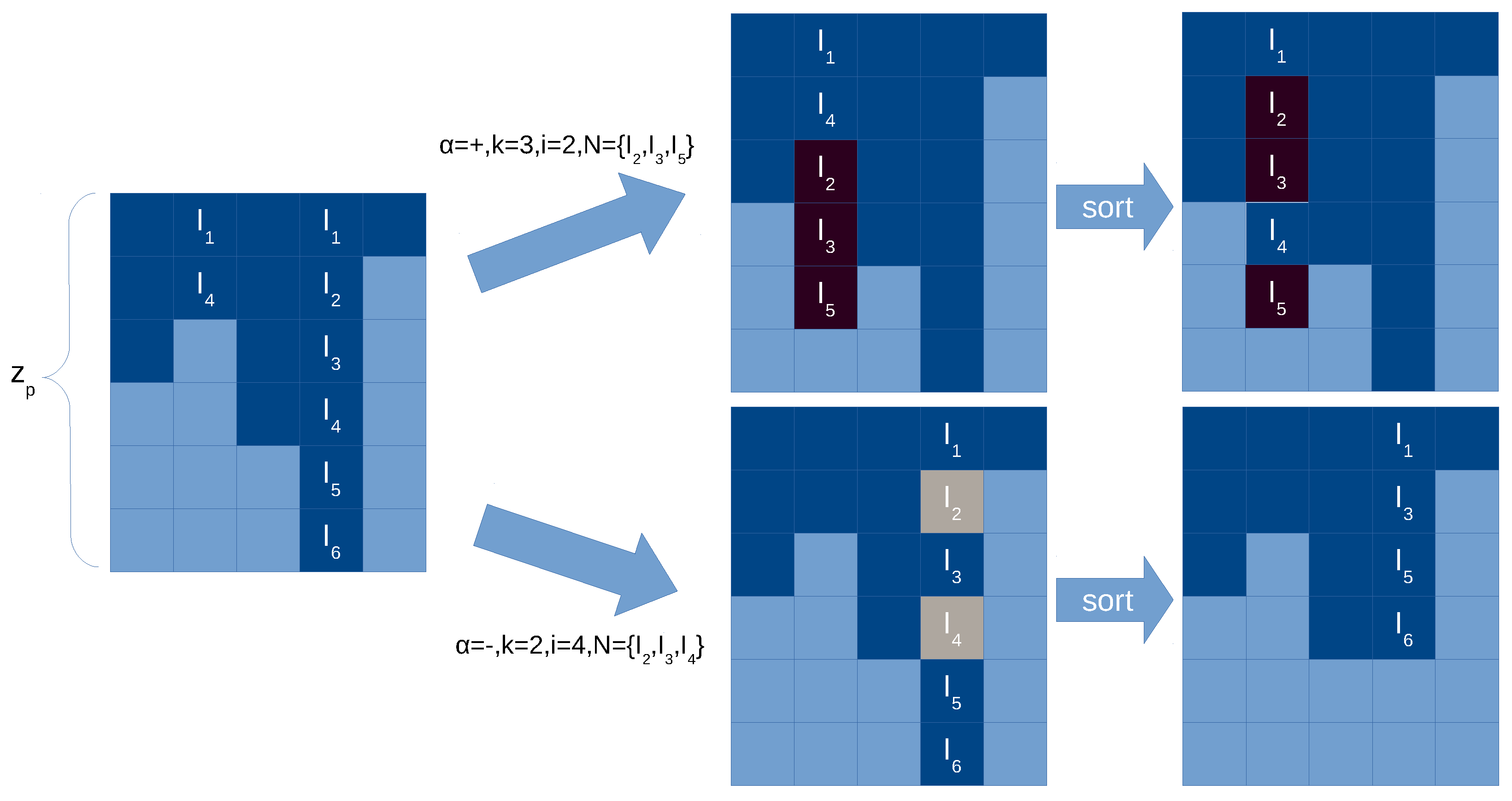
The following operations have to be performed to reproduce the behavior plasticity rules (see
Figure 7 for an illustration):
Figure 7.
Illustration of application of a plasticity rule in the synapse matrix with compressed representation. Light blue cells in the synapse matrix are empty values (0), dark cells are positions with values greater than 0 (i.e., with neuron label). Two examples are give, in case of adding new synapses (top) and in case of deleting synapses (bottom). We sort the synapses per column for more efficiency.
Checking the applicability of plasticity rules is much simpler than for division rules, given that the preconditions only affect to the local neuron and we do not need to know if there are existing synapses. However, for a plasticity rule r in a neuron i, and in order to create new or delete existing synapses, we need to check which neurons declared in r are already in the column i in the synapse matrix. This search can be , being the length of the neuron set in r. Nevertheless, by maintaining always the order in the column, this search can be done easily in .
Given that it is not usual to have budding and division rules together with plasticity rules, the pseudocode is based on the optimized matrix representation for static SNP systems (and not for division and budding) in
Section 3.2. Algorithm 10 shows the re-definition of INIT_RULE_MATRICES and COMPUTE_NEXT functions, replacing those from Algorithm 3. For COMPUTE_NEXT, the implementation is very similar to the original one, but it just call to a new function, PLASTICITY, which actually modify the synapses of the neuron (by just modifying its corresponding column in the synapse matrix). This function and its auxiliaries are defined in Algorithms 11 and 12, respectively.
| Algorithm 10 Functions for dynamic SNP systems with plasticity rules using optimized compressed matrix representation. |
- 1:
procedureINIT_RULE_MATRICES() - 2:
- 3:
EMPTY_VECTOR(m) - 4:
EMPTY_VECTOR(m) - 5:
EMPTY_VECTOR() - 6:
EMPTY_VECTOR() - 7:
- 8:
- 9:
for all do - 10:
if then - 11:
- 12:
- 13:
else if then - 14:
- 15:
- 16:
- 17:
SORT() - 18:
- 19:
- 20:
end if - 21:
end for - 22:
EMPTY_VECTOR(q) - 23:
EMPTY_MATRIX() - 24:
for all do - 25:
- 26:
for all do - 27:
- 28:
- 29:
end for - 30:
end for - 31:
- 32:
return - 33:
end procedure -
- 34:
procedureCOMPUTE_NEXT() - 35:
- 36:
- 37:
- 38:
for do - 39:
- 40:
if then - 41:
- 42:
- 43:
if then - 44:
- 45:
while do - 46:
- 47:
- 48:
- 49:
end while - 50:
else if then - 51:
PLASTICITY() - 52:
- 53:
end if - 54:
end if - 55:
- 56:
end for - 57:
- 58:
return - 59:
end procedure
| ▹ Get information from , is different for plasticity. ▹ Create preconditions vector ▹ Create rule vector ▹ Create plasticity rule vector ▹ Create plasticity neuron vector ▹ Counter for plasticity rule vector ▹ Counter for plasticity neuron vector ▹ For each rule (column). This loop is parallelizable. ▹ If spiking rule ▹ Store it in precondition vector ▹ Store it in rule vector ▹ If plasticity rule ▹ Store it in precondition vector ▹ Store it in rule vector ▹ Store it in rule vector ▹ Sort and store in after position ▹ Create time vector ▹ Create synapse matrix ▹ For each neuron (column in synapse matrix) ▹k is our iterator, compacting the rows ▹ For each out synapse ▹ We know that ▹ New transition matrix ▹ Create a copy of ▹ Get some content of transition tuple ▹ For each neuron. This loop is parallelizable. ▹ Index of rule to fire in the neuron ▹ Only if there is a rule or blocked neuron ▹ Get rule info ▹ Consume spikes in firing neuron ▹ If a spiking rule ▹ Until an empty value or the maximum ▹ Get connected neuron by a synapse ▹ Produce spikes in connected neuron ▹ If a plasticity rule ▹ Modify only column i ▹ Reset time vector ▹ Next transition matrix
|
4. Algorithms
In this section we define the algorithms implementing the methods described in
Section 3.
Let us first define a generic function to create a new, empty (all values to 0) vector of size s as follows: EMPTY_VECTOR(s). In order to create an empty matrix with f rows and c columns, we will use the following function: EMPTY_MATRIX(). Next, the pseudocodes for simulating static SNP systems with sparse representation are given. Algorithm 3 shows the INIT and COMPUTE_NEXT functions, while Algorithm 4 shows the selection of spiking vectors.
For ELL-based matrix representation for static SNP systems, we need to re-define only two functions (INIT_RULE_MATRICES and COMPUTE_NEXT) from Algorithm 3 (static SNP systems with sparse representation) as shown in Algorithm 5.
For our optimized matrix representation for static SNP systems, we need to re-define only two functions (INIT_RULE_MATRICES and COMPUTE_NEXT) from Algorithm 3 (static SNP systems with sparse representation) as shown in Algorithm 6. Moreover, the following two lines in the definition of COMBINATIONS function at Algorithm 4 are required, in order to support a spiking vector of size q:
For
dynamic SNP systems with budding and division rules, the following functions are redefined: INIT functions as in Algorithm 7, APPLICABLE function as in Algorithm 8, and COMPUTE_NEXT function as in Algorithm 9. The SPIKING_VECTORS function, as defined in Algorithm 4 and modified in
Section 3.2 for optimized matrix representation, is slightly modified (just two lines) to support the neuron-id map vector as follows:
Line 6 at Algorithm 4:
Line 18 at Algorithm 4: for
For
dynamic SNP systems with plasticity rules, the pseudocode is based on the optimized matrix representation for static SNP systems (and not for division and budding) in
Section 3.2. Algorithm 10 shows the re-definition of INIT_RULE_MATRICES and COMPUTE_NEXT functions, replacing those from Algorithm 3. As for line 17, we assume that the function SORT exists, which takes a set of neurons, sorts them by id, and generates a vector. Moreover, we can copy vectors directly from one position by just one assignation. The new PLASTICITY function is defined in Algorithm 11, and its auxiliaries are defined in Algorithm 12.
| Algorithm 11 Function for plasticity mechanism using optimized compressed matrix representation. |
- 1:
procedurePLASTICITY() - 2:
- 3:
- 4:
EMPTY_VECTOR() - 5:
for do - 6:
- 7:
end for - 8:
- 9:
if then - 10:
DEL_SYNAPSES() - 11:
else if then - 12:
ADD_SYNAPSES() - 13:
else if then - 14:
ADD_SYNAPSES() - 15:
DEL_SYNAPSES() - 16:
- 17:
else if then - 18:
DEL_SYNAPSES() - 19:
ADD_SYNAPSES() - 20:
- 21:
end if - 22:
return () - 23:
end procedure
| ▹ Get info of plasticity rule ▹ Number of neurons in the neuron set ▹ Create a vector with the neuron set ▹ Copy the contents of the neuron set ▹ Vale for time vector, only 1 for ▹ Delete synapses ▹ Add synapses ▹ Add and delete synapses ▹ Delete and add synapses
|
| Algorithm 12 Auxiliary functions for plasticity mechanism using optimized compressed matrix representation. |
- 1:
procedureDEL_SYNAPSES() - 2:
INTERSEC() - 3:
if then - 4:
DELETE_RANDOM() - 5:
end if - 6:
- 7:
- 8:
while do - 9:
if then - 10:
- 11:
- 12:
else - 13:
if then - 14:
- 15:
- 16:
end if - 17:
- 18:
end if - 19:
- 20:
end while - 21:
return A - 22:
end procedure - 23:
procedureADD_SYNAPSES() - 24:
DIFF() - 25:
if then - 26:
DELETE_RANDOM() - 27:
end if - 28:
- 29:
EMPTY_VECTOR() - 30:
- 31:
while do - 32:
if then - 33:
- 34:
- 35:
else - 36:
- 37:
- 38:
end if - 39:
- 40:
end while - 41:
return B - 42:
end procedure
| ▹ Calculate (involved synapses to be deleted) ▹ If more than k neurons, select randomly ▹ A random set of k neurons ▹ The new amount of synapses to delete ▹ Initialize iterators ▹ Loop over the column ▹ Synapse to delete ▹ Delete the synapse ▹ Advance in vector ▹ Need to compact the vector ▹p is the last compacted position ▹ Advance the last compacted position p ▹ Calculate (not involved synapses to create) ▹ If more than k neurons, select randomly ▹ A random set of k neurons ▹ The new amount of synapses to delete ▹ Create the output ▹ Initialize iterators ▹ Loop over the column ▹ Synapse to add ▹ Add the synapse ▹ Keep the synapse
|
In order to keep Algorithm 12 simple, we assume that the functions INTERSEC, DIFF, and DELETE_RANDOM are already defined. As mentioned above, INTERSEC and DIFF can be implemented with algorithms of complexity , given that the vectors (a column of synapse matrix and a chunk of plasticity neuron vector) are already sorted. We also assume that DELETE_RANDOM is a function that randomly select k elements from a total of n while keeping the order between elements. This can be done with an algorithm of complexity .
5. Results
In this section we conduct a complexity analysis (for both time and memory) of the algorithms. In order to define the formulas, we need to introduce a set of descriptors for a spiking neural P system
. These are described in
Table 1. Moreover,
Table 2 summarizes the vectors and matrices employed by each representation, and their corresponding sizes defined according to the descriptors. We use the following short names for the representations: Sparse (original sparse representation as
Section 3), ELL (ELL compressed representation as in
Section 3.1), optimized static (optimized static compressed representation as in
Section 3.2), division and budding (optimized dynamic compressed representation for division and budding as in
Section 3.3.1), and plasticity (optimized dynamic compressed representation for plasticity as in
Section 3.3.2).
According to
Table 2, we can limit the value of
for dynamic SNP systems with division and budding with the following formula:
, where
is the maximum amount of memory in the system (measured in the word size employed to encode the elements of all the matrices and vectors; e.g., 4 Bytes). Moreover, we can infer when the matrix representation will be smaller for static SNP systems: ELL is better than sparse when
; optimized is better than ELL when
; optimized is better than sparse when
. In other words, our optimized compressed representation is worth when the the maximum out degree of the neurons is less than the total number of rules minus 2.
For dynamic SNP systems, given can say that a solution to a problem using an SNP with plasticity rules is better than a solution based on division and budding, if ; in other words, if we can know the maximum amount of neurons to generate, and this number is greater than a formula based on number of initial neurons, number of rules, and number of elements in the neuron set and the max out degree, then the solution will need less memory using plasticity.
Finally,
Table 3 shows the order of complexity of each function as defined for each representation. We can see that COMPUTE_NEXT gets reduced in complexity as well when using optimized static representation against ELL and sparse, given that we expect that
, and also
. However, we can see that implementing division and budding explodes the complexity of the algorithms, since they need to loop over all the neurons checking for in-synapses. This also depends on the total amount of generated neurons in a given step. This is also the case for the generation of spiking vectors, because the applicability function also needs to loop over all existing neurons. However, for dynamic networks, plasticity keeps the complexity with the amount of neurons, the value
z, and the descriptors of plasticity rules (max value of
k and amount of neurons in a neuron set
).
Therefore, we can see that using our compressed representations, both the memory footprint of the simulators and their complexity are reduced, as long as the maximum out degree of neurons is a low number. Furthermore, we can see that for dynamic networks, plasticity is an option that keeps the complexity balanced, since we know in advance the amount of neurons and synapses.
Let us make an easy example of comparison with an example from the literature. For example, if we take the SNP system for sorting natural numbers as defined in [
42], then we have that
,
and
, where
n is the amount of natural numbers to sort. Thus:
The size of the sparse representation is and the complexity of COMPUTE_NEXT is .
The size of the ELL representation is and the complexity of COMPUTE_NEXT is .
The size of the optimized representation is and the complexity of COMPUTE_NEXT is .
The optimized representation drastically decreases the order of complexity and amount of memory spent for the algorithms, going from orders of
to
. ELL has a similar order of complexity to that of sparse, but the amount of memory is just a bit decreased.
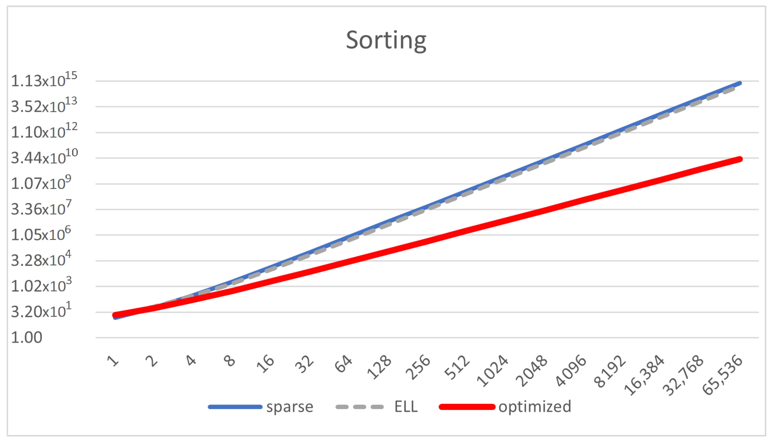
Figure 8 shows that the reduction of the memory footprint achieved with the compressed representations takes effect after
.
Figure 9 shows that the optimized representation scales better than ELL and sparse. ELL is only a bit better than the sparse representation, demonstrating the need for using the optimized one, which significantly scales much better.
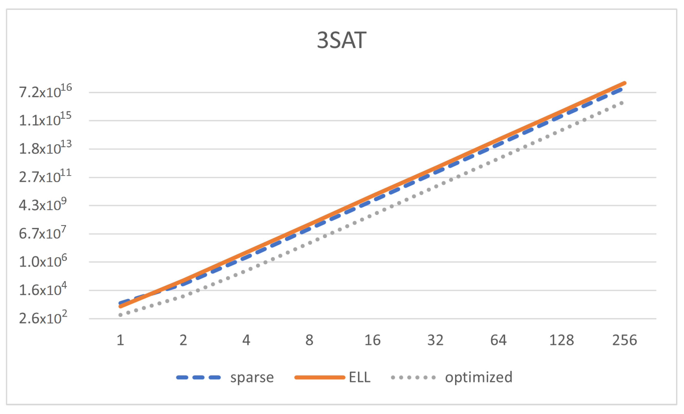
Finally, we also analyze a uniform solution to 3SAT with SNP systems without delays as in [
43] (
Figure 10). We can see that
,
and
, where
n is the amount of variables in the 3SAT instance. We can see that
, so our optimized implementation will be able to save some memory. Therefore:
The size of the sparse representation is and the complexity of COMPUTE_NEXT is .
The size of the ELL representation is and the complexity of COMPUTE_NEXT is .
The size of the optimized representation is and the complexity of COMPUTE_NEXT is .
Figure 10.
Memory size of the matrix representation (Y-axis in log scale) depending on the number of variables in the SAT formula (, X-axis in log scale) for the model of 3SAT, using sparse, ELL, and optimized representation.
Figure 10.
Memory size of the matrix representation (Y-axis in log scale) depending on the number of variables in the SAT formula (, X-axis in log scale) for the model of 3SAT, using sparse, ELL, and optimized representation.
We can see that the memory footprint is decreased but it is still of the same order of magnitude (
), and the same happens with the computing complexity. Thus, our representation helps to reduce memory, although not significantly for this specific solution. This is mainly due to having a high value of
z. We can see in
Figure 10 how the reduction of memory takes place only for optimized representation as long as
n increases. It is interesting to see that the ELL representation is even worse than just using sparse representation.
Finally, let us analyze the size of the solution uniform solution to subset sum with plasticity rules in [
34]. The descriptors for the matrix representation of a dynamic SNP system with plasticity rules are the following:
,
,
,
, where
n is the number of sets
V, therefore, the memory footprint is described as:
. If we were using a sparse representation where the transition matrix is of order
, then the amount of memory is of order
.
6. Conclusions
In this paper, we addressed the problem of having very sparse matrices in the matrix representation of SNP systems. Usually, the graph defined for an SNP system is not fully connected, leading to sparse matrices. This drastically downgrades the performance of the simulators. However, sparse matrices are a known issue in other disciplines, and efficient representations have been introduced in the literature. There are even solutions tailored for parallel architectures such as GPUs.
We propose two efficient compressed representations for SNP systems, one based on the classic format ELL, and an optimized one based on a combination of CSR and ELL. This representation gives room to support rules for dynamic networks: division, budding, and plasticity. The representation for plasticity poses more advantages than the one for division and budding, since the synapse matrix size can be pre-computed. Thus, no label mapping nor empty columns to host new neurons are required. Moreover, simulating the creation of new neurons in parallel can damage the performance of the simulator significantly, because this operation can be sequential. Plasticity rules do not create new neurons, so this is avoided.
As future work, we plan to provide implementations of these designs within cuSNP [
21] and P-Lingua [
44] frameworks to provide high performance simulations with real examples from the literature. We believe that these concepts will help to bring efficient tools to simulate SNP systems on GPUs, enabling the simulation of large networks in parallel. Specifically, we will use these designs to develop a new framework for automatically designing SNP systems using genetic algorithms [
45]. Another tool that could benefit from the inclusion of this new type of representation are visual tools for SNP systems [
46]. Moreover, our optimized designs will enable the effective usage of spiking neural P systems on industrial processes such as [
47,
48,
49,
50], and to optimization applications as [
51,
52]. SNP systems have been used in many applications [
5], and in order to be used in industrial applications we need efficient simulators where compressed representations of sparse matrices can help.
Numerical SNP systems (or NSNP systems) [
17,
53] are SNP system variants which are largely dissimilar to many variants of SNP systems, especially to the variants considered in this paper, for at least two main reasons: (1) rules in NSNP systems do not use regular expressions, and instead use linear functions, so that rules are applied when certain values or threshold of the variables in such functions are satisfied, and (2) the variables in the functions are real-valued, unlike the natural numbers associated with strings and regular expressions. One of the main goals in [
17] for introducing NSNP systems is to create an SNP system variant, which in a future work may be more feasible for use with training algorithms in traditional neural networks [
53]. For these reasons, we plan to extend our algorithms and compressed data structures for NSNP systems. We think that simulators for this variant can be effectively accelerated on GPUs. Specifically, GPUs are devices designed for floating point operations and not for integer arithmetic, although the latter is supported.
We also plan to include more models and ingredients into these new methods, such as delays, weights, dendrites, rules on synapses, and scheduled synapses, among others. Moreover, a recent work in SNP systems with plasticity shows that having the same set of rules in all neurons leads to Turing complete algorithms [
54]. This means that
m descriptor can be common to all neurons, leading to smaller representations for this kind of systems. We plan to study this deeper and combine it with our representations. Our aim on focusing on plasticity is also related to other results involving this ingredient in other fields such as machine learning [
55].


 ,
, 


