
Performance Evaluation of Epileptic Seizure Prediction Using Time, Frequency, and Time–Frequency Domain Measures


Abstract
1. Introduction
- 1
- We verify the importance of feature-specific in seizure prediction.
- 2
- We comprehensively summarize the features of time, frequency, and time–frequency domains and their interpretations in predicting seizures using EEG signals.
- 3
- The optimal features can provide guidance for studying each patient separately, and the several features summarized in these have implications for the general design principle of an epileptic prediction system.
2. Materials and Methodology
2.1. EEG Data
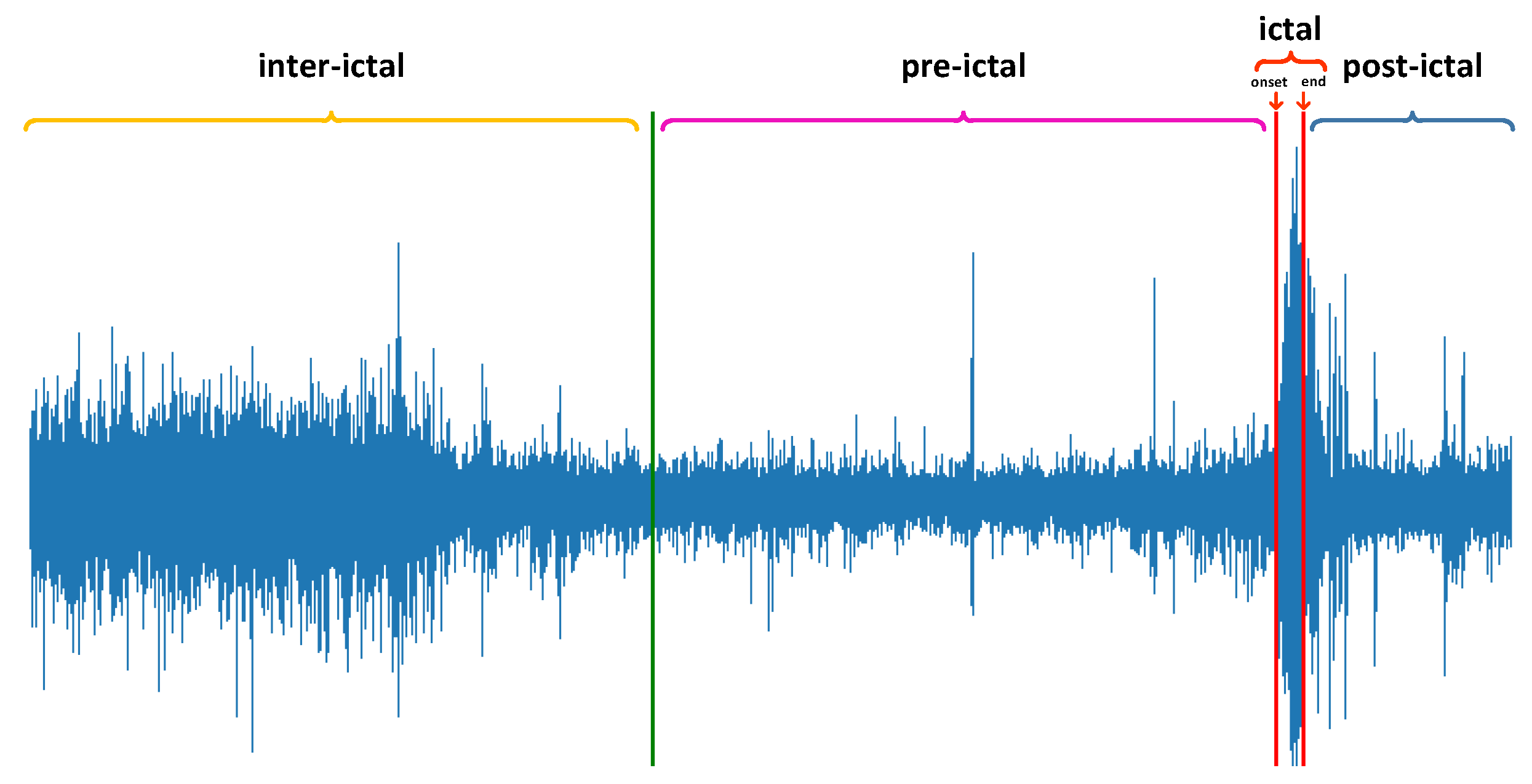
2.2. Preprocessing
- 1
- When the second seizure occurs within 15 min after the end of the first seizure, the data of the last seizure are discarded.
- 2
- Use the previous consecutive recording to supplement the data that do not satisfy 15 min.
- 3
- Any previous recording with a gap larger than 5 s from this recording is marked as disconsecutive.
- 4
- In the end, a duration of less than 15 min will also be used as a pre-ictal state of this seizure.
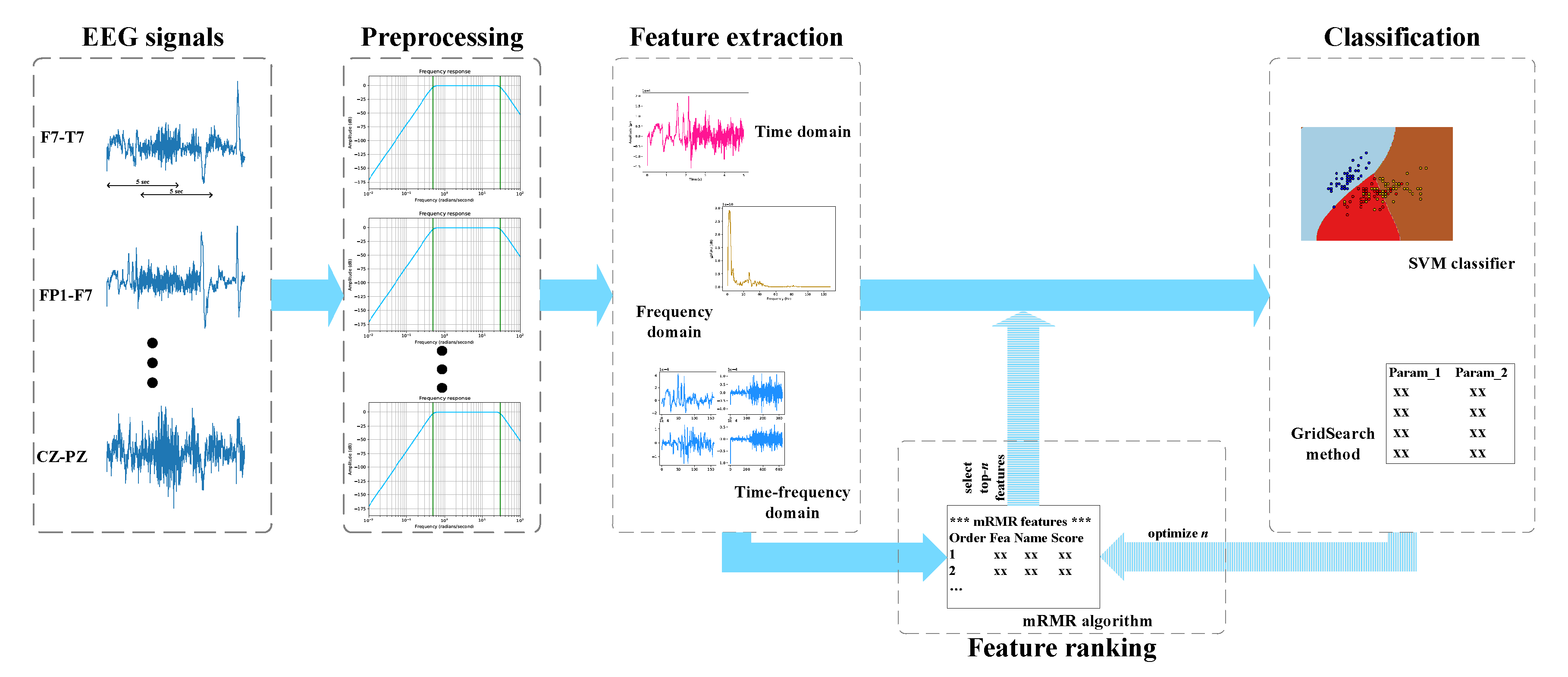
2.3. Feature Extraction
2.4. Feature Ranking
2.5. Classification
2.6. Performance Evaluation
| Algorithm 1: Finding optimal feature-channels using a sequential forward selection approach |
|
3. Results and Discussion
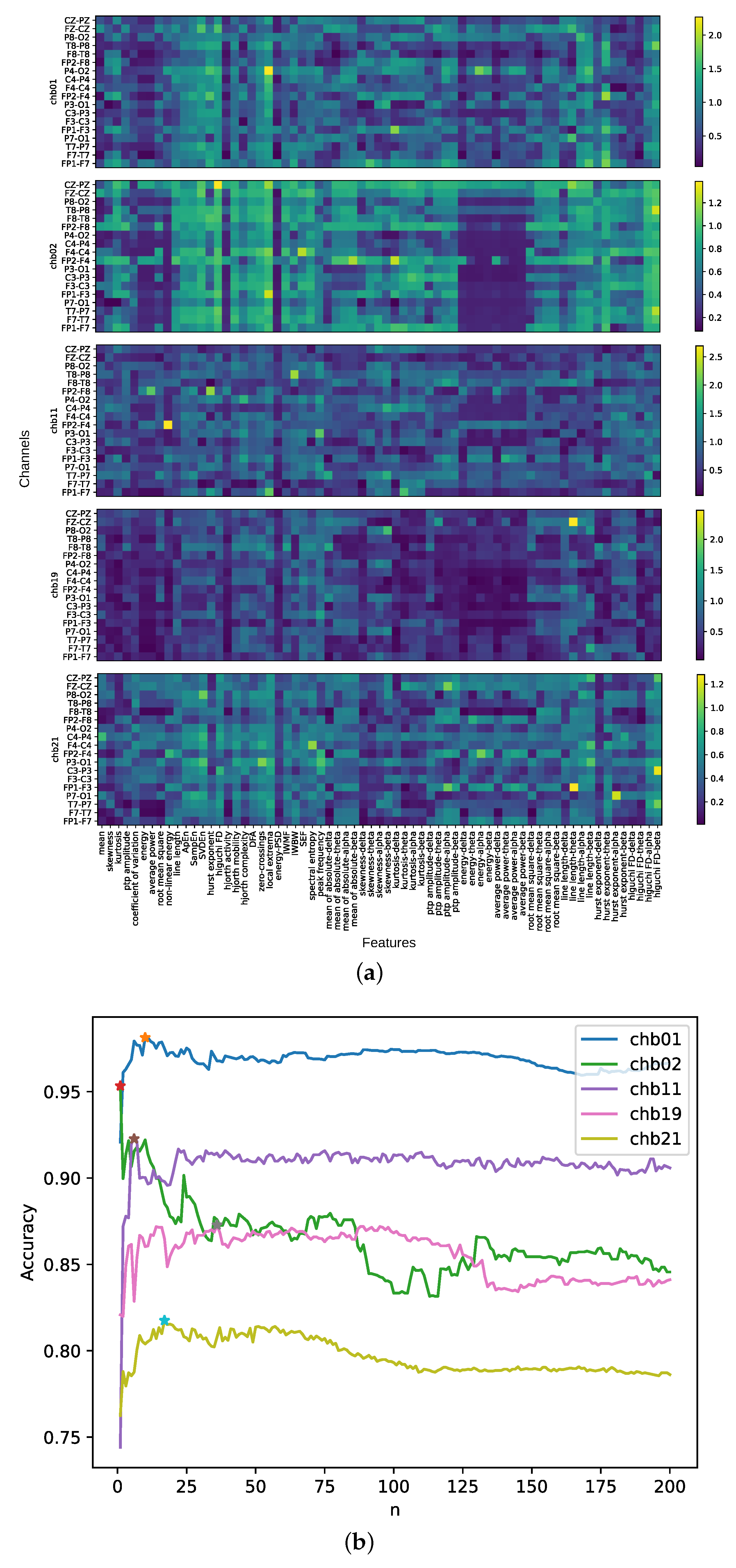
3.1. Performance of Different Numbers of Feature-Channels
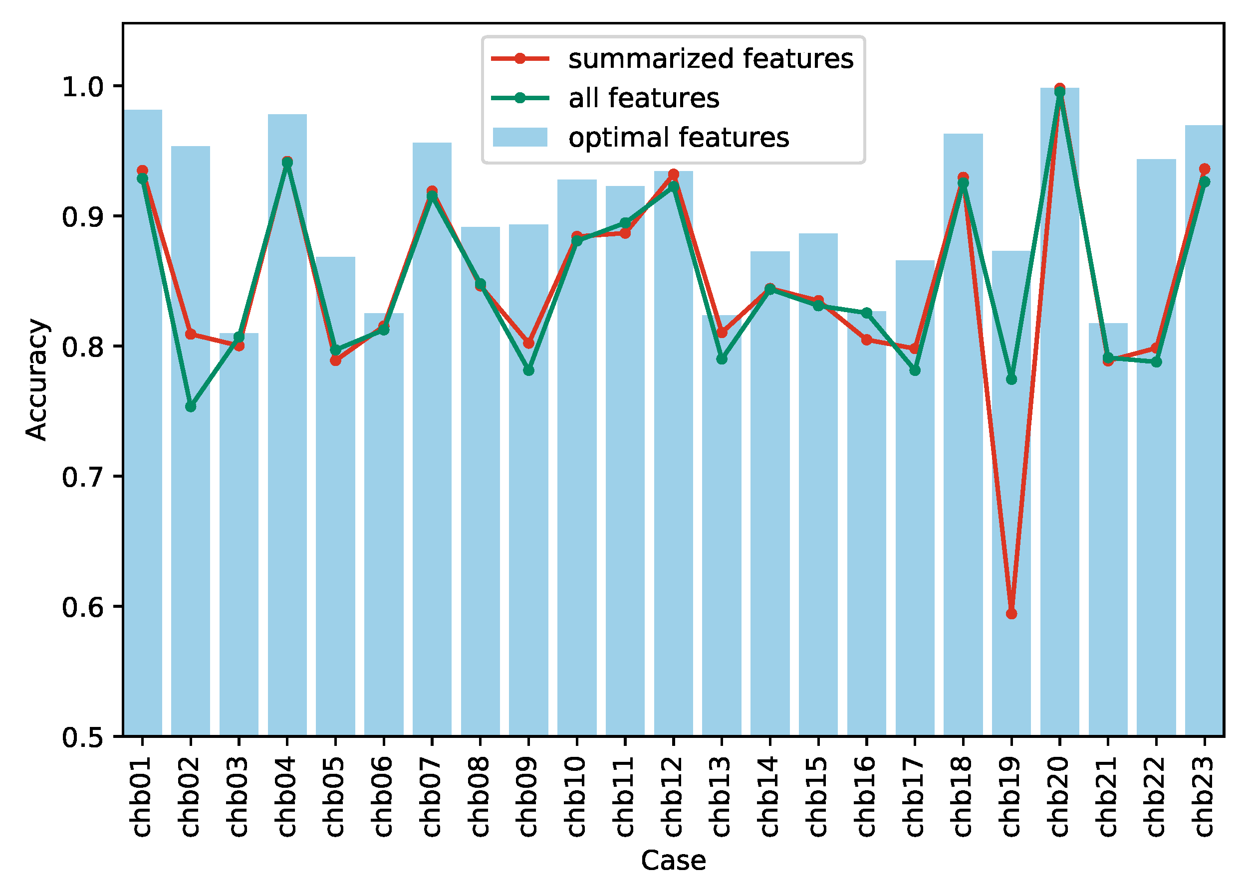
3.2. Comparison of Different Feature Design Principles
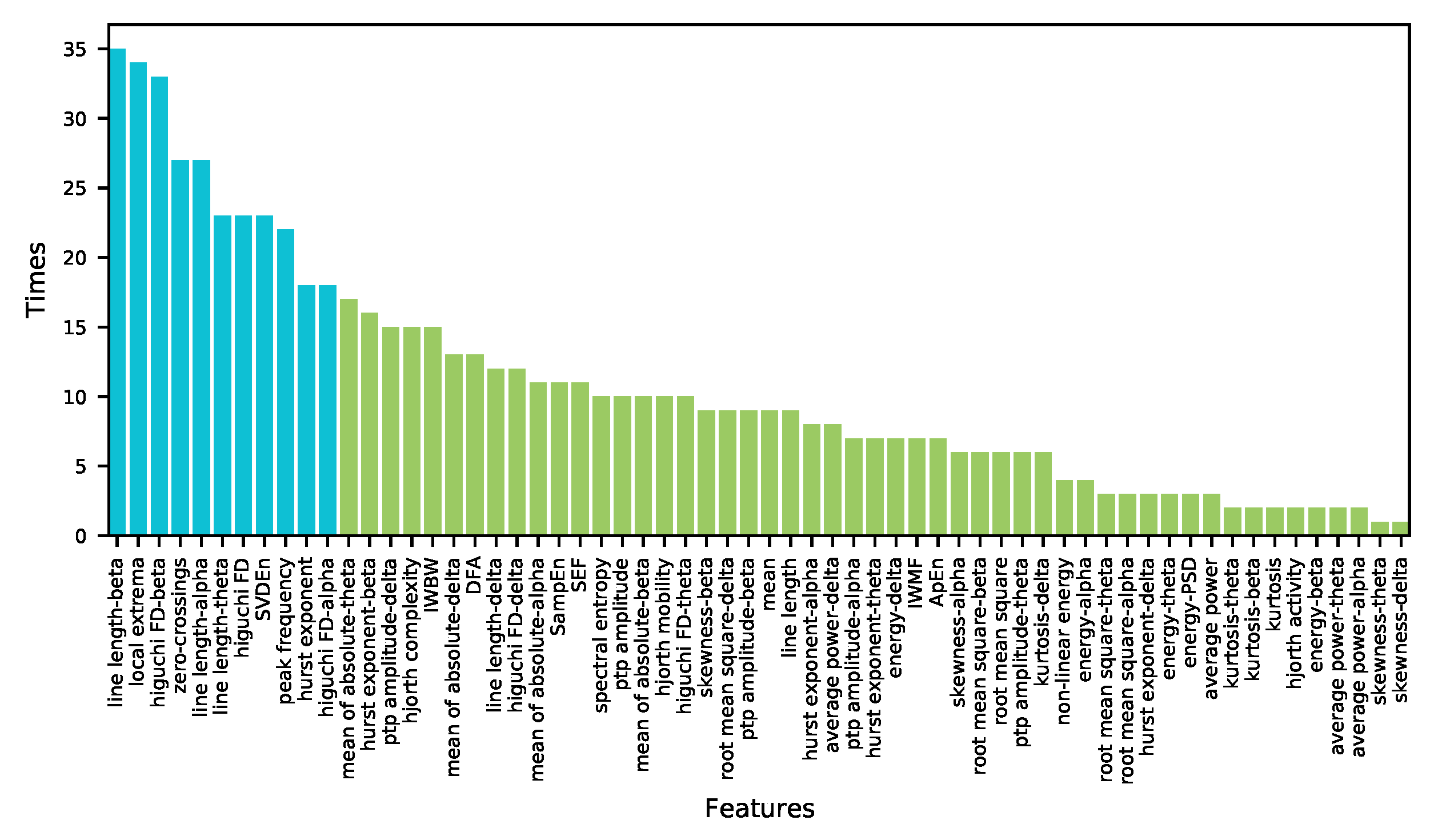
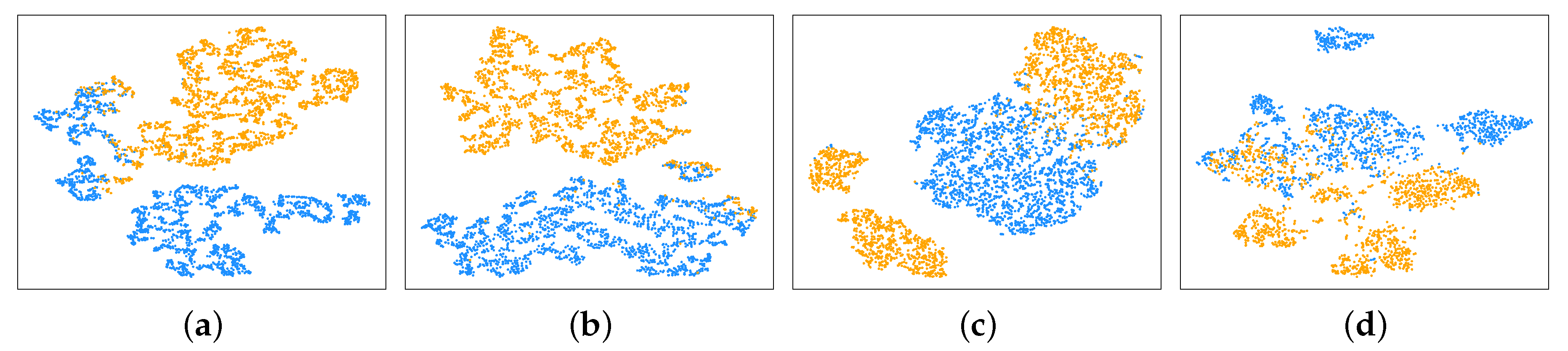
3.3. Visualization of Optimal Feature-Channels
3.4. Evaluation of Generalization Ability
3.5. Comparison to Prior Works
4. Conclusions
Author Contributions
Funding
Conflicts of Interest
Appendix A. Detailed Description of Features
Appendix A.1. Time Domain Features
- Basic statistics:Basic statistics features have been frequently used to distinguish pre-ictal pattern from an inter-ictal pattern. Mean, skewness, kurtosis, peak-to-peak amplitude, and coefficient of variation are used in this work. Skewness counting the asymmetry of the signal distribution is calculated as:where is the mean value, and is the standard deviation of signal X. Kurtosis can be used to measure the steepness of a signal as follows:Peak-to-peak amplitude quantifies the range of signal. Coefficient of variation is a normalized measures of signal dispersion, which is defined as the ratio of standard deviation to average value.
- Energy related:The energy is the sum of squares of the signal. The average power is the mean square of the signal, which is the average energy. The root mean square is the root mean square of the signal, which is the square root of the average power. The last energy related feature is nonlinear energy, which was originally presented in [25]. This feature can track the instantaneous frequency of the signal effectively, and its output is given by:
- Line length:Line length derived from Katz’s fractal dimension was first proposed by [26]. It increases as the amplitude or frequency of the signal increase. The normailzed line length can be represented as:
- Entropy based:Entropy, as the measure of uncertainty and disorder in the data, has been verified in a lot signal processing research. Approximate entropy (ApEn), sample entropy (SampEn), and singular value decomposition entropy (SVDEn) are the features used in this work. ApEn [27] can be used to quantify the regularity of the signal. The signal X is cut into subsequence for using m as the sliding window. Subsequence i is presented by . Then, the ApEn is defined as:where is the proportion of the distance between subsequence and all subsequence less than tolerance value . It can be calculated by:where is the Heaviside step function, and is the distance function. SampEn [28] is based upon concepts similar to ApEn. It is only for calculated other subsequences when calculation distance, so the corresponding to is:In addition, it performs logarithmic operations in the final entropy calculation. Therefore, the SampEn is defined by:Smaller values indicate more self-similar and regular signals, while larger values characterize higher complexity. SVDEn [29] measures the dimensionality of the signals. It uses the embedding matrix Y, which can be written as:where m is the embedding dimension, and j is the time delay. Then, this entropy is described as follows:where M is the number of the singular values of the embedding matrix Y and is the normalized singular value. Since SVDEn is calculated on all channels, the value can indicate a pattern of pre-ictal signal in both space and time.
- Hurst exponent:Hurst exponent can evaluate the predictability of a time series, and it has been proven that the epileptic brain is long term anticorrelated [30]. Rescaled range analysis is a commonly used calculation method in time series. The cumulative deviate series can be defined as follows:then compute the range:In addition, the standard deviation is:A Hurst exponent complies with the following rules:
- Higuchi Fractal Dimension:Fractal dimension can be used to measure the signal complexity. Higuchi fractal dimension [31] calculates the fractal dimension of time series in the time domain. Use discrete time interval k to construct a set of new time series , where . The average length of new time series is computed as:Thus, the total average length of all new series can be written as:Finally, Higuchi fractal dimension is the slope of the linear regression between and .
- Hjorth parameters:Three Hjorth parameters proposed by [32] can together characterize the EEG signal in terms of amplitude, time scale, and complexity. Hjorth parameters were calculated on raw signal series X, the first derivative of the series , and the second derivative . The derivatives were obtained as differences, namely:The first parameter, Hjorth activity, is the variance of the signal X. The second parameter, Hjorth mobility, can be expressed as:The third parameters called Hjorth complexity is defined as:
- Detrended fluctuation analysis (DFA):DFA [33] is another long-range correlations analysis method, which is similar to the rescaled range analysis. Construct a new series using the mean of X, , then segmented into k subintervals using length list . In each subinterval, the data are fitted by polynomial regression to obtain the function , and the mean-squared residual is found:Finally, DFA is the slope of the 1D least-square regression between and .
- Number of zero-crossings:Zero-crossing, a favorite feature, is a point where the sign of the signal amplitude changes. Therefore, number of zero-crossings is these points’ quantity in a signal series. It indirectly reflects the change of signal frequency. When this number is large, it infers that there are relatively high frequency components in this signal.
- Number of local extrema:Local extrema consist of local maxima and minima. The local maxima, the so-called peaks, is obtained by a simple comparison of neighboring values. In the same way, local minima is found. Number of local extrema is also an indirect measurement of signal frequency similar to the number of zero-crossings.
Appendix A.2. Frequency Domain Features
- Energy-PSD:The same as the energy in time domain, the energy of the PSD named energy-PSD, similar to the energy in time domain, is the sum of the squares of the PSD.
- Intensity weighted mean frequency (IWMF):IWMF, also known as the mean frequency, is the weighted mean of the frequencies present in the normalized PSD estimation for signal series. It is defined as:
- Intensity weighted bandwidth (IWBW):IWBW, also called standard deviation frequency, is a measure of the normalized PSD width expressed in standard deviation, and is defined to be:
- Spectral edge frequency (SEF):We use SEF[34], the median frequency, defined as the minimum frequency that can reach 50% of the total spectral power of reference frequency :
- Spectral entropy:
- Peak frequency:Peak frequency [37], also called dominant frequency, is the frequency at the peak which has the largest average power in its full-width-half-maximum (FWHM) band. The FWHM band is defined by two frequencies, which are within the rising slope and falling slope, respectively, and their amplitudes are equal to half of the peak’s amplitude. This feature can find the most prominent rhythmic component of the signal.
Appendix A.3. Time–Frequency Domain Features

| Case | Optimal n | Optimal Feature-Channel Subset |
|---|---|---|
| chb01 | 10 | local extrema-P4-O2, hurst exponent-theta-FP2-F4, kurtosis-delta-FP1-F3, hurst exponent-theta-FP1-F7, energy-alpha-P4-O2, Higuchi FD-beta-T8-P8, line length-beta-FP1-F7, local extrema-C4-P4, hurst exponent-FP2-F4, SVDEn-FZ-CZ |
| chb02 | 1 | local extrema-FP1-F3 |
| chb03 | 19 | hurst exponent-P3-O1, zero-crossings-F8-T8, Higuchi FD-beta-C3-P3, line length-alpha-P3-O1, peak frequency-P8-O2, local extrema-CZ-PZ, energy-delta-F7-T7, skewness-beta-T8-P8, ApEn-CZ-PZ, mean-P7-O1, mean of absolute-delta-P7-O1, Higuchi FD-beta-F3-C3, root mean square-theta-FZ-CZ, Hjorth complexity-P7-O1, root mean square-delta-P7-O1, hurst exponent-P4-O2, hurst exponent-delta-C4-P4, peak frequency-T8-P8, ptp amplitude-alpha-F8-T8 |
| chb04 | 58 | mean of absolute-delta-FP1-F3, mean-FP2-F4, line length-beta-FP1-F3, Higuchi FD-P4-O2, root mean square-delta-FP2-F4, Higuchi FD-alpha-FP2-F8, spectral entropy-FZ-CZ, peak frequency-C3-P3, mean-FP1-F7, peak frequency-P3-O1, ptp amplitude-delta-FP1-F3, Higuchi FD-beta-C4-P4, local extrema-FP2-F8, root mean square-delta-FP1-F3, local extrema-P4-O2, mean of absolute-theta-P3-O1, ptp amplitude-delta-FP2-F4, line length-alpha-FP1-F3, Higuchi FD-C4-P4, mean of absolute-delta-FP2-F4, line length-P3-O1, ptp amplitude-delta-FP1-F7, mean-FP1-F3, mean of absolute-delta-FP1-F7, peak frequency-C4-P4, mean of absolute-beta-P3-O1, zero-crossings-P3-O1, SVDEn-FP2-F4, line length-delta-FP2-F4, line length-beta-FP1-F7, Higuchi FD-beta-P4-O2, local extrema-FP1-F7, SVDEn-FZ-CZ, root mean square-delta-FP1-F7, ptp amplitude-FP2-F4, hurst exponent-P4-O2, line length-FP1-F3, local extrema-FP2-F4, mean of absolute-alpha-P3-O1, root mean square-FP2-F4, peak frequency-P4-O2, zero-crossings-FZ-CZ, average power-FP1-F7, line length-alpha-FP1-F7, root mean square-F4-C4, Higuchi FD-beta-F8-T8, mean of absolute-beta-FP1-F3, peak frequency-FP1-F3, Higuchi FD-FP2-F8, local extrema-FZ-CZ, SampEn-C3-P3, SVDEn-C4-P4, ptp amplitude-delta-F4-C4, line length-theta-P3-O1, average power-delta-FP1-F3, energy-delta-FP1-F3, peak frequency-P7-O1, mean of absolute-theta-FP1-F3 |
| chb05 | 4 | energy-PSD-P7-O1, spectral entropy-FP1-F3, spectral entropy-P7-O1, local extrema-T7-P7 |
| chb06 | 28 | IWBW-FP2-F8, hurst exponent-beta-P3-O1, local extrema-F8-T8, local extrema-T7-P7, hurst exponent-T7-P7, Higuchi FD-delta-P4-O2, hurst exponent-T8-P8, ptp amplitude-beta-T8-P8, line length-beta-F7-T7, Higuchi FD-FP2-F8, DFA-P3-O1, hurst exponent-F8-T8, Higuchi FD-theta-T8-P8, Higuchi FD-beta-F7-T7, ptp amplitude-beta-F8-T8, local extrema-P7-O1, Higuchi FD-alpha-F8-T8, line length-beta-FP2-F8, Hjorth complexity-FP1-F7, line length-alpha-T7-P7, local extrema-T8-P8, Higuchi FD-beta-CZ-PZ, Higuchi FD-beta-T8-P8, Higuchi FD-alpha-T7-P7, skewness-alpha-F8-T8, spectral entropy-P4-O2, hurst exponent-FP2-F8, local extrema-F7-T7 |
| chb07 | 57 | ptp amplitude-delta-FP1-F3, hurst exponent-FP1-F7, Higuchi FD-beta-P3-O1, Hjorth complexity-C3-P3, ptp amplitude-beta-C4-P4, zero-crossings-T8-P8, line length-beta-F3-C3, ptp amplitude-alpha-F8-T8, peak frequency-T7-P7, hurst exponent-theta-P8-O2, ptp amplitude-theta-C4-P4, DFA-P3-O1, line length-beta-P3-O1, hurst exponent-F8-T8, local extrema-P4-O2, IWBW-P4-O2, spectral entropy-FP1-F3, ptp amplitude-FP2-F4, line length-beta-FP1-F3, hurst exponent-FP2-F8, peak frequency-P3-O1, nonlinear energy-C3-P3, ptp amplitude-delta-FP1-F7, energy-alpha-FP1-F7, line length-alpha-F3-C3, root mean square-beta-FP1-F3, ptp amplitude-beta-F8-T8, ptp amplitude-alpha-C4-P4, Hjorth complexity-C4-P4, energy-theta-C3-P3, nonlinear energy-C4-P4, peak frequency-C3-P3, SampEn-P7-O1, hurst exponent-F7-T7, average power-alpha-C3-P3, SEF-P7-O1, Higuchi FD-theta-P4-O2, spectral entropy-P8-O2, ptp amplitude-delta-FP2-F4, line length-delta-CZ-PZ, Higuchi FD-T8-P8, IWBW-FP1-F7, peak frequency-FP2-F8, line length-theta-C4-P4, line length-alpha-P3-O1, hurst exponent-alpha-FP1-F7, Higuchi FD-beta-C3-P3, ptp amplitude-delta-FP2-F8, energy-beta-FP1-F7, energy-beta-C4-P4, peak frequency-P7-O1, root mean square-alpha-FP1-F3, mean of absolute-beta-P4-O2, IWMF-P3-O1, SVDEn-FP2-F4, Higuchi FD-beta-C4-P4, average power-delta-C3-P3 |
| chb08 | 30 | mean of absolute-delta-F3-C3, Higuchi FD-alpha-CZ-PZ, line length-alpha-C4-P4, SampEn-P3-O1, IWMF-F3-C3, Higuchi FD-delta-F8-T8, line length-delta-T8-P8, line length-delta-C3-P3, ptp amplitude-beta-T8-P8, zero-crossings-T8-P8, line length-theta-C4-P4, hurst exponent-FP2-F4, skewness-beta-P8-O2, hurst exponent-alpha-T8-P8, Higuchi FD-alpha-C4-P4, Hjorth mobility-CZ-PZ, zero-crossings-C4-P4, Higuchi FD-theta-C4-P4, Hjorth complexity-F4-C4, Higuchi FD-theta-P8-O2, hurst exponent-beta-F4-C4, ptp amplitude-delta-FZ-CZ, root mean square-P3-O1, ApEn-T8-P8, SampEn-C4-P4, mean of absolute-delta-P3-O1, mean of absolute-theta-T8-P8, line length-theta-P8-O2, Higuchi FD-alpha-F4-C4, mean of absolute-theta-C3-P3 |
| chb09 | 1 | peak frequency-P8-O2 |
| chb10 | 7 | mean of absolute-theta-T8-P8, line length-C4-P4, hurst exponent-T7-P7, ptp amplitude-T7-P7, line length-theta-FP1-F7, ptp amplitude-delta-FP1-F7, Higuchi FD-delta-F8-T8 |
| chb11 | 6 | nonlinear energy-FP2-F4, local extrema-FP1-F7, peak frequency-P3-O1, zero-crossings-T7-P7, IWBW-T8-P8, Hjorth complexity-P4-O2 |
| chb12 | 31 | root mean square-beta-F8-T8, ptp amplitude-FZ-CZ, local extrema-F4-C4, hurst exponent-beta-P3-O1, mean of absolute-theta-P3-O1, local extrema-T8-P8, Higuchi FD-theta-FP1-F7, line length-beta-FP2-F4, ptp amplitude-FP2-F8, ptp amplitude-beta-T8-P8, Higuchi FD-P3-O1, hurst exponent-F8-T8, local extrema-F8-T8, mean of absolute-theta-P4-O2, hurst exponent-beta-T8-P8, kurtosis-delta-FP1-F7, ptp amplitude-theta-FP2-F8, Higuchi FD-F4-C4, IWBW-P8-O2, IWBW-F8-T8, ptp amplitude-theta-FZ-CZ, ptp amplitude-beta-T7-P7, zero-crossings-CZ-PZ, line length-beta-T8-P8, hurst exponent-alpha-P8-O2, IWBW-P4-O2, Higuchi FD-beta-P7-O1, root mean square-delta-F4-C4, Higuchi FD-beta-T8-P8, mean of absolute-alpha-P3-O1, ptp amplitude-delta-FP2-F8 |
| chb13 | 37 | SEF-C4-P4, skewness-delta-FP1-F7, mean of absolute-beta-C3-P3, Hjorth complexity-C3-P3, local extrema-P4-O2, average power-delta-C4-P4, ApEn-C3-P3, Higuchi FD-beta-C3-P3, kurtosis-delta-F7-T7, mean of absolute-delta-FP1-F7, Hjorth complexity-P3-O1, energy-delta-F8-T8, SVDEn-C4-P4, hurst exponent-C3-P3, local extrema-P8-O2, hurst exponent-beta-C3-P3, kurtosis-delta-FP1-F7, mean-C3-P3, zero-crossings-C4-P4, local extrema-P3-O1, hurst exponent-beta-F8-T8, SVDEn-P4-O2, SampEn-C3-P3, energy-delta-C4-P4, average power-delta-P4-O2, average power-delta-F8-T8, zero-crossings-P4-O2, kurtosis-delta-FP1-F3, hurst exponent-alpha-C4-P4, SVDEn-C3-P3, Higuchi FD-C3-P3, line length-theta-C3-P3, Hjorth mobility-C4-P4, local extrema-P7-O1, peak frequency-C3-P3, SEF-F8-T8, mean of absolute-delta-C4-P4 |
| chb14 | 55 | Higuchi FD-alpha-P8-O2, line length-alpha-FP1-F7, Hjorth activity-FP1-F7, Higuchi FD-delta-P7-O1, energy-PSD-FP1-F3, Higuchi FD-alpha-CZ-PZ, root mean square-beta-FP1-F7, hurst exponent-beta-FP1-F7, line length-beta-T8-P8, line length-beta-FP2-F8, ptp amplitude-delta-FP1-F7, local extrema-T8-P8, SampEn-T8-P8, line length-beta-FP1-F3, line length-alpha-F7-T7, mean-FP1-F7, SVDEn-F7-T7, peak frequency-P3-O1, mean of absolute-theta-FP1-F7, Higuchi FD-delta-P4-O2, line length-alpha-F8-T8, Hjorth activity-FP2-F8, IWMF-P7-O1, line length-beta-FP1-F7, line length-alpha-FP2-F4, SampEn-P8-O2, IWBW-FP1-F7, Hjorth complexity-FP1-F7, Higuchi FD-delta-F4-C4, line length-alpha-FP2-F8, root mean square-FP1-F7, line length-FP1-F7, IWMF-P3-O1, line length-alpha-T8-P8, Higuchi FD-CZ-PZ, ptp amplitude-theta-FP1-F7, zero-crossings-T8-P8, IWBW-FP2-F8, mean of absolute-alpha-FP1-F7, line length-beta-F8-T8, average power-FP1-F7, Higuchi FD-delta-C4-P4, zero-crossings-P7-O1, ptp amplitude-beta-F7-T7, DFA-FP1-F3, ptp amplitude-FP1-F7, ptp amplitude-F7-T7, mean of absolute-beta-FP1-F7, hurst exponent-beta-F3-C3, SVDEn-T8-P8, energy-theta-FP2-F8, zero-crossings-P8-O2, ptp amplitude-delta-FP1-F3, line length-theta-FP2-F8, ApEn-FP1-F7 |
| chb15 | 58 | mean of absolute-alpha-P4-O2, kurtosis-FZ-CZ, average power-delta-FP2-F4, line length-beta-P4-O2, Hjorth complexity-P3-O1, Higuchi FD-beta-P4-O2, line length-theta-FZ-CZ, IWBW-P8-O2, line length-alpha-P4-O2, mean-FP1-F3, SVDEn-T7-P7, kurtosis-delta-F8-T8, mean of absolute-theta-C4-P4, ptp amplitude-delta-FP2-F4, ApEn-C4-P4, skewness-beta-FP1-F3, mean of absolute-beta-P4-O2, average power-delta-FP1-F3, Higuchi FD-theta-FP1-F7, zero-crossings-P3-O1, local extrema-P4-O2, mean of absolute-alpha-C4-P4, root mean square-delta-P8-O2, local extrema-F4-C4, Higuchi FD-beta-C4-P4, Hjorth complexity-F3-C3, DFA-T7-P7, line length-alpha-C4-P4, line length-P4-O2, mean of absolute-beta-P8-O2, ptp amplitude-theta-FP1-F3, hurst exponent-theta-F8-T8, line length-theta-C4-P4, energy-delta-FP2-F4, mean-FP1-F7, kurtosis-FP2-F4, energy-PSD-FP2-F8, ptp amplitude-FP1-F7, DFA-P3-O1, hurst exponent-theta-F7-T7, line length-beta-P8-O2, ptp amplitude-P4-O2, Higuchi FD-C4-P4, average power-FP2-F4, root mean square-theta-P8-O2, spectral entropy-T7-P7, line length-C4-P4, Higuchi FD-alpha-FP1-F7, energy-delta-FP1-F3, local extrema-F3-C3, line length-P8-O2, line length-theta-F4-C4, mean of absolute-beta-C4-P4, Higuchi FD-theta-FP2-F4, root mean square-P8-O2, ApEn-P4-O2, SEF-P3-O1, ptp amplitude-delta-FP1-F3 |
| chb16 | 56 | line length-alpha-CZ-PZ, hurst exponent-P4-O2, Hjorth mobility-F7-T7, Higuchi FD-FZ-CZ, mean of absolute-delta-C3-P3, line length-alpha-P4-O2, Hjorth mobility-C3-P3, hurst exponent-alpha-P7-O1, SVDEn-P7-O1, peak frequency-P8-O2, Higuchi FD-CZ-PZ, line length-delta-C3-P3, Higuchi FD-beta-P7-O1, SEF-P8-O2, SVDEn-F4-C4, Higuchi FD-beta-C4-P4, hurst exponent-P3-O1, Higuchi FD-beta-FZ-CZ, ptp amplitude-beta-CZ-PZ, DFA-FP2-F8, line length-beta-P4-O2, DFA-P7-O1, SVDEn-F3-C3, hurst exponent-theta-P3-O1, SVDEn-F7-T7, Higuchi FD-beta-P4-O2, root mean square-beta-C3-P3, SVDEn-P8-O2, Higuchi FD-F8-T8, Higuchi FD-delta-T8-P8, SVDEn-P3-O1, root mean square-beta-FP1-F7, Higuchi FD-beta-CZ-PZ, Hjorth mobility-P7-O1, average power-theta-P8-O2, IWMF-C3-P3, hurst exponent-beta-P7-O1, DFA-F3-C3, Higuchi FD-alpha-FZ-CZ, Higuchi FD-beta-C3-P3, line length-beta-C4-P4, root mean square-theta-C3-P3, IWBW-T8-P8, Hjorth mobility-C4-P4, zero-crossings-F7-T7, SEF-P7-O1, DFA-P8-O2, ptp amplitude-alpha-P8-O2, DFA-F4-C4, Higuchi FD-P4-O2, Higuchi FD-alpha-CZ-PZ, root mean square-delta-C3-P3, Hjorth mobility-F3-C3, hurst exponent-beta-T7-P7, Higuchi FD-P3-O1, SVDEn-C3-P3 |
| chb17 | 6 | line length-alpha-FZ-CZ, energy-alpha-P8-O2, zero-crossings-FP1-F7, Higuchi FD-CZ-PZ, mean of absolute-theta-F7-T7, local extrema-FP1-F7 |
| chb18 | 60 | kurtosis-theta-FP1-F3, line length-alpha-FP2-F4, line length-delta-CZ-PZ, zero-crossings-FZ-CZ, Higuchi FD-theta-P3-O1, skewness-beta-FP2-F4, line length-beta-FP2-F4, mean of absolute-delta-P7-O1, skewness-beta-T7-P7, SVDEn-FP2-F4, line length-delta-P7-O1, Higuchi FD-alpha-P3-O1, line length-alpha-F4-C4, kurtosis-beta-FP2-F4, Higuchi FD-theta-P7-O1, local extrema-P3-O1, line length-beta-FP1-F3, line length-alpha-P7-O1, root mean square-P7-O1, zero-crossings-FP2-F4, line length-theta-FP2-F4, ptp amplitude-alpha-P7-O1, skewness-alpha-FP1-F7, root mean square-beta-F4-C4, skewness-alpha-F7-T7, mean of absolute-theta-CZ-PZ, Higuchi FD-theta-FP2-F4, skewness-alpha-FP2-F4, line length-FP2-F4, mean of absolute-theta-P7-O1, line length-beta-F4-C4, line length-alpha-P3-O1, root mean square-delta-P7-O1, Higuchi FD-alpha-FP2-F4, kurtosis-theta-FP2-F4, line length-alpha-FP1-F3, root mean square-alpha-P7-O1, energy-theta-P7-O1, peak frequency-P3-O1, ApEn-FP2-F4, line length-F4-C4, mean of absolute-alpha-P3-O1, Higuchi FD-alpha-P7-O1, mean of absolute-beta-FP2-F4, zero-crossings-FP2-F8, mean of absolute-alpha-CZ-PZ, IWBW-P7-O1, kurtosis-beta-FP2-F8, mean of absolute-alpha-P7-O1, DFA-FP2-F4, Higuchi FD-alpha-F4-C4, average power-alpha-P7-O1, skewness-theta-FP1-F3, mean of absolute-alpha-FP2-F4, root mean square-alpha-F4-C4, SVDEn-P3-O1, line length-beta-FP2-F8, average power-theta-P7-O1, mean of absolute-theta-P3-O1, mean of absolute-beta-F4-C4 |
| chb19 | 36 | line length-theta-FZ-CZ, skewness-beta-P8-O2, line length-beta-F7-T7, mean of absolute-delta-F8-T8, peak frequency-F3-C3, IWMF-F8-T8, ptp amplitude-theta-FZ-CZ, line length-beta-P8-O2, hurst exponent-beta-F8-T8, hurst exponent-delta-F8-T8, SEF-F4-C4, zero-crossings-F8-T8, mean of absolute-delta-P3-O1, line length-theta-FP2-F4, local extrema-FP2-F8, spectral entropy-F8-T8, Higuchi FD-delta-FP2-F8, skewness-beta-P7-O1, line length-alpha-FZ-CZ, skewness-alpha-P4-O2, mean of absolute-delta-FZ-CZ, SEF-F8-T8, line length-beta-C3-P3, Hjorth mobility-F8-T8, line length-delta-FP2-F4, Hjorth complexity-F8-T8, line length-theta-P4-O2, skewness-alpha-P8-O2, hurst exponent-beta-F4-C4, root mean square-delta-F8-T8, line length-theta-FP1-F3, peak frequency-P4-O2, DFA-F8-T8, line length-theta-FP1-F7, line length-beta-FZ-CZ, mean of absolute-theta-FZ-CZ |
| chb20 | 26 | line length-beta-P4-O2, line length-theta-P4-O2, hurst exponent-beta-F4-C4, DFA-P3-O1, Hjorth complexity-T8-P8, line length-theta-F7-T7, line length-delta-FP2-F8, line length-beta-P3-O1, Higuchi FD-alpha-F4-C4, Higuchi FD-alpha-P4-O2, mean of absolute-alpha-FP1-F7, zero-crossings-CZ-PZ, Higuchi FD-delta-P8-O2, SEF-F3-C3, hurst exponent-alpha-F3-C3, mean of absolute-alpha-F8-T8, zero-crossings-P4-O2, Hjorth complexity-F4-C4, hurst exponent-beta-C3-P3, line length-beta-C3-P3, Higuchi FD-alpha-FZ-CZ, line length-delta-FP1-F3, spectral entropy-C4-P4, line length-alpha-P3-O1, line length-theta-T8-P8, SEF-C3-P3 |
| chb21 | 17 | line length-theta-FP1-F3, Higuchi FD-beta-C3-P3, SEF-P3-O1, IWMF-F4-C4, energy-alpha-FP2-F4, line length-beta-P3-O1, Higuchi FD-beta-T7-P7, ptp amplitude-alpha-FZ-CZ, zero-crossings-P3-O1, ptp amplitude-alpha-FP1-F3, SVDEn-P8-O2, Higuchi FD-beta-CZ-PZ, line length-beta-F4-C4, line length-beta-CZ-PZ, SampEn-P7-O1, SVDEn-P3-O1, nonlinear energy-FP2-F4 |
| chb22 | 22 | line length-theta-P8-O2, line length-alpha-P4-O2, SVDEn-FZ-CZ, mean of absolute-theta-T7-P7, zero-crossings-CZ-PZ, hurst exponent-beta-T8-P8, Hjorth complexity-P8-O2, IWBW-P4-O2, SampEn-F7-T7, SampEn-P4-O2, skewness-beta-P7-O1, Higuchi FD-delta-F3-C3, Higuchi FD-delta-T7-P7, hurst exponent-delta-F7-T7, line length-beta-P4-O2, hurst exponent-alpha-T7-P7, zero-crossings-FZ-CZ, line length-theta-P7-O1, line length-delta-T8-P8, hurst exponent-beta-T7-P7, spectral entropy-FZ-CZ, hurst exponent-alpha-P8-O2 |
| chb23 | 37 | line length-alpha-P4-O2, mean of absolute-theta-F3-C3, skewness-beta-FP1-F3, Higuchi FD-beta-F4-C4, Higuchi FD-beta-P7-O1, mean of absolute-theta-FP1-F3, Higuchi FD-CZ-PZ, ptp amplitude-P4-O2, peak frequency-C3-P3, Higuchi FD-beta-F3-C3, hurst exponent-theta-F7-T7, Higuchi FD-beta-P3-O1, Hjorth mobility-P4-O2, Higuchi FD-beta-F8-T8, average power-delta-T8-P8, zero-crossings-P3-O1, Higuchi FD-F3-C3, Higuchi FD-P4-O2, SampEn-P3-O1, Higuchi FD-P3-O1, Higuchi FD-P7-O1, line length-theta-FP1-F7, Higuchi FD-beta-CZ-PZ, line length-delta-P4-O2, local extrema-F3-C3, Higuchi FD-T8-P8, line length-beta-P4-O2, Hjorth mobility-P3-O1, energy-delta-F8-T8, mean-T8-P8, zero-crossings-P4-O2, IWBW-CZ-PZ, local extrema-F4-C4, Higuchi FD-F4-C4, Higuchi FD-beta-P4-O2, local extrema-P3-O1, IWBW-FP1-F3 |
- Basic statistics:Four statistical features are employed. Mean of absolute value, skewness, kurtosis, and peak-to-peak amplitude are mean of coefficients’ absolute values, skewness, kurtosis, and peak-to-peak amplitude of the coefficients in every sub-band, respectively.
- Energy related:Similar to time domain, energy, average power, and root mean square are used to observe every sub-band’s coefficients amplitude.
- Line length:Line length can efficiently measure the fractal dimension for each EEG pattern.
- Randomly related:Hurst exponent and Higuchi fractal dimension can represent the randomness of each decomposed sub-band.
Appendix B. Optimal Feature-Channel Combinations
References
- Iasemidis, L.; Shiau, D.-S.; Chaovalitwongse, W.; Sackellares, J.; Pardalos, P.; Principe, J.; Carney, P.; Prasad, A.; Veeramani, B.; Tsakalis, K. Adaptive epileptic seizure prediction system. IEEE Trans. Biomed. Eng. 2003, 50, 616–627. [Google Scholar] [CrossRef]
- Mormann, F.; Kreuz, T.; Rieke, C.; Andrzejak, R.G.; Kraskov, A.; David, P.; Elger, C.E.; Lehnertz, K. On the predictability of epileptic seizures. Clin. Neurophysiol. 2005, 116, 569–587. [Google Scholar] [CrossRef] [PubMed]
- Freestone, D.R.; Karoly, P.J.; Cook, M.J. A forward-looking review of seizure prediction. Curr. Opin. Neurol. 2017, 30, 167–173. [Google Scholar] [CrossRef] [PubMed]
- Shoeb, A.; Guttag, J. Application of machine learning to epileptic seizure detection. In Proceedings of the ICML 2010—Proceedings, 27th International Conference on Machine Learning, Haifa, Israel, 21–24 June 2010; pp. 975–982. [Google Scholar]
- Aggarwal, Y.; Das, J.; Mazumder, P.M.; Kumar, R.; Sinha, R.K. Heart rate variability time domain features in automated prediction of diabetes in rat. Phys. Eng. Sci. Med. 2021, 44, 45–52. [Google Scholar] [CrossRef] [PubMed]
- Benhassine, N.E.; Boukaache, A.; Boudjehem, D. Classification of mammogram images using the energy probability in frequency domain and most discriminative power coefficients. Int. J. Imaging Syst. Technol. 2020, 30, 45–56. [Google Scholar] [CrossRef]
- Welch, P. The use of fast Fourier transform for the estimation of power spectra: A method based on time averaging over short, modified periodograms. IEEE Trans. Audio Electroacoust. 1967, 15, 70–73. [Google Scholar] [CrossRef]
- Cai, J.; Zhou, H.; Huang, W.; Wen, B. Ship Detection and Direction Finding Based on Time–Frequency Analysis for Compact HF Radar. IEEE Geosci. Remote Sens. Lett. 2021, 18, 72–76. [Google Scholar] [CrossRef]
- Hassani Saadi, H.; Sameni, R.; Zollanvari, A. Interpretive time–frequency analysis of genomic sequences. BMC Bioinform. 2017, 18, 154. [Google Scholar] [CrossRef] [PubMed]
- Peng, H.; Long, F.; Ding, C. Feature selection based on mutual information criteria of max-dependency, max-relevance, and min-redundancy. IEEE Trans. Pattern Anal. Mach. Intell. 2005, 27, 1226–1238. [Google Scholar] [CrossRef]
- Chang, C.C.; Lin, C.J. LIBSVM: A library for support vector machines. ACM Trans. Intell. Syst. Technol. 2011, 2, 1–27. [Google Scholar] [CrossRef]
- Al-Bakri, A.F.; Villamar, M.F.; Haddix, C.; Bensalem-Owen, M.; Sunderam, S. Noninvasive seizure prediction using autonomic measurements in patients with refractory epilepsy. In Proceedings of the 2018 40th Annual International Conference of the IEEE Engineering in Medicine and Biology Society (EMBC), Honolulu, HI, USA, 18–22 July 2018; IEEE: Piscataway, NJ, USA, 2018; pp. 2422–2425. [Google Scholar] [CrossRef]
- Niknazar, H.; Maghooli, K.; Motie Nasrabadi, A. Epileptic Seizure Prediction using Statistical Behavior of Local Extrema and Fuzzy Logic System. Int. J. Comput. Appl. 2015, 113, 24–30. [Google Scholar] [CrossRef]
- Khoa, T.Q.D.; Ha, V.Q.; Toi, V.V. Higuchi Fractal Properties of Onset Epilepsy Electroencephalogram. Comput. Math. Methods Med. 2012, 2012, 1–6. [Google Scholar] [CrossRef] [PubMed]
- Zhang, Y.; Yang, S.; Liu, Y.; Zhang, Y.; Han, B.; Zhou, F. Integration of 24 Feature Types to Accurately Detect and Predict Seizures Using Scalp EEG Signals. Sensors 2018, 18, 1372. [Google Scholar] [CrossRef] [PubMed]
- Minasyan, G.R.; Chatten, J.B.; Chatten, M.J.; Harner, R.N. Patient-Specific Early Seizure Detection From Scalp Electroencephalogram. J. Clin. Neurophysiol. 2010, 27, 163–178. [Google Scholar] [CrossRef] [PubMed]
- Namazi, H.; Kulish, V.V.; Hussaini, J.; Hussaini, J.; Delaviz, A.; Delaviz, F.; Habibi, S.; Ramezanpoor, S. A signal processing based analysis and prediction of seizure onset in patients with epilepsy. Oncotarget 2016, 7, 342–350. [Google Scholar] [CrossRef] [PubMed]
- Van der Maaten, L.; Hinton, G. Visualizing Data using t-SNE. J. Mach. Learn. Res. 2008, 9, 2579–2605. [Google Scholar]
- Maiwald, T.; Winterhalder, M.; Aschenbrenner-Scheibe, R.; Voss, H.U.; Schulze-Bonhage, A.; Timmer, J. Comparison of three nonlinear seizure prediction methods by means of the seizure prediction characteristic. Phys. D Nonlinear Phenom. 2004, 194, 357–368. [Google Scholar] [CrossRef]
- Shahidi Zandi, A.; Tafreshi, R.; Javidan, M.; Dumont, G.A. Predicting Epileptic Seizures in Scalp EEG Based on a Variational Bayesian Gaussian Mixture Model of Zero-Crossing Intervals. IEEE Trans. Biomed. Eng. 2013, 60, 1401–1413. [Google Scholar] [CrossRef]
- Chu, H.; Chung, C.K.; Jeong, W.; Cho, K.H. Predicting epileptic seizures from scalp EEG based on attractor state analysis. Comput. Methods Programs Biomed. 2017, 143, 75–87. [Google Scholar] [CrossRef]
- Alotaiby, T.N.; Alshebeili, S.A.; Alotaibi, F.M.; Alrshoud, S.R. Epileptic Seizure Prediction Using CSP and LDA for Scalp EEG Signals. Comput. Intell. Neurosci. 2017, 2017, 1–11. [Google Scholar] [CrossRef]
- Truong, N.D.; Nguyen, A.D.; Kuhlmann, L.; Bonyadi, M.R.; Yang, J.; Ippolito, S.; Kavehei, O. Convolutional neural networks for seizure prediction using intracranial and scalp electroencephalogram. Neural Netw. 2018, 105, 104–111. [Google Scholar] [CrossRef] [PubMed]
- Agboola, H.A.; Solebo, C.; Aribike, D.S.; Lesi, A.E.; Susu, A.A. Seizure Prediction with Adaptive Feature Representation Learning. J. Neurol. Neurosci. 2019, 10, 1–12. [Google Scholar] [CrossRef]
- Kaiser, J. On a simple algorithm to calculate the ‘energy’ of a signal. In Proceedings of the International Conference on Acoustics, Speech, and Signal Processing, Albuquerque, NM, USA, 3–6 April 1990; IEEE: Piscataway, NJ, USA, 1990; pp. 381–384. [Google Scholar] [CrossRef]
- Esteller, R.; Echauz, J.; Tcheng, T.; Litt, B.; Pless, B. Line length: An efficient feature for seizure onset detection. In Proceedings of the 2001 Conference Proceedings of the 23rd Annual International Conference of the IEEE Engineering in Medicine and Biology Society, Istanbul, Turkey, 25–28 October 2001; IEEE: Piscataway, NJ, USA, 2001; Volume 2, pp. 1707–1710. [Google Scholar] [CrossRef]
- Pincus, S.M. Approximate entropy as a measure of system complexity. Proc. Natl. Acad. Sci. USA 1991, 88, 2297–2301. [Google Scholar] [CrossRef] [PubMed]
- Richman, J.S.; Moorman, J.R. Physiological time-series analysis using approximate entropy and sample entropy. Am. J. Physiol. Heart Circ. Physiol. 2000, 278, H2039–H2049. [Google Scholar] [CrossRef]
- Roberts, S.J.; Penny, W.; Rezek, I. Temporal and spatial complexity measures for electroencephalogram based brain-computer interfacing. Med. Biol. Eng. Comput. 1999, 37, 93–98. [Google Scholar] [CrossRef] [PubMed]
- Devarajan, K.; Jyostna, E.; Jayasri, K.; Balasampath, V. EEG-Based Epilepsy Detection and Prediction. Int. J. Eng. Technol. 2014, 6, 212–216. [Google Scholar] [CrossRef]
- Esteller, R.; Vachtsevanos, G.; Echauz, J.; Litt, B. A comparison of waveform fractal dimension algorithms. IEEE Trans. Circuits Syst. I Fundam. Theory Appl. 2001, 48, 177–183. [Google Scholar] [CrossRef]
- Hjorth, B. EEG analysis based on time domain properties. Electroencephalogr. Clin. Neurophysiol. 1970, 29, 306–310. [Google Scholar] [CrossRef]
- Bryce, R.M.; Sprague, K.B. Revisiting detrended fluctuation analysis. Sci. Rep. 2012, 2, 315. [Google Scholar] [CrossRef]
- Mormann, F.; Andrzejak, R.G.; Elger, C.E.; Lehnertz, K. Seizure prediction: The long and winding road. Brain 2007, 130, 314–333. [Google Scholar] [CrossRef] [PubMed]
- Inouye, T.; Shinosaki, K.; Sakamoto, H.; Toi, S.; Ukai, S.; Iyama, A.; Katsuda, Y.; Hirano, M. Quantification of EEG irregularity by use of the entropy of the power spectrum. Electroencephalogr. Clin. Neurophysiol. 1991, 79, 204–210. [Google Scholar] [CrossRef]
- Shannon, C.E. A Mathematical Theory of Communication. Bell Syst. Tech. J. 1948, 27, 379–423. [Google Scholar] [CrossRef]
- Hao, Q.; Gotman, J. A patient-specific algorithm for the detection of seizure onset in long-term EEG monitoring: Possible use as a warning device. IEEE Trans. Biomed. Eng. 1997, 44, 115–122. [Google Scholar] [CrossRef] [PubMed]


| Case | Sex | Age | Seizure Type | No. of Seizures (All/Used) | No. of Channels | No. of Recordings | No. of Samples |
|---|---|---|---|---|---|---|---|
| chb01 | F | 11 | SP, CP | 7 | 23 | 42 | 4566 |
| chb02 | M | 11 | SP, CP, GTC | 3 | 23 | 36 | 1538 |
| chb03 | F | 14 | SP, CP | 7 | 23 | 38 | 4218 |
| chb04 | M | 22 | SP, CP, GTC | 4 | 23/24 | 42 | 2872 |
| chb05 | F | 7 | CP, GTC | 5 | 23 | 39 | 3202 |
| chb06 | F | 1.5 | CP, GTC | 10 | 23 | 18 | 6404 |
| chb07 | F | 14.5 | SP, CP, GTC | 3 | 23 | 19 | 2154 |
| chb08 | M | 3.5 | SP, CP, GTC | 5 | 23 | 20 | 3590 |
| chb09 | F | 10 | CP, GTC | 4 | 23 | 19 | 2872 |
| chb10 | M | 3 | SP, CP, GTC | 7 | 23 | 25 | 5026 |
| chb11 | F | 12 | SP, CP, GTC | 3 | 23 | 35 | 1672 |
| chb12 | F | 2 | SP, CP, GTC | 40/11 | 23/25/24 | 24 | 7020 |
| chb13 | F | 3 | SP, CP, GTC | 12/10 | 23/20/18 | 33 | 5968 |
| chb14 | F | 9 | CP, GTC | 8 | 23 | 26 | 5744 |
| chb15 | M | 16 | SP, CP, GTC | 20/17 | 26/32 | 40 | 10,524 |
| chb16 | F | 7 | SP, CP, GTC | 10/9 | 23/18 | 19 | 5702 |
| chb17 | F | 12 | SP, CP, GTC | 3 | 23/18 | 21 | 2154 |
| chb18 | F | 18 | SP, CP | 6/5 | 18/23 | 36 | 3240 |
| chb19 | F | 19 | SP, CP, GTC | 3 | 18/23 | 30 | 1672 |
| chb20 | F | 6 | SP, CP, GTC | 8 | 23 | 29 | 4690 |
| chb21 | F | 13 | SP, CP | 4 | 23 | 33 | 2872 |
| chb22 | F | 9 | - | 3 | 23 | 31 | 2154 |
| chb23 | F | 6 | - | 7 | 23 | 9 | 4566 |
| Total | - | - | - | 185/149 | - | 664 | 94,420 |
| Time Domain | Basic statistics | Mean, skewness, kurtosis, peak-to-peak amplitude, coefficient of variation |
| Energy related | Energy, average power, root mean square, nonlinear energy | |
| Line length | ||
| Entropy based | Approximate entropy, sample entropy, singular value decomposition entropy | |
| Randomly related | Hurst exponent, Higuchi fractal dimension | |
| Hjorth parameters | Hjorth activity, Hjorth mobility, Hjorth complexity | |
| Detrended fluctuation analysis | ||
| Number of zero-crossings | ||
| Number of local extrema | ||
| Frequency Domain | Energy | |
| Intensity weighted | Mean frequency, bandwidth | |
| Spectral edge frequency | ||
| Spectral entropy | ||
| Peak frequency | ||
| Time-frequency Domain | Basic statistics | Mean of absolute value, skewness, kurtosis, peak-to-peak amplitude |
| Energy related | Energy, average power, root mean square | |
| Line length | ||
| Randomly related | Hurst exponent, Higuchi fractal dimension |
| Case | n | C | Gamma |
|---|---|---|---|
| chb01 | 10 | ||
| chb02 | 1 | ||
| chb03 | 19 | ||
| chb04 | 58 | ||
| chb05 | 4 | ||
| chb06 | 28 | ||
| chb07 | 57 | ||
| chb08 | 30 | ||
| chb09 | 1 | ||
| chb10 | 7 | ||
| chb11 | 6 | ||
| chb12 | 31 | ||
| chb13 | 37 | ||
| chb14 | 55 | ||
| chb15 | 58 | ||
| chb16 | 56 | ||
| chb17 | 6 | ||
| chb18 | 60 | ||
| chb19 | 36 | ||
| chb20 | 26 | ||
| chb21 | 17 | ||
| chb22 | 22 | ||
| chb23 | 37 |
| Case | Optimal Feature Subset | Summarized Feature Subset | Complete Feature Set | ||||||||||||||
|---|---|---|---|---|---|---|---|---|---|---|---|---|---|---|---|---|---|
| FPR (/h) | SEN | AUC | F1 | kappa | FPR (/h) | SEN | AUC | F1 | kappa | FPR (/h) | SEN | AUC | F1 | kappa | |||
| chb01 | 0.024 | 0.986 | 0.999 | 0.982 | 0.963 | 0.006 | 0.875 | 0.996 | 0.926 | 0.870 | 0.103 | 0.961 | 0.998 | 0.939 | 0.858 | ||
| chb02 | 0.055 | 0.962 | 0.987 | 0.954 | 0.907 | 0.362 | 0.980 | 0.803 | 0.866 | 0.618 | 0.447 | 0.954 | 0.846 | 0.814 | 0.507 | ||
| chb03 | 0.084 | 0.698 | 0.876 | 0.750 | 0.619 | 0.155 | 0.755 | 0.899 | 0.772 | 0.601 | 0.116 | 0.735 | 0.897 | 0.771 | 0.614 | ||
| chb04 | 0.024 | 0.981 | 0.997 | 0.978 | 0.956 | 0.052 | 0.936 | 0.974 | 0.942 | 0.884 | 0.054 | 0.936 | 0.954 | 0.941 | 0.882 | ||
| chb05 | 0.152 | 0.888 | 0.947 | 0.869 | 0.736 | 0.210 | 0.788 | 0.917 | 0.772 | 0.578 | 0.169 | 0.763 | 0.949 | 0.769 | 0.594 | ||
| chb06 | 0.156 | 0.807 | 0.827 | 0.775 | 0.651 | 0.210 | 0.840 | 0.903 | 0.787 | 0.631 | 0.187 | 0.812 | 0.869 | 0.775 | 0.625 | ||
| chb07 | 0.060 | 0.973 | 0.988 | 0.957 | 0.913 | 0.082 | 0.920 | 0.957 | 0.919 | 0.838 | 0.085 | 0.916 | 0.947 | 0.915 | 0.830 | ||
| chb08 | 0.116 | 0.899 | 0.937 | 0.894 | 0.783 | 0.172 | 0.865 | 0.898 | 0.853 | 0.692 | 0.173 | 0.869 | 0.902 | 0.858 | 0.696 | ||
| chb09 | 0.112 | 0.899 | 0.903 | 0.889 | 0.787 | 0.124 | 0.728 | 0.842 | 0.741 | 0.604 | 0.085 | 0.648 | 0.818 | 0.662 | 0.563 | ||
| chb10 | 0.064 | 0.920 | 0.989 | 0.926 | 0.856 | 0.093 | 0.861 | 0.971 | 0.861 | 0.768 | 0.092 | 0.854 | 0.982 | 0.857 | 0.762 | ||
| chb11 | 0.075 | 0.921 | 0.983 | 0.922 | 0.845 | 0.127 | 0.900 | 0.966 | 0.888 | 0.774 | 0.083 | 0.872 | 0.963 | 0.891 | 0.789 | ||
| chb12 | 0.077 | 0.946 | 0.975 | 0.937 | 0.869 | 0.071 | 0.935 | 0.984 | 0.932 | 0.864 | 0.061 | 0.906 | 0.983 | 0.917 | 0.845 | ||
| chb13 | 0.208 | 0.855 | 0.893 | 0.840 | 0.647 | 0.162 | 0.783 | 0.828 | 0.779 | 0.621 | 0.172 | 0.752 | 0.815 | 0.758 | 0.580 | ||
| chb14 | 0.126 | 0.871 | 0.942 | 0.872 | 0.745 | 0.156 | 0.844 | 0.896 | 0.844 | 0.688 | 0.156 | 0.843 | 0.898 | 0.844 | 0.687 | ||
| chb15 | 0.102 | 0.875 | 0.954 | 0.885 | 0.773 | 0.163 | 0.833 | 0.906 | 0.835 | 0.670 | 0.167 | 0.829 | 0.896 | 0.830 | 0.662 | ||
| chb16 | 0.160 | 0.813 | 0.905 | 0.810 | 0.653 | 0.176 | 0.785 | 0.866 | 0.790 | 0.610 | 0.161 | 0.812 | 0.890 | 0.811 | 0.651 | ||
| chb17 | 0.108 | 0.839 | 0.965 | 0.862 | 0.732 | 0.347 | 0.943 | 0.808 | 0.851 | 0.596 | 0.333 | 0.896 | 0.826 | 0.832 | 0.563 | ||
| chb18 | 0.045 | 0.971 | 0.993 | 0.963 | 0.926 | 0.074 | 0.933 | 0.976 | 0.930 | 0.859 | 0.080 | 0.931 | 0.966 | 0.926 | 0.851 | ||
| chb19 | 0.187 | 0.933 | 0.920 | 0.886 | 0.746 | 0.346 | 0.535 | 0.563 | 0.533 | 0.189 | 0.168 | 0.717 | 0.865 | 0.765 | 0.549 | ||
| chb20 | 0.002 | 0.998 | 1.000 | 0.998 | 0.996 | 0.001 | 0.997 | 1.000 | 0.998 | 0.996 | 0.004 | 0.994 | 0.999 | 0.995 | 0.990 | ||
| chb21 | 0.151 | 0.786 | 0.886 | 0.810 | 0.635 | 0.289 | 0.866 | 0.826 | 0.816 | 0.577 | 0.265 | 0.847 | 0.850 | 0.809 | 0.582 | ||
| chb22 | 0.069 | 0.955 | 0.964 | 0.945 | 0.887 | 0.064 | 0.661 | 0.937 | 0.710 | 0.597 | 0.063 | 0.639 | 0.938 | 0.686 | 0.576 | ||
| chb23 | 0.041 | 0.979 | 0.994 | 0.971 | 0.939 | 0.114 | 0.987 | 0.990 | 0.950 | 0.872 | 0.126 | 0.979 | 0.987 | 0.942 | 0.852 | ||
| Total | 0.096 | 0.902 | 0.949 | 0.899 | 0.807 | 0.155 | 0.850 | 0.900 | 0.839 | 0.696 | 0.146 | 0.846 | 0.915 | 0.839 | 0.700 | ||
| Case | # of Seizures | −30 to −25 min Dataset | −25 to −20 min Dataset | −20 to −15 min Dataset | AVG SEN | ||||||||
|---|---|---|---|---|---|---|---|---|---|---|---|---|---|
| # of Samples | SEN | Cost (sec) | # of Samples | SEN | Cost (sec) | # of samples | SEN | Cost (sec) | |||||
| chb01 | 4 | 416 | 0.827 | 476 | 0.887 | 476 | 0.964 | 0.893 | |||||
| chb02 | 2 | 238 | 0.996 | 238 | 0.954 | 238 | 0.975 | 0.975 | |||||
| chb03 | 5 | 565 | 0.979 | 595 | 0.887 | 595 | 0.911 | 0.926 | |||||
| chb04 | 4 | 427 | 0.970 | 476 | 0.950 | 476 | 0.968 | 0.963 | |||||
| chb05 | 3 | 357 | 0.706 | 357 | 0.812 | 357 | 0.868 | 0.796 | |||||
| chb06 | 8 | 921 | 0.722 | 952 | 0.808 | 952 | 0.834 | 0.788 | |||||
| chb07 | 3 | 357 | 0.922 | 357 | 0.835 | 357 | 0.846 | 0.867 | |||||
| chb08 | 5 | 595 | 0.839 | 595 | 0.830 | 595 | 0.820 | 0.830 | |||||
| chb09 | 4 | 476 | 0.855 | 476 | 0.815 | 476 | 0.813 | 0.828 | |||||
| chb10 | 6 | 714 | 0.542 | 714 | 0.573 | 714 | 0.731 | 0.615 | |||||
| chb11 | 1 | 119 | 0.916 | 119 | 0.891 | 119 | 0.773 | 0.860 | |||||
| chb12 | 5 | 395 | 0.820 | 595 | 0.805 | 595 | 0.825 | 0.817 | |||||
| chb13 | 4 | 476 | 0.908 | 476 | 0.975 | 476 | 0.977 | 0.953 | |||||
| chb14 | 5 | 595 | 0.677 | 595 | 0.655 | 595 | 0.608 | 0.647 | |||||
| chb15 | 4 | 372 | 0.704 | 476 | 0.681 | 476 | 0.708 | 0.698 | |||||
| chb16 | 2 | 238 | 0.777 | 238 | 0.811 | 238 | 0.777 | 0.789 | |||||
| chb17 | 3 | 357 | 0.675 | 357 | 0.734 | 357 | 0.790 | 0.733 | |||||
| chb18 | 4 | 476 | 0.790 | 476 | 0.651 | 476 | 0.750 | 0.730 | |||||
| chb19 | 2 | 238 | 0.634 | 238 | 0.655 | 238 | 0.840 | 0.710 | |||||
| chb20 | 2 | 238 | 1.000 | 238 | 1.000 | 238 | 1.000 | 1.000 | |||||
| chb21 | 3 | 357 | 0.549 | 357 | 0.437 | 357 | 0.423 | 0.470 | |||||
| chb22 | 2 | 238 | 0.832 | 238 | 0.714 | 238 | 0.748 | 0.765 | |||||
| chb23 | 5 | 498 | 0.994 | 595 | 0.971 | 595 | 0.983 | 0.983 | |||||
| Total | 86 | 9663 | 0.810 | 10234 | 0.797 | 10234 | 0.823 | 0.810 | |||||
| Study | # of Used Cases | Pre-Ictal Window (Minutes) | Features | Classifier | SEN | FPR (/h) |
|---|---|---|---|---|---|---|
| Zandi et al., 2013 [20] | 3 | 40 | Positive zero-crossing intervals | Bayesian Gaussian mixture model | 88.34 | 0.155 |
| Chu et al., 2017 [21] | 13 | 86 | Spectral measure | Warning threshold | 86.67 | 0.367 |
| Alotaiby et al., 2017 [22] | 24 | 120 | CSP | LDA | 89 | 0.39 |
| Truong et al., 2018 [23] | 13 | 5 | STFT | CNN | 81.2 | 0.16 |
| A. Agboola et al., 2019 [24] | 17 | 60 | Normalized Logarithmic Wavelet Packet Coefficient Energy Ratios | SVM | 87.26 | 0.08 |
| The proposed framework | 23 | 15 | Time, frequency, time–frequency domain features | SVM | 90.2 | 0.096 |
Publisher’s Note: MDPI stays neutral with regard to jurisdictional claims in published maps and institutional affiliations. |
© 2021 by the authors. Licensee MDPI, Basel, Switzerland. This article is an open access article distributed under the terms and conditions of the Creative Commons Attribution (CC BY) license (https://creativecommons.org/licenses/by/4.0/).
Share and Cite
Ma, D.; Zheng, J.; Peng, L. Performance Evaluation of Epileptic Seizure Prediction Using Time, Frequency, and Time–Frequency Domain Measures. Processes 2021, 9, 682. https://doi.org/10.3390/pr9040682
Ma D, Zheng J, Peng L. Performance Evaluation of Epileptic Seizure Prediction Using Time, Frequency, and Time–Frequency Domain Measures. Processes. 2021; 9(4):682. https://doi.org/10.3390/pr9040682
Chicago/Turabian StyleMa, Debiao, Junteng Zheng, and Lizhi Peng. 2021. "Performance Evaluation of Epileptic Seizure Prediction Using Time, Frequency, and Time–Frequency Domain Measures" Processes 9, no. 4: 682. https://doi.org/10.3390/pr9040682
APA StyleMa, D., Zheng, J., & Peng, L. (2021). Performance Evaluation of Epileptic Seizure Prediction Using Time, Frequency, and Time–Frequency Domain Measures. Processes, 9(4), 682. https://doi.org/10.3390/pr9040682