1. Introduction
Carbon capture and storage (CCS) has gained increased attention as a method to reduce emissions of anthropogenic CO
2 to the atmosphere [
1,
2]. Separation of CO
2 from gases has been carried out for almost a century and a number of techniques are available. However, the captured CO
2 will always contain some additional components, called impurities in the present work. The types and concentrations depend on the CO
2 source, the capturing technique, and how many impurities are removed in the liquefaction process. In most cases, the CO
2 streams will need further conditioning/purification before transport and injection.
It has been shown experimentally that certain combinations of impurities react if they are present above a critical concentration [
3,
4,
5]. It was demonstrated that H
2O, H
2S, SO
2, NO
2, and O
2 at concentrations much less than 100 ppmv reacted and created separate aqueous phases containing high concentrations (several mol/kg) of sulfuric and nitric acid. Formation of acid was also observed by Yevtushenko et al. [
6] in experiments containing SO
2, NO
2, and O
2 at water saturation. The acidic aqueous phase may introduce corrosion problems in the CO
2 transportation system, a system which most likely will be constructed of carbon steel due to cost and availability [
7,
8]. Elemental sulphur is another possible reaction product [
9,
10]. If the sulphur remains dissolved in the bulk CO
2 phase, it will probably not cause any problems, but it may precipitate as solids and create particulate problems in the transportation system and reduced injectivity in the reservoir.
Several CO2 specifications have been proposed to ensure safe operation of the CO2 transportation chain. As the mechanisms for formation of corrosive species and particulate matter have become better understood, the CO2 specifications have become more and more strict (lower maximum impurity content). The actual composition of the CO2 stream (or bulk carrier) needs to be documented by chemical analyses.
In most cases, CO
2 will be transported in pipelines or by ship (bulk transport). Pipelines will be operated at high pressures (>74 bar) and ambient temperature. Bulk transport will be carried out with CO
2 cooled to the liquid state with a small gas cap, for which the pressure will be in the range of 6–20 bar depending on the temperature [
11,
12,
13]. Since nearly all CO
2 transport specifications [
14] are based on the concentration of impurities in the transport system, this paper focuses on the monitoring during transport or monitoring related to mixing of several CO
2 streams.
Measurements of impurities in dense phase CO2 (liquid or supercritical state) is challenging, particularly since some of the impurities are present at low concentrations, and in addition some of them may react before analysis can be carried out.
Most of the present work is based on the experience gained during the process of building a corrosion test system that can be operated under CCS conditions in our lab. Analysers were used to compare the impurity concentration of inlet and outlet CO
2 from the autoclave (reaction chamber). Work with the test system(s) has been going on for more than 10 years and the development is still in progress. Even if the practicalities around such analysis may vary significantly from the lab to the field, many of the general problems and challenges are still the same and will be discussed in the paper. Currently there are no standard methods for impurity analyses of dense phase CO
2 streams. The present work highlights the most challenging issues of such analyses. Furthermore, as this work is intended to focus on the test approaches in general, details about the actual instruments that were used are intentionally not given. Similarly, chemical reactions, etc., are only briefly treated here, as more details can be found elsewhere [
3,
9,
15].
2. Analysing the Impurity Content of CO2 Streams
2.1. The Pressure Challenge
Highly accurate gas analysers have been available for a long time and there are numerous instruments and techniques available. However, none of the instruments available on the open market are able to carry out analyses under actual process conditions (CO2 in the liquid and supercritical state).
In practice, the pressure must be reduced to near atmospheric before analysis can be made, and therefore the CO2 must be transformed from the supercritical or liquid state to the gaseous state. A pressure regulator is needed for this, and usually it will also require a mass flow controller to maintain a stable (but adjustable) feed of analyte.
With pressure reduction and phase transformation, there are several physiochemical factors that may affect the chemical analysis.
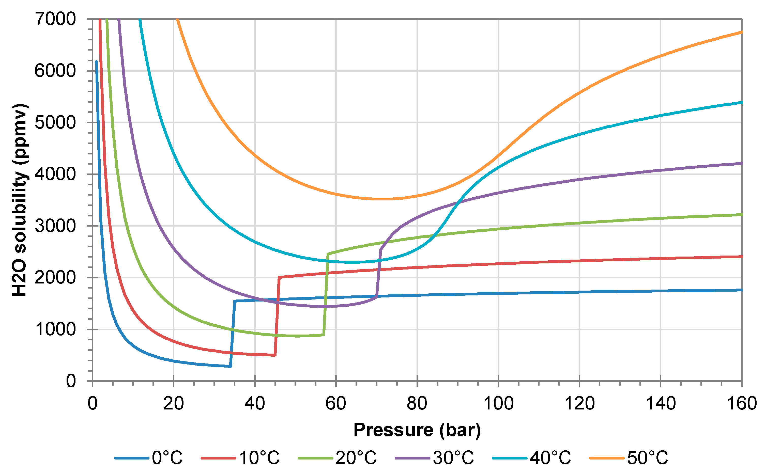
Figure 1 shows the solubility of water in pure CO
2. When CO
2 is transferred from the liquid to the gaseous state, there is a sharp drop in the water solubility, and hence there is a risk of water precipitation. The problem is enhanced by the Joule–Thomson effect, which reduces the temperature in the gas reduction valve. The reduction valves should therefore be operated with electric heating, as this prevents precipitation of liquid water. Heating will also prevent/reduce the risk of hydrate formation, which may occur at temperatures of 11 °C or lower [
16,
17]. In the gaseous state, the water solubility increases with decreasing pressure (left side of
Figure 1).
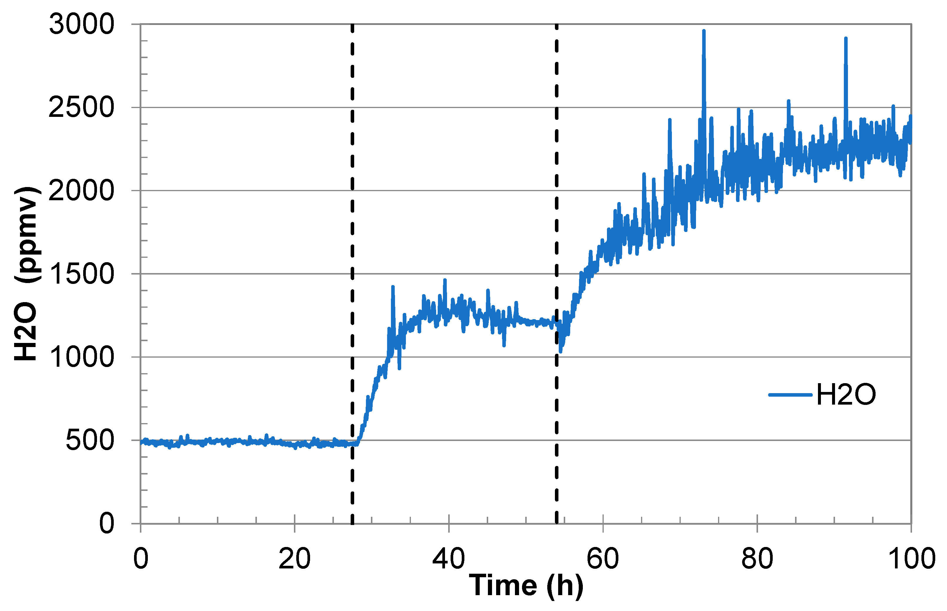
An example that shows the effect of water precipitation in the gas regulator is given in
Figure 2. The initial water analysis was very stable (500 ppmv), but it started to fluctuate somewhat when the water content was increased to 1200 ppmv. Shortly after injection of fully water-saturated CO
2 (in this example it started at 54 h), the water signal started to fluctuate significantly. This is believed to be the result of water precipitation/dissolution dynamics in the heated gas regulator. This behaviour is so common that it is used by the authors as an indication of water saturation.
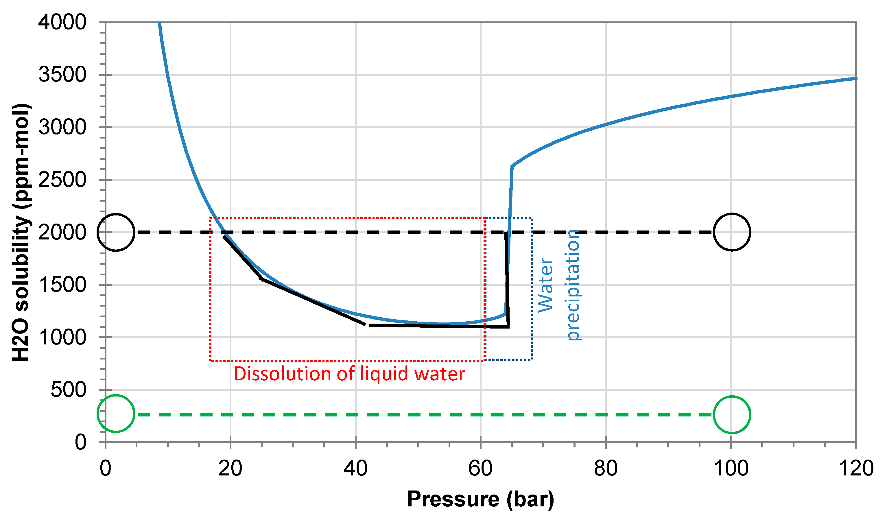
Figure 3 shows the predicted water solubility at 25 °C assuming full equilibrium and no temperature changes. If the water content is low, precipitation of water is not expected when the pressure is reduced from 100 to 1 bar (example with 250 ppmv shown by the green line/circles). The black lines/circles show the same process for a higher water content of 2000 ppmv. The water solubility is clearly exceeded during the phase transition from liquid to gaseous CO
2, where about 800 ppmv of water will precipitate as liquid water. It will gradually dissolve again when the pressure is reduced below 50 bar and it will be fully dissolved when the pressure reaches 20 bar.
A sharp drop in solubility with decreasing pressure is also observed for other species such as nitric acid, sulfuric acid, and elemental sulphur. If the precipitation is fast, species may accumulate in the heated gas regulator. This will of course result in erroneous chemical analysis, but it may also introduce clogging of the regulator, the mass flow controller, and the analysers (see the example in
Section 3.2). Furthermore, if certain species precipitate, they could introduce chemical reactions in the feeding lines from the gas regulator to the analysers. If an aqueous phase with acids precipitates inside the heated gas regulator, the water measurements may also fluctuate even in the low parts per million by volume (ppmv) range, as shown in
Section 3.3.
2.2. The Calibration Challenge
Some instruments, such as gas chromatographs, as well as UV and IR photometers, need regular calibration. Even if this process is automated, it can be a somewhat tedious process, particularly in the field. It also means that bottles with calibration gas (one for each concentration) must be available at the site and be refilled in due time. Thus, there is a technological and logistic issue that has to be dealt with. This should be manageable at a CCS facility, which nevertheless will require a certain amount of qualified work force. The situation may be different on a remote site.
2.3. Saturating the Sampling System with Analyte
Several impurities may adsorb on internal surfaces of the sampling loop, such as phase transition regulators, flow meters, and analysing lines. Normally, the volume in the sampling system should be fully replaced with CO2 feed (analyte) three to five times before a representative sample can be collected. This is not a problem for a continuous analysing system, but the lag time could be long when considering both the volume exchange and adsorption/desorption effects. This is commonly referred to as “saturating” the analysing system. If the analyte composition changes, these impurities will adsorb or desorb according to the surface equilibrium. It has been observed that H2O, H2S, and NH3 require long saturation times, while SO2, O2, and CO are much faster. The actual response time depend on the length of the analysis line and the volume and surface area of additional equipment.
One of the setups in our lab consists of 20 m 1/16′′ stainless steel tubing, three valves, two filters, a heated gas regulator, and a 300 mL autoclave. It takes about 16 h to saturate this setup when changing the water content from 5 to 1500 ppmv with 500 mL/min total gas flow. If the water content is reduced from 1500 to 1000 ppmv, stable measurements are achieved after about 2 h. The dry-up time for such a system is very long. The experience is that it takes about 2 weeks to reduce the water content from 1000 to 1 ppmv, and the last 50 ppmv are the most time consuming. It is possible to purchase tubing that has a special surface treatment (“inert tubing”) that is claimed to reduce the problem. This effect has not yet been tested by the authors.
The problem can be reduced by designing the sampling system with a high-volume exchange rate. In practice, this means low diameter tubing or a large flow of CO2. With smaller diameter tubing, there is an increased risk of clogging by solids and therefore some optimisation has to be made.
The phase transition regulator should be made of inert material. Usually, a fine tuning of the heat supply would also be necessary. More heat would at least give shorter adsorption/desorption time, but it could increase the risk of reaction between the impurities. Thus, there is a trade-off between response time and accuracy.
2.4. Sampling Location
Corrosion and impurity reactions can form solid and liquid phases [
3,
4,
5]. These products (solids, liquids) may separate from the CO
2 bulk phase due to density differences and either stick to the wall or follow the CO
2 stream. Depending on the pressure and temperature (density of CO
2), the products may be lighter or heavier than the bulk CO
2 phase. This is further complicated by the large variation of CO
2 density (varies significantly with pressure and temperature), meaning that certain components can be both lighter or heavier than the bulk CO
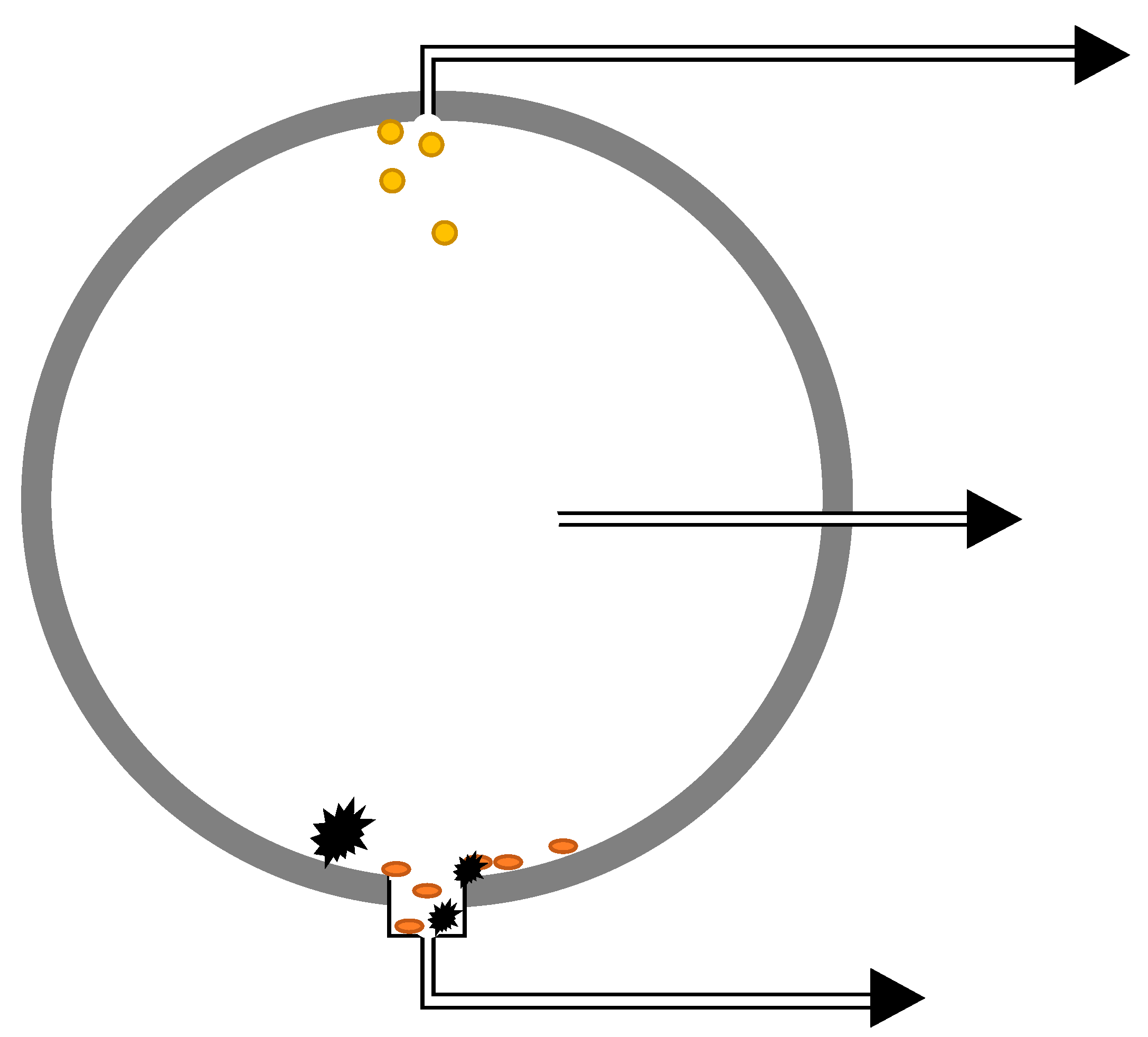
2 depending on the conditions. Flow and turbulence may also have an effect, particularly in pipelines. Products that are expected to be separated by gravity could be kept in the bulk phase as emulsions or small particles, but they may also accumulate either at the top or bottom of the transportation system. The practical sampling locations will have to be evaluated for each system, but one approach could be to sample from the top position (light components), middle position (bulk phase), and bottom position (heavy components), as indicated in
Figure 4. Applying a large-diameter flange at the bottom would allow for accumulation of heavy components if the turbulence is not too high.
Partitioning of impurities in two-phase CO
2 is the case for a number of impurities, and sampling from the gas or liquid phase will therefore give different results [
18,
19,
20]. Experiments have shown that H
2O, SO
2, and H
2S partition preferentially into liquid CO
2 phase, while O
2 partition preferentially into the gas phase. This means that it is important to carry out sampling in a manner that prevents a two-phase system, e.g., by introducing a large pressure drop by fast sampling. A piston cylinder with back pressure could be used to avoid two phase formation during analysis of a batch CO
2 sample.
2.5. Impurity Range
The impurity levels are expected to be low (typically < 10 ppmv) during normal operation, and consequently low detection limits are required. Upset conditions, on the other hand, may introduce relatively high impurity levels. Thus, there is a trade-off between wide range and accuracy of the lowest concentrations.
3. Analysis and the Need for Phase Separation
The CO
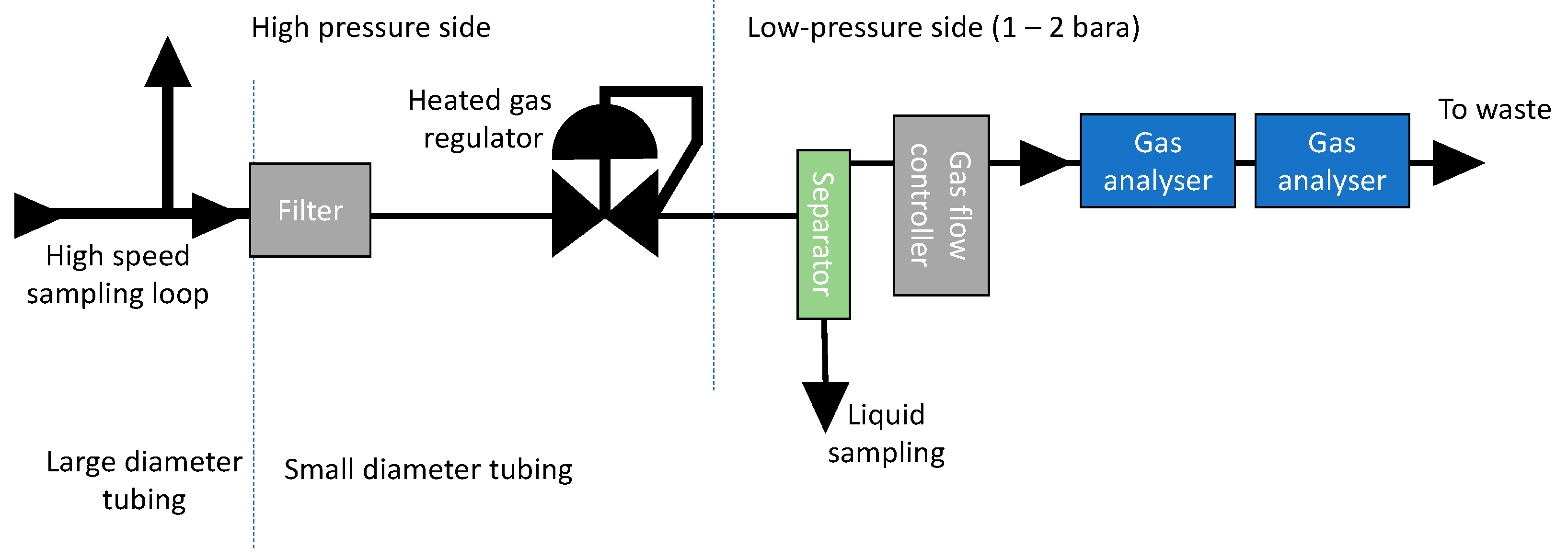
2 stream can in principle contain both gaseous, liquid, and solid products. Each of these components will usually require different types of analysing techniques and will therefore have to be separated. With gaseous components, it is here meant components that are in gaseous state around room temperature and at pressure near 1 atm (after pressure reduction). The analysing approach will probably vary from site to site, but one example of a possible solution is shown in
Figure 5.
3.1. Gasseous Species
After the heated gas regulator, the gas can be analysed directly. The choice of analysing method is usually based on a number of factors, of which economy, number of analysed species, detection limit, reproducibility, need for calibration, ease of repair/maintenance, and equipment lifetime are the most important. Analysers based on laser absorption spectroscopy were selected in the authors’ lab as the best choice due to high analysis frequency and long calibration intervals. One disadvantage with the current setup is that the number of possible analysed species is fixed. Furthermore, not all species can be analysed for (there are several reasons for this). Although this probably can be improved in the future, it means that these laser-based techniques must be combined with other analytic methods. Several laser-based analysers may also be applied in series. FTIR spectroscopy is another analytical technique that probably could be used, but at present it has not been tested by the authors. The technique is promising since it is capable of multi component analysis, and new components in principle can be added to the analysis by only changing the software.
Gas chromatography (GC) needs regular calibration, and therefore we did not use it for long-term analysis (with dense phase CO2). It is sometimes used for infrequent analysis. However, GC has the advantage that it relatively easy can be modified to analyse for new species.
Regardless of the analysis technique, it is difficult to find one technique and instrument that can handle all species, and thus several analysers have to be used in combination.
3.2. Solids
Solids can be separated from the bulk CO2 phase with filters. Since the solubility of certain components vary with pressure, it is best to apply the filter before the phase transition regulator. This will also prevent clogging problems of the gas regulator. Nevertheless, the filter housing must be able to handle the CO2 pressure, and it must withstand frequent depressurization in a controlled manner (particularly soft materials such as rubber gaskets or Teflon-coated diaphragm can be damaged due to rapid depressurisation). The filters could be analysed by standard methods, e.g., by X-ray powder diffraction (XRD), scanning electron microscopy (SEM), and energy-dispersive X-ray spectroscopy (EDS). Dissolving the products in a suitable solvent could be another solution.
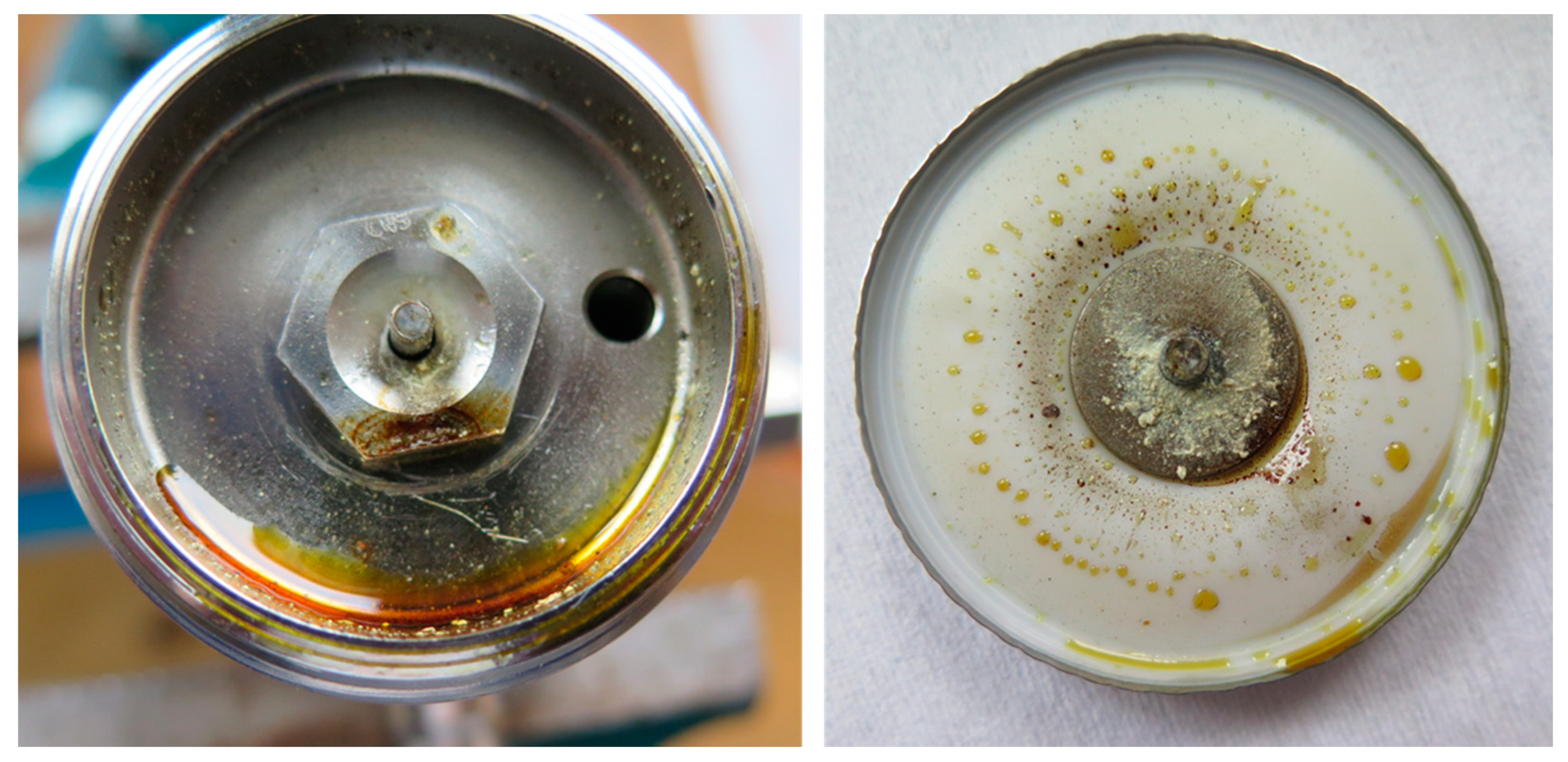
A filter can also be installed on the low-pressure side for protection of the analysers and the mass flow controllers, etc. Comparison of filters from up- and downstream the reduction valve may provide useful information, since the pressure drop over the heated gas regulator may lead to precipitation of certain species (see
Figure 6). Previous research [
3,
10,
15] has shown that interaction between impurities may occur when certain types are present, and the concentrations exceed a critical limit. The analysis system is vulnerable to precipitation of solids if they settle inside the analytical instruments. The green/yellow solids seen in
Figure 6 (diaphragm to the right) was identified with XRD to be elemental sulphur. The sulphur was initially fully dissolved in the CO
2 stream not transported to the gas regulator as solid but rather as dissolved species [
10] in the CO
2 and precipitated when the pressure dropped over the regulator. This is commonly observed, and most of the impurity solubilities shows a minimum solubility right before the phase transmission from gas to liquid (see an example in
Figure 1). As long as such species remain dissolved in the CO
2 stream, they might not be a problem for the transport system, but it may introduce problems for the analysing loop.
3.3. Liquids
Liquids can be difficult to separate from dense phase CO2 since they may have almost the same density. The density differences are much higher downstream the pressure regulator (where CO2 is in the gaseous state), and gaseous and liquid species can then be separated by top and bottom streams in a small separator. The separator could even be equipped with a small window for in situ observation of liquids. The liquid could be analysed using conventional method, such as ion chromatography, liquid chromatography, etc.
Even if there is no separate liquid phase in the CO
2 stream, liquids may condense inside the heated regulator due to the pressure drop, as shown in
Figure 6. An ion chromatograph analysis of the liquid in
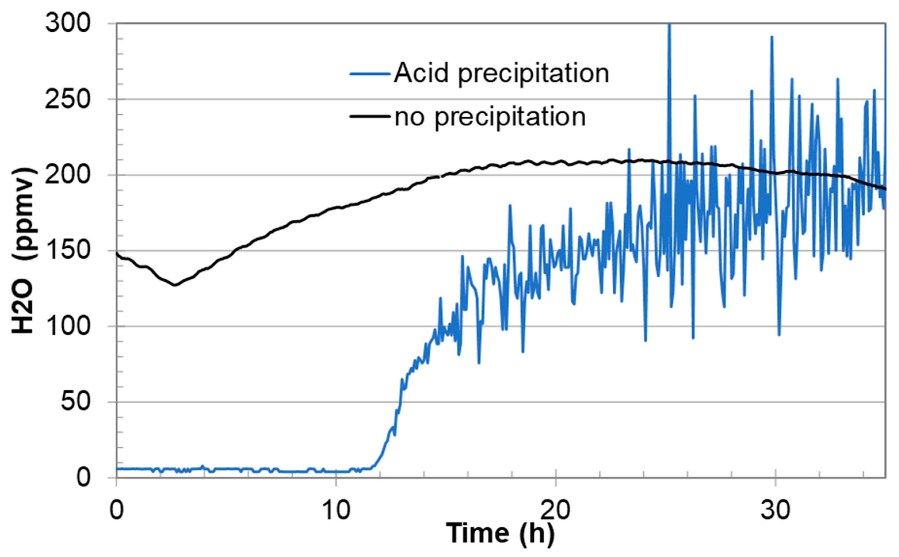
Figure 6 showed that it consisted of both nitric and sulphuric acid. Installation of a drain on the regulator would allow for sampling of such liquids while at the same time providing a simple method for purging the regulator for liquids and particles. It is expected that routine purging would decrease the need for maintenance due to corrosion of the regulator material and solid accumulation. It may also improve the chemical analysis. Typical signs of liquid condensation inside or downstream the regulator are fluctuations in the water analysis, as shown in the example in
Figure 7.
4. Monitoring Multiple CO2 Streams
For single CO2 streams, it should be relatively straightforward to document that the quality is within a given specification by using the earlier mention techniques. If no reaction or corrosion occurs, the content of impurities should be the same along the whole transport system. Changes in impurity concentration would indicate that chemical reactions or even corrosion is taking place. This will obviously require multiple analysing points.
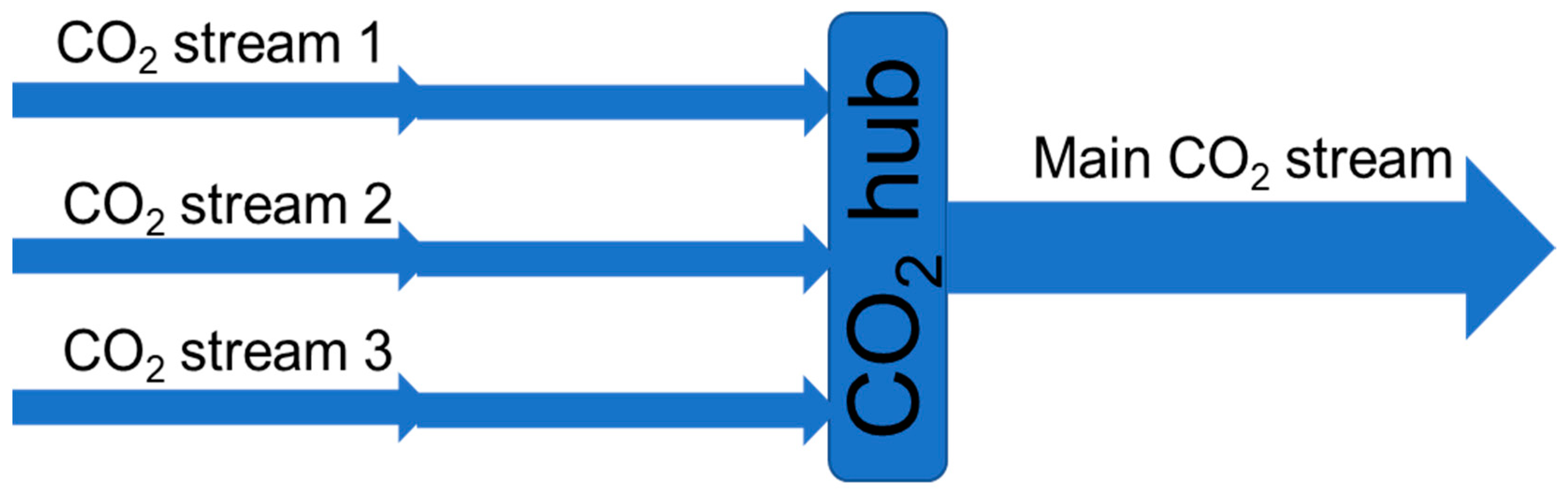
For a large CO
2 transportation network, there will be CO
2 streams from several CO
2 sources gathered in large transport lines or temporary stored for ship transport (see the illustration in
Figure 8). The different CO
2 streams might have different impurities in both type and concentration. Even if these streams are stable individually (no chemical reactions), chemical reactions could occur when the streams are mixed. Thus, there is a need to document the impurity content before and after mixing.
4.1. Reactions
Due to the large number of possible impurities, the number of possible chemical reactions is high. The most important reactions that were identified in the Kjeller dense phase CO
2 project (KDC) [
3,
4,
9,
15,
21] were
Nitrogen dioxide is a strong oxidation agent and will readily react with hydrogen sulphide to sulphur dioxide and water (reaction (1)). As long as oxygen is present, nitrogen dioxide will be regenerated according to reaction (2). It should be noted that due to this regeneration, only trace amount of NO2 is required to oxidise H2S as long as oxygen is present. The only NO2 sink will be formation of nitric acid or corrosion.
Sulphuric acid is formed according to reaction (3), but to form liquid acid inside the transport system, it has been observed that the SO2 content needs to exceed 50–60 ppmv before H2SO4 forms and precipitates as a liquid phase (25 °C and 100 bar).
Reactions (1)–(4) could be used for guidance when interpreting the results from the analyses of the CO2 streams. This will be discussed further in the following chapters.
4.2. False Accordance with the Specification
Monitoring the composition of a CO
2 stream where the impurities may react before the analysis introduces the need for special evaluations in addition to the chemical analysis. For example, monitoring parameters such as flow, pressure, and temperature could reveal possible risk of precipitation (see, for example,
Figure 3). Comparison of analyses at different positions can also provide valuable information. All of this should be combined and compared with the known chemical reactions and limits (see
Section 4.1) and also compared to thermodynamic models (if available).
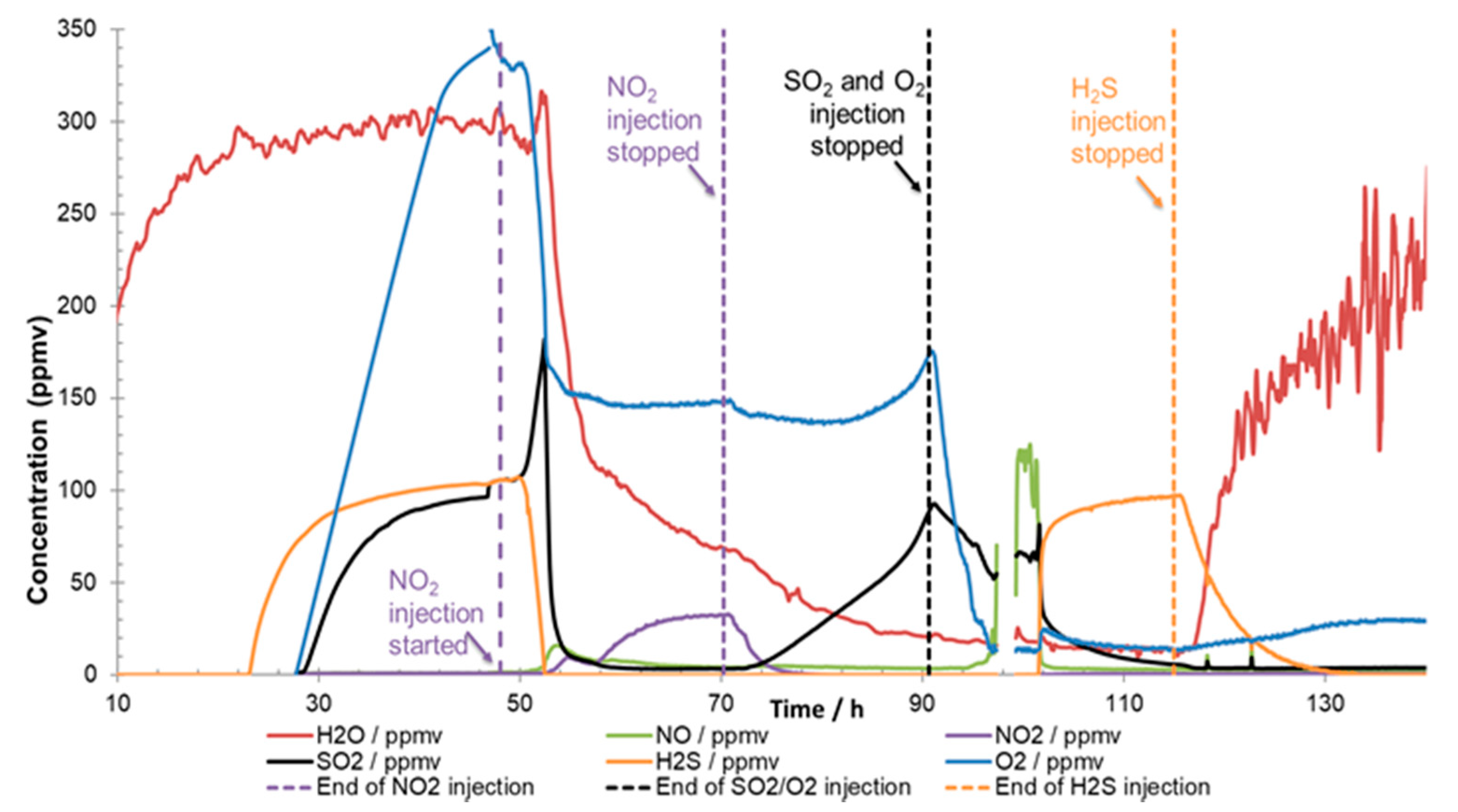
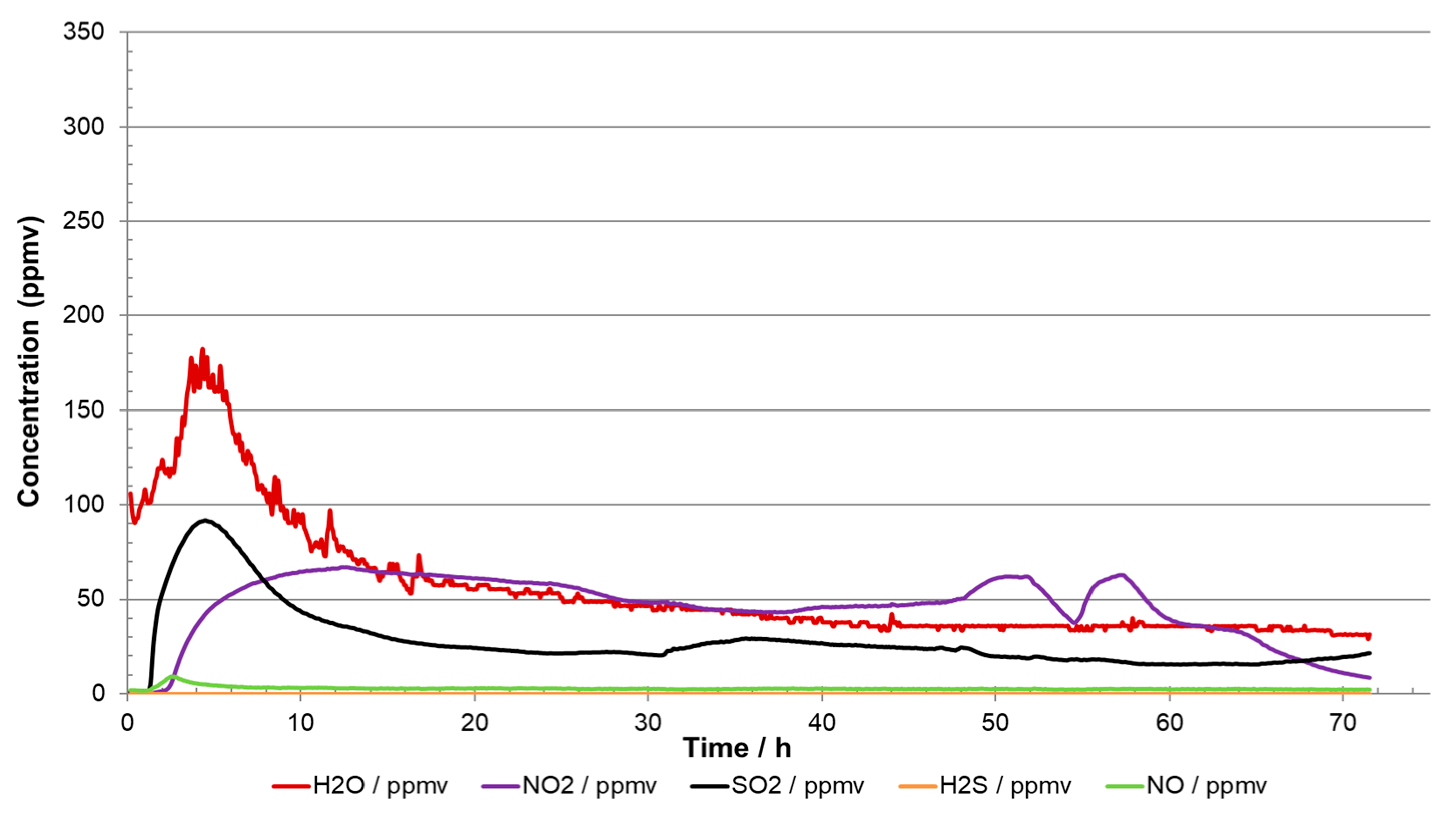
Examples of how misleading the analyses can be are shown in
Figure 9 and
Figure 10. The injected impurity concentrations were the same in both experiments [
9] but the injections of the impurities were started at different times. In
Figure 9, it is quite clear that no chemical reactions took place when H
2O, SO
2, O
2, and H
2S were injected as they all reached stable target values. Once the NO
2 injection started, reactions took place, and an aqueous phase of H
2SO
4 and HNO
3 precipitated. In the other experiment (
Figure 10), where all the impurities were injected simultaneously from start-up, the analysis showed practically zero content of H
2S, and SO
2 and O
2 were much lower than the injected content. The readings in
Figure 9 could therefore erroneously lead to the conclusion that the CO
2 stream was in accordance with the specification, even if more than 70 percent of the impurities were missing due to reactions. The reason for the missing impurities was reaction to acids (reactions (3) and (4)) and solid formation. If all the sulphur species (SO
2 + H
2S) react to sulphuric acid (reaction (1) + reaction (3)), about 500 g would be produced per ton CO
2. A system transporting 1 megaton per year would in this case produce 500 tonnes of acid per year. This large amount of acid would most likely threaten the integrity of the transportation system due to corrosion, and routines must be implemented to prevent (and detect) such a situation. This emphasises the importance of several measuring points to ensure sufficient control over the transport system, and the design of the analysing system must take into consideration that new products from chemical reactions could appear in addition to those impurities included in the specification.
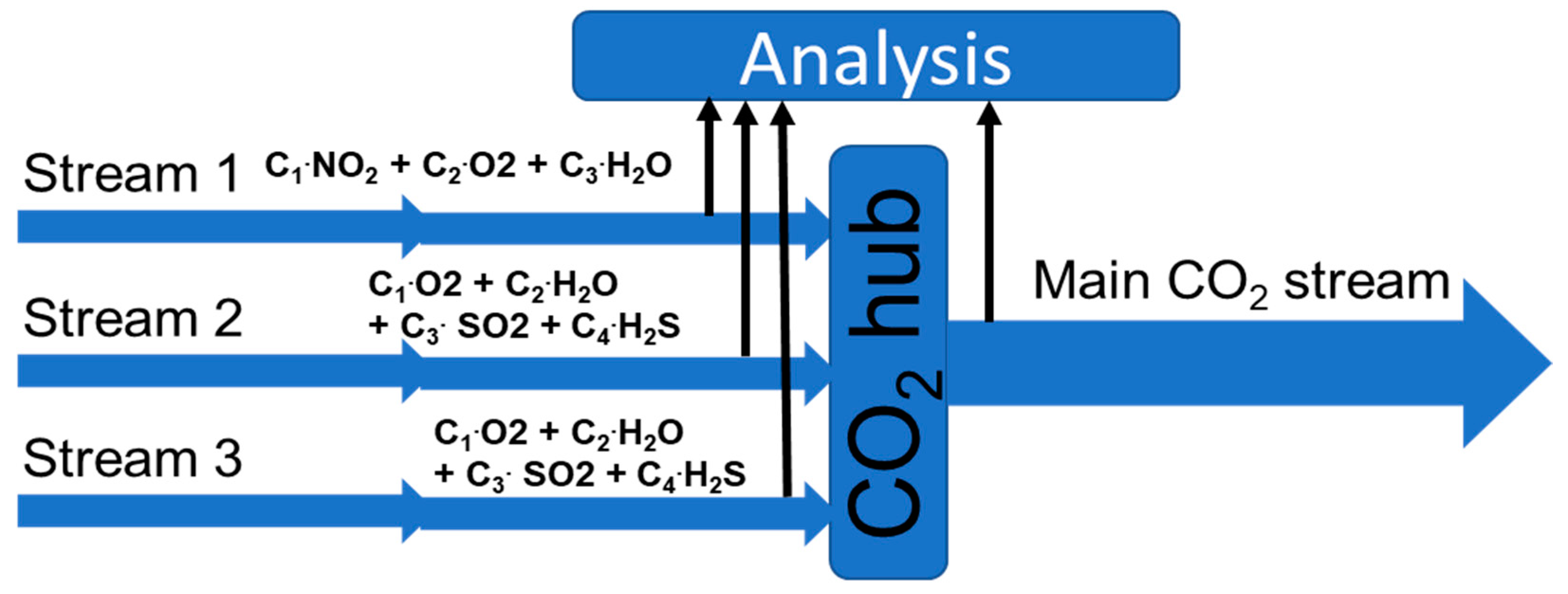
4.3. Simulation and Predicting
By using reactions (1) to (4), we were able to make simple predictions of the results of mixing CO
2 streams. If all side streams and the main CO
2 stream (
Figure 11) are monitored, it is possible to identify upsets. If no reactions take place, a simple mass balance of the small streams should give the composition of the mixed stream.
However, even if most of the chemical reactions are known, a full simulation of the mixing of multiple CO2 streams with occurring reactions is quite a complex process. Parameters such as chemical kinetics and competition between reactions, surface adsorption, and catalysing effects are not fully understood at present. Another aspect that would add complexity to the simulation occurs if a separate aqueous phase forms and accumulate in the system. The presence of an aqueous phase might not only change the kinetical parameters but could also change the ongoing reactions or introduce new reactions, including corrosion reactions, that would further complicate the simulation.
The results from the KDC-project are currently being implemented in a thermodynamic model developed by OLI Systems [
22,
23]. The model is still in the development stage for use in CCS systems.
Even though an accurate simulation might be complex, the prediction from the reaction alone would give valuable input to the outcome of mixing streams or building specifications.
Table 1 shows an example of such prediction, where no aqueous phase will form since the sum of H
2S and SO
2 is well below the threshold value for reaction (3) (see
Section 4.1). An interesting outcome of the exercises is that reaction 1 leads to higher concentration of SO
2 and H
2O, which in certain situations could exceed the threshold for reaction (3), even if the original SO
2 content was well below this level. Further increase of impurity content could eventually result in exceeding the accepted specification. Yet, research has shown that the concentrations in
Table 1 are safe [
3].
The understanding of ongoing processes in the transported CO2 might ease the simulations but it might also untangle the complex analysis after mixing several CO2 streams loaded with even more types of impurities.
5. Conclusions
Analysis of impurities in dense phase CO2 streams requires pressure reduction and phase transformation to gaseous CO2 and is therefore more complicated than analysis of gaseous CO2 alone. Possible reactions of impurities make such analysis even more challenging, particularly since even 99.95% pure CO2 (food grade) has the potential to produce acids and solids, which may have negative effects on the analysis system. Impurities may partition between phases, and this may be another complicating factor during analysis. Precipitation of solids and liquids on the low-pressure side of the analysis line may also introduce challenges due to particle accumulation, corrosion, and fluctuation of certain impurities that interact with the liquids.
Multiple analysing points along the CO2 transportation system (e.g., inlet and outlet) will increase the possibility to reveal ongoing processes such as chemical reactions and/or corrosion. If multiple CO2 streams are being merged in a network, it might be necessary to analyse all CO2 streams before and after mixing in order to ensure that the specification is fulfilled. Such analysis could also be assisted by predictions based on identified chemical reactions.


