Joint Modelling of Wave Energy Flux and Wave Direction

Abstract

In the context of wave resource assessment, the description of wave climate is usually confined to significant wave height and energy period. However, the accurate joint description of both linear and directional wave energy characteristics is essential for the proper and detailed optimization of wave energy converters. In this work, the joint probabilistic description of wave energy flux and wave direction is performed and evaluated. Parametric univariate models are implemented for the description of wave energy flux and wave direction. For wave energy flux, conventional, and mixture distributions are examined while for wave direction proven and efficient finite mixtures of von Mises distributions are used. The bivariate modelling is based on the implementation of the Johnson–Wehrly model. The examined models are applied on long-term measured wave data at three offshore locations in Greece and hindcast numerical wave model data at three locations in the western Mediterranean, the North Sea, and the North Atlantic Ocean. A global criterion that combines five individual goodness-of-fit criteria into a single expression is used to evaluate the performance of bivariate models. From the optimum bivariate model, the expected wave energy flux as function of wave direction and the distribution of wave energy flux for the mean and most probable wave directions are also obtained.

1. Introduction

Marine renewable energy applications (especially, offshore wind, wave, and current/tide) are gaining ground as means for deriving electrical power due to the commitment of the EU member states to reduce pollutant emissions by substituting fossil fuels with clean energy sources [1,2]. To date, EU funds have supported particularly the wave energy sector with respect to technology R&D. Although the technological progress is remarkable with numerous design concepts and prototypes to harness energy from sea waves, the corresponding commercial stage follows a slower pace.

The particular advantages of wave energy (e.g., high energy density, small energy loss, predictability) render its exploitation promising not only in areas with high wave energy flux like the Atlantic Ocean but also in areas with relatively calm wave climate and thus with intermediate levels of power availability, like the Mediterranean Sea; see, for example, [1,3,4]. Usually, the later areas are characterized by low variability achieving better survivability, without increase of capital expenditure [5]. In order to make wave energy production feasible and economically viable, it is necessary, among others, to deploy wave energy converters (WECs) based on the accurate knowledge of the wave climate and its temporal variability in the area of interest [6]. The wave climate variability is also responsible to a great extent for the uncertainty in electricity production of a wave energy project, an aspect that has been studied by [7,8].

The local wave resource assessment can be based on buoy measurements, reanalysis results, and satellite altimetry data commonly through spectral analysis. See also [9,10,11,12,13,14]. Such studies are usually confined in the statistical description of particular wave spectral parameters, such as significant wave height $H_S$ defined as $H_S\cong 4\sqrt{m_0}$; energy period $T_e$, $T_e=m_{-1}/m_0$; and mean wave direction ${\Theta }_W={\tan }^{-1}\left(\frac{\iint S_{\eta \eta }\left(f,\theta \right)\sin \theta d\theta df}{\iint S_{\eta \eta }\left(f,\theta \right)\cos \theta d\theta df}\right)$, where $m_n={\int }_0^{\infty }{f}^n{S}_{\eta \eta }\left(f\right)df$, $n=\cdots ,-2,-1,0,1,\cdots$, is the $n$—order spectral moment, $S_{\eta \eta }\left(f\right)$ is the spectral density function, and $f$ is the spectral frequency; see, e.g., [15]. However, there are recent studies on wave energy resource characterization [16] that are based on the six IEC parameters, which include at least two directional parameters: direction of maximum energy and directionality coefficient.

Wave energy flux per unit length of wave front ($W/m$), which is also known as wave power density or wave energy potential, can be evaluated from the following relation:

$$P_W=\rho g{\int }_0^{2\pi }{\int }_0^{\infty }{c}_g\left(f,d\right)S_{\eta \eta }\left(f,\theta \right)dfd\theta ,$$

(1)

where $\rho$ is the density of seawater, $g$ is the acceleration of gravity, $c_g\left(f,d\right)$ is the group velocity, $d$ is the water depth, and $\theta$ is the direction of wave propagation; see also [17,18]. For deep water, the above relation for the total wave energy flux is simplified as follows:

$$P_W=\frac{\rho g^2}{4\pi }{\int }_0^{\infty }\frac{1}{f}{S}_{\eta \eta }\left(f\right)df,$$

(2)

which is usually expressed through $H_S$ and $T_e$ via the following relation:

$$P=\rho g^2\frac{H_S^2{T}_e}{64\pi }\cong 0.49H_S^2{T}_e \left(\mathrm{in} kW/m\right),$$

(3)

where $\rho =1025 kg/m^3$ and $g=9.8066 m/s^2$.

In the framework of wave resource assessment studies, data validation, variability and uncertainty measures, and analysis of extreme waves should also be included. See, e.g., [4,19,20,21,22,23,24].

Regarding wave climate analysis per se, a lot of work has been done for the modelling of $H_S$ and $T_e$ (or spectral peak period $T_P$ and mean zero-up crossing period ${\overline{T}}_Z$). Among the most common probability distributions for modelling $H_S$ (and/or $T_e$/$T_P$/${\overline{T}}_Z$) are the Beta, the Gamma, the Generalized Gamma, the Weibull, and the Lognormal distributions, with the latter one being the most widely used. An alternative modelling approach is non-parametric methods; in this context, kernel density estimation is frequently applied. Essentially, the kernel is used as a weighting function centred at the data points and its extension (around the data points) is defined by a smoothing parameter. Some standard reference books for non-parametric estimation are [25,26].

However, the univariate models are not sufficient in the context of a detailed long-term analysis, especially with respect to design purposes, load calculations, and reliability analyses; thus, the bivariate description of the above-mentioned wave parameters is necessary; [27,28,29]. Different approaches have been presented for the joint description of wave height and period. For instance, parametric bivariate distributions, conditional-distribution approach, kernel-based models, and copula-based models as well, provide alternative probabilistic description of these variables; see, e.g., [27,30,31,32]. Furthermore, [33,34] have provided distributions for the joint description of wave power–wave height and wave power–wave period for individual waves, an approach that is complementary in long-term analysis of the wave climate at a particular site.

WECs can be classified regarding their direction of orientation (and size) into three categories: attenuators, point absorbers, and terminators; see, e.g., [35]. Unlike a point absorber that converts energy from waves coming from all directions, attenuators and terminators should be elongated parallel and perpendicular to the propagation of wave direction, respectively, to yield high-energy conversion efficiency. This sensitivity to directionality affects the standard deviation of the capture length (i.e., ratio of the WEC power output to the sea state power) of WECs as has been demonstrated by [8]. Moreover, as is emphasized in [36], apart from $H_S$ and $T_e$, the performance of a WEC should be based on additional attributes of the sea state including variability of mean wave direction, directional spread and spectral shape, and that the uncertainties of the performance results of the WECs can be reduced if these dependencies are explored and quantified; see also [37]. In the same context, [38] highlighted that developers of WECs should provide information regarding the effects of wave direction on the performance of WECs for an accurate assessment of wave energy since it affects wave propagation and in turn, the distribution of wave resource. A similar suggestion has been provided earlier by [36], advising to provide power matrix for different mean wave directions with the related uncertainty matrix. Reference [7] also has noted that vicinal sites characterized by similar resource levels may exhibit differences in acquirable wave energy with time due to the varying wave directional exposure.

The importance of analysing wave direction for performance optimization purposes of a WEC, and generally, in wave energy studies, has been also emphasized in [39,40]. In [41], variability of wave heights and wave power has been assessed with respect to wave direction for a more realistic wave resource analysis at different locations in the southwest UK. The directional dependence of wave height and, consequently, wave energy generation was more than evident. The authors concluded that site selection for commercial development of wave energy, reduction of grid integration hindrances, and increase of power smoothing are highly dependent on directional exposure of sites. Reference [42] has assessed wave power and its temporal variability for various water depths off the central west coast of India and examined the directional distribution of wave power at shallower water depths. Reference [43] has highlighted the wave (and wind) directionality effects on offshore wind turbines, supported by a jacket structure during hurricane events, while [44,45] have stressed the significance of wave direction, among others, that may lead to larger fatigue damage for certain platforms under specific conditions. Overall, the accurate description of wave directional characteristics and their variability is important when assessing wave energy potential at a site; see, e.g., [46], while wave direction affects significantly wave propagation, and in turn, wave resource distribution, in an area.

In this work, instead of modelling the involved individual random variables in wave energy assessment studies, i.e., significant wave height $H_S$, energy period $T_e$, and mean wave direction ${\Theta }_W$ (${\Theta }_W$ is subsequently denoted as $\Theta$), the joint assessment of “wave energy flux $P$” and “mean wave direction $\Theta$” is performed. To the authors’ knowledge, the joint description of $P$ and $\Theta$ has not been presented yet, although it is of high importance for the emerging wave energy sector and relevant wave resource analysis applications. Moreover, some straightforward applications derived from the proposed methodology are also presented.

In this framework, numerous univariate conventional and mixture parametric models have been addressed with respect to the (linear) variable $P$. The directional variable $\Theta$ is adequately described through a finite mixture of the von Mises distribution that has already proven to be efficient in this case [40,47,48]. The construction of the bivariate distribution functions for ($P,\Theta$) is accomplished through the Johnson–Wehrly (JW) parametric model. An important feature of the JW model is that its density functions rely on the corresponding univariate marginal distributions while an additional parameter quantifies the correlation/dependence of the linear and directional variable. A detailed evaluation of the resulting bivariate distributions is made by applying five bin-defined metrics, namely, adjusted coefficient of determination, index of agreement, mean absolute error, root mean square error, and ${\chi }^2$ statistic, as well as a synthetic criterion that combines the above criteria into a single expression. See also [47,49,50].

The structure of the present work is the following: in Section 2, wave data obtained from three buoy locations in the Greek Seas along with data from numerical wave models in three locations (Gulf of Lion, Gulf of Biscay, and North Sea) are described, and a preliminary statistical analysis is performed for wave energy flux $P$ and mean wave direction $\Theta$ (subsequently referred to as simply wave direction). The examined univariate probability models for $P$ and $\Theta$ are presented in Section 3. Specifically, for the parametric modelling of wave energy flux, several conventional and mixture distributions are applied while wave direction is modelled by using a finite mixture of the von Mises distribution. The bivariate JW probability model is briefly presented in Section 4. Section 5 deals with the statistical criteria used to evaluate the performance of both univariate and bivariate models. Based on the goodness-of-fit evaluation criteria, the derived bivariate models are compared, and the corresponding results are discussed in Section 6. In Section 7, the best bivariate model for ($P,\Theta$) for each examined area is implemented to provide analytic results that could be used in feasibility studies regarding wave farm development in the corresponding areas. The last section includes the concluding remarks of this analysis.

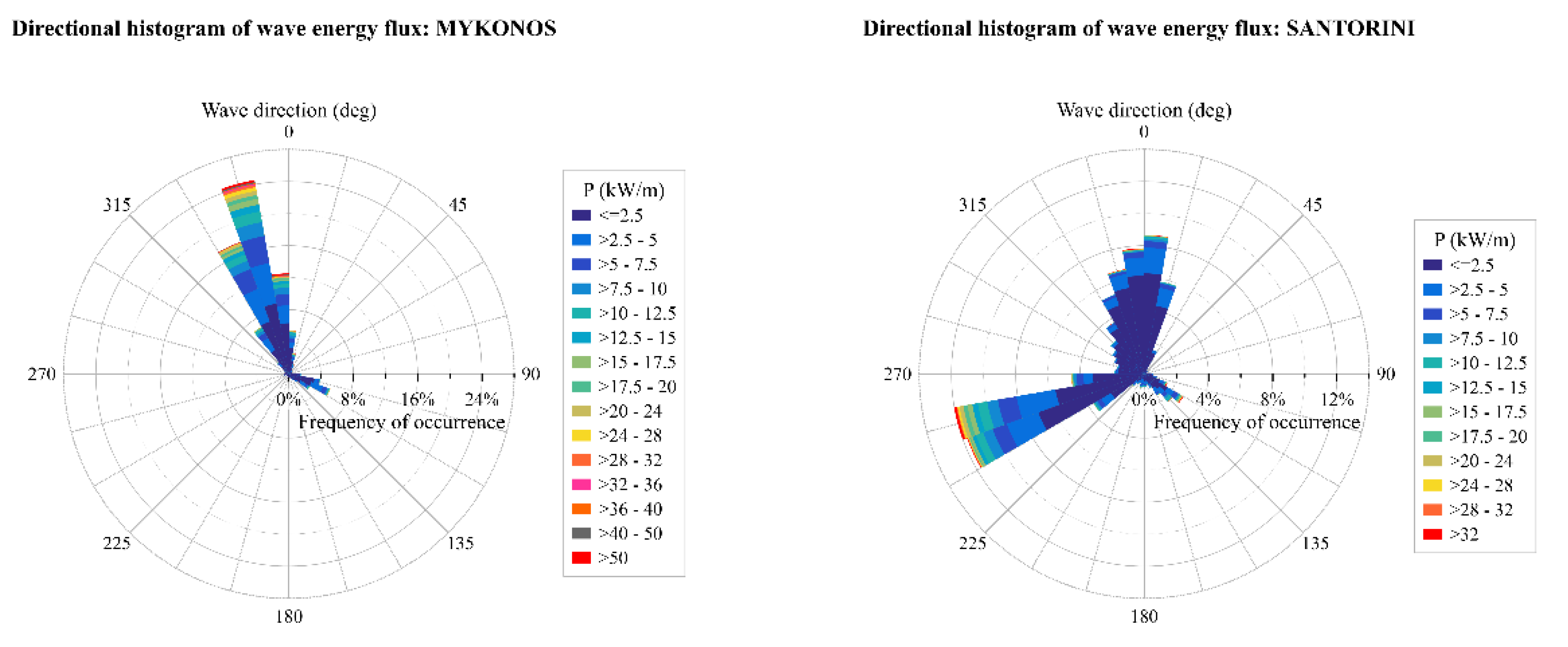
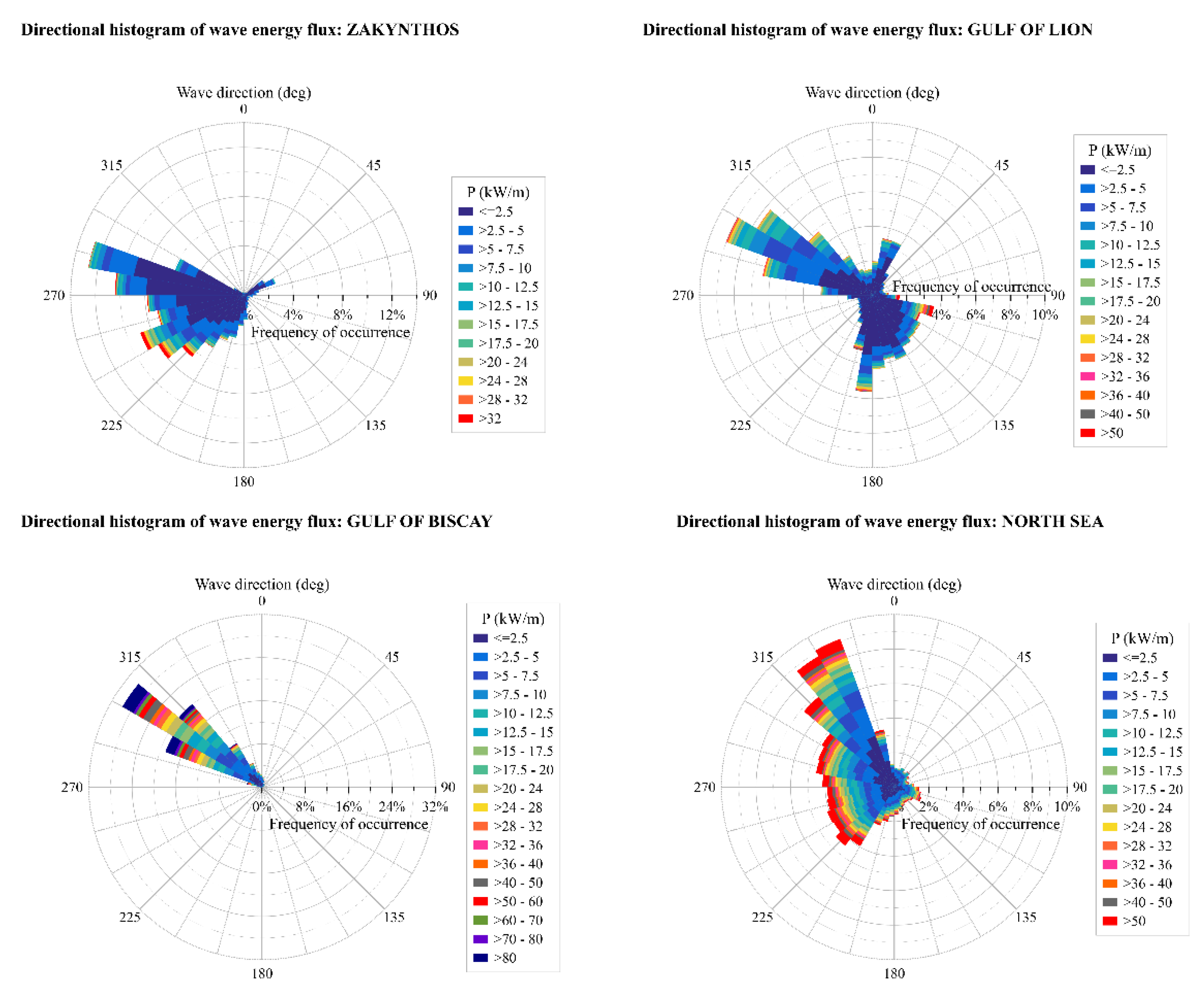
2. Description of Wave Data

Three different sources of wave data have been used in this work, corresponding in offshore areas with different wave characteristics and in turn, wave climate. The first source is in situ wave data from the Greek Seas (Aegean and Ionian seas), obtained from three oceanographic buoys of the POSEIDON marine monitoring network [51,52]. Wave measurements from buoys are confined in the Greek Seas as this data source was available to the authors. The wave parameters that were obtained were the significant wave height $H_S$ and the energy period $T_e$ in order to estimate wave energy flux $P$, and the wave direction $\Theta$. The geographical coordinates, the measurement period, the sample size, and the water depth for each buoy location are listed in

Table 1. Location names, geographical coordinates, observation periods, sample size, and depth of wave data sets.

Location Name	Latitude, Longitude (°)	Observation Period	Sample Size	Depth (m)
Mykonos	37.51° N, 25.46° E	2007–2010	7406	−92
Santorini	36.25° N, 25.49° E	2007–2010	8613	−342
Zakynthos	37.85° N, 20.36° E	2007–2010	5002	−2,072
Gulf of Lion	42.98° N, 4.00° E	2006–2010	14,364	−95
Gulf of Biscay	43.60° Ν, 3.00 W	2006–2010	14,364	−288
North Sea	56.25° N, 5.62° E	2006–2010	14,608	−48

; see also Figure 1. The wave data were firstly filtered while only concurrent wave measurements of the three parameters ($H_S$, $T_e$, and ${\Theta }_W$) were taken into consideration.

Furthermore, wave data obtained from numerical wave models were also analysed. The first numerical wave model data set is produced by the Mediterranean Sea Waves forecasting system, i.e., a wave model that is based on WAM Cycle 4.5.4 and is provided by the EU Copernicus service [53] with spatial resolution 0.042° × 0.042°. The selected grid points correspond to locations in the gulfs of Lion (France) and Biscay (Spain). The second wave data set is obtained from the ERA20C reanalysis product of the European Centre for Medium-Range Weather Forecasts (ECMWF), available at 1.25° horizontal spatial resolution. Ocean waves are described by spectra on 25 frequencies and 12 directions [54]. The selected grid point corresponds to a location offshore southern Norway, in the North Sea. All the spectral parameter time series (defined in Section 1) that are analysed in the present work have a 3-h step. See also Table 1 and Figure 1. More details and discussion as regards spatial distribution of wave spectral parameters, numerical wave models, and their validation through field data can be found for example in [55,56,57].

The following linear and directional parameters are necessary for the computations regarding the probability density functions presented in Section 3 and Section 4. Specifically, the statistical parameters of wave energy flux $P$, i.e., mean ${\mu }_P$, median $P_{0.5}$ and maximum values $ma{x}_P$, standard deviation ${\sigma }_P$, and coefficient of variation $C{V}_P={\sigma }_P/{\mu }_P$, where ${\mu }_P$ is the mean value of $P$, skewness $Sk$, and kurtosis $Ku$ are presented in

Table 2. Basic linear statistics of wave energy flux at the examined locations.

Location Name	${\mathit{\mu }}_{\mathit{P}}$ kW/m	${\mathit{P}}_{0.5}$ kW/m	$\mathit{m}\mathit{a}{\mathit{x}}_{\mathit{P}}$ kW/m	${\mathit{\sigma }}_{\mathit{P}}$ kW/m	$\mathit{C}{\mathit{V}}_{\mathit{P}}$ %	$\mathit{S}\mathit{k}$	$\mathit{K}\mathit{u}$
Mykonos	4.634	2.136	135.961	8.031	173.31	6.155	60.025
Santorini	2.852	1.350	96.760	4.807	168.536	6.138	63.977
Zakynthos	3.720	1.567	101.183	6.747	181.389	5.870	53.964
Gulf of Lion	4.587	1.605	224.762	9.185	200.229	8.436	127.003
Gulf of Biscay	20.652	8.506	612.400	37.290	180.569	5.210	41.049
North Sea	14.465	5.801	491.759	25.340	175.184	4.975	42.137

. For the measured data, the highest mean, median, maximum, standard deviation, and skewness values are recorded at Mykonos, and for the model wave data, the highest values for median, maximum, and standard deviation are encountered at Gulf of Biscay. Gulf of Lion exhibits by far the highest $C{V}_P$, skewness, and kurtosis values. Clearly, the most energetic wave climate from the examined locations is encountered in the Gulf of Biscay.

In

Table 3. Basic circular statistics of mean wave direction at the examined locations.

Location Name	${\mathit{m}}_{\mathit{\Theta }}$ deg	${\mathit{\Theta }}_{0.5}$ deg	${\overline{\mathit{R}}}_{\mathit{\Theta }}$	${\mathit{V}}_{\mathit{\Theta }}$	${\mathit{s}}_{\mathit{\Theta }}$
Mykonos	353.65	76.07	0.595	0.405	0.900
Santorini	301.31	285.82	0.407	0.593	1.089
Zakynthos	249.69	253.96	0.628	0.372	0.862
Gulf of Lion	256.89	285.60	0.130	0.870	1.319
Gulf of Biscay	312.98	308.49	0.904	0.096	0.439
North Sea	286.93	294.99	0.415	0.585	1.081

, the values of the main circular statistical parameters (i.e., mean direction $m_{\Theta }$, median direction ${\Theta }_{0.5}$ (its interpretation is analogous to the classic median), mean resultant length ${\overline{R}}_{\Theta }$ (that quantifies the spread of the variable), circular variance $V_{\Theta }=1-{\overline{R}}_{\Theta }$, and circular standard deviation $s_{\Theta }=\sqrt{-2\ln {\overline{R}}_{\Theta }}$, as regards wave direction $\Theta$) are presented. The definitions of the above parameters can be found in [58]. The mean wave direction at Zakynthos and Gulf of Lion is coming from the WSW sector, at Santorini and Gulf of Biscay from NW, at Mykonos from the NNW sector, and at the North Sea location from the WNW sector. Moreover, the highest and the lowest values of ${\overline{R}}_{\Theta }$ are encountered in Gulf of Biscay (0.904) and Gulf of Lion (0.130), respectively, while the corresponding values for $V_{\Theta }$ can be found in Gulf of Lion (0.870) and Gulf of Biscay (0.096). The value of $V_{\Theta }$ for Gulf of Lion, which is close to 1, denotes that the range of the corresponding directions is wide while the value of ${\overline{R}}_{\Theta }$ for Gulf of Biscay reveals a small dispersion of the data.

In Figure 2, the directional histograms of wave energy flux are presented for the examined locations.

3. Univariate Probability Models for Linear and Directional Variables

3.1. Parametric Models for Linear Variables

Since there is no theoretical justification for adopting a particular probability distribution for wave energy flux, several distributions are implemented according to specific goodness-of-fit tests. The initial evaluation criteria are based on the performance of two goodness-of-fit tests, the Kolmogorov–Smirnov (K-S) and the Anderson–Darling (A-D) tests that were calculated for 24 conventional distributions for the modelling of $P$; see also [47,59,60]. The examined distributions are the following:

(1)

Two-parameter cdfs: Exponential, Gaussian, Rayleigh;

(2)

Three-parameter cdfs: Erlang, Error, Fatigue Life, Fréchet, Gamma, Generalized Extreme Value, Generalized Logistic, Generalized Pareto, Inverse Gaussian, Log-Logistic, Lognormal, Log-Pearson 3, Pearson 5, Weibull;

(3)

Four-parameter cdfs: Beta, Burr, Dagum, Generalized Gamma, Johnson S_B, Kumaraswamy, Pearson 6.

The two- and three-parameter pdfs determine the first, second, and third moments of the distribution (i.e., mean value and variance, and skewness), respectively, while the pdfs with four parameters represent additionally kurtosis (fourth moment). Typically, as the number of parameters increases, the distributions tend to be more robust and can provide a better representation of the data. However, distributions with small number of parameters can be more straightforward as regards their definition and use in applications.

Then, the ten distributions that provided the smallest statistic values of K-S and A-D tests were selected for each examined location. Due to several overlaps between the examined locations and the two tests, the total number of the fitted distributions with a good performance was relatively small; see also Section 6.1. The distributions that proceeded to the next step of evaluation are the following: Burr (BUR), Dagum (DAG), Lognormal (LGN), Fatigue Life (FAL), Pearson 6 (PE6), Log-Logistic (LGL), and Generalized Gamma (GNG). In the Appendix A, the analytic forms of the above-mentioned probability density functions (pdfs) are provided. Moreover, four parametric mixture distributions are also considered: one homogeneous, the Weibull (WW) mixture distribution, and three inhomogeneous, the 2-parameter Weibull–GEV (WGEV), the Exponential–Lognormal (ELGN), and the Exponential–Weibull (EW) mixtures. For the definition of these mixture distributions, see the Appendix A. The parametric mixture distributions were selected due to their suitability in describing right-skewed data and were not considered in the evaluation of the rest conventional distributions by means of K-S and A-D tests. The selected mixture distributions are characterized by rather large values of $R_{a,1}^2$ ($\ge 0.99$). See also Section 5.1.

3.2. Parametric Models for Directional Variables

A finite mixture of von Mises (vM) distributions (i.e., the equivalent of the Gaussian distribution for linear variables) has been proved very appropriate for modelling directional variables with more than one mode such as wave or wind direction [40,61]. The pdf of a vM mixture with $J$—components is defined as follows:

$$f_{\Theta }\left(\theta \right)={\displaystyle \sum }_{j=1}^J\frac{{\omega }_j}{2\pi I_0\left({\kappa }_j\right)}{e}^{{\kappa }_j\cos \left(\theta -{\mu }_j\right)}, {\kappa }_j\ge 0, \theta \ge 0, {\mu }_j<2\pi , 0\le {\omega }_j<1,$$

(4)

where $I_0\left(\kappa \right)$ is the modified Bessel function of the first kind and zero-th order, i.e., $I_0\left(\kappa \right)=\frac{1}{\pi }{\int }_0^{\pi }{e}^{\kappa \cos \theta }d\theta$; $J$ is the number of components, ${\kappa }_j$ and ${\mu }_j$, $j=1,2,\cdots ,J$, is the concentration parameter and mean direction, respectively, of each individual vM distribution, and ${\omega }_j$’s are the weighting quantities that sum to one.

In order to determine the optimal number of components that should be included in the vM mixture model, the Bayesian information criterion (BIC) is applied. BIC is dependent on the sample size and balances the likelihood and the complexity of the mixture model, i.e.,

$$BIC=-2\ln L+p\ln n,$$

(5)

where $L$ is the maximized value of the likelihood function for the mixture model, $p$ is the number of parameters to be estimated and $n$ is the sample size of each wave dataset. For various values of $j$ in the range $\left[3,\ln n+1\right]$, the optimal number of components for the estimation of the parameters corresponds to the model with the smallest value of BIC. The packages “Directional” [62] and “movMF” [63] were used for the estimation of the BIC values and the implementation of the expectation-maximization algorithm for maximum likelihood estimates of parameters for the mixture model, respectively, available at Comprehensive R Archive Network.

4. The Johnson–Wehrly Bivariate Model

In this section, the Johnson–Wehrly (JW) bivariate distribution is described for the modelling of linear and directional variables, i.e., wave energy flux and wave direction. The main feature of the JW model is that it is marginally consistent, i.e., the integration of the bivariate model over the support of each of the two variables coincides with the two corresponding marginal pdfs.

Bivariate probability models have been used to describe environmental and met-ocean parameters, see, e.g., [32,50,64,65,66,67]. In particular, in [67], the joint pdf of significant wave height $H_S$ and mean zero-up crossing wave period ${\overline{T}}_Z$ was constructed based on the Plackett family for various types of marginal distributions while [32] compared fits of $H_S$ and ${\overline{T}}_Z$ from the Plackett model, along with two additional bivariate models, by assessing their efficiency with real wave data sets. Moreover, [27] investigated the same wave parameters by means of various bivariate models, including several families of copulas, in order to study, among others, potential effects of climate change on the bivariate modelling of $H_S$ and ${\overline{T}}_Z$.

The JW model [68] has been developed explicitly for the bivariate modelling of a linear and a directional variable. The JW bivariate pdf is defined by

$$f_{P\Theta }^J\left(p,\theta \right)=2\pi f_{{\Psi }_{P\Theta }^J}\left({\psi }_{P\Theta }^J\right)f_P\left(p\right)f_{\Theta }\left(\theta \right), -\infty <p<\infty , 0\le \theta <2\pi ,$$

(6)

where ${\psi }_{P\Theta }^J=2\pi \left[F_P\left(p\right)-F_{\Theta }\left(\theta \right)\right], 0\le {\psi }_{P\Theta }^J<2\pi$, expresses the dependence structure of $P$ and $\Theta$, and $f_{{\Psi }_{P\Theta }^J}\left({\psi }_{P\Theta }^J\right)$ denotes the corresponding pdf. The latter pdf can be expressed as a two-component vM mixture. There is no explicit formula for the bivariate cumulative distribution function (cdf) of this model, thus it should be numerically estimated. The JW model has been implemented among others, in [40] for the joint modelling of significant wave height and wave direction and in [47] for wind speed and wind direction modelling.

5. Goodness-of-Fit Testing

5.1. Univariate Distributions

As mentioned in Section 3.1, the preliminary selection of the most efficient distributions for modelling wave energy flux was based on the K-S and A-D tests. Since the two tests are not equivalent, with the latter being more sensitive to deviations in the tails of the distribution, they result, in general, in different “best-fit” distributions; for this reason, the first ten best-fit models provided by each test are selected. However, the total number of the pre-final distributions is rather small due to many overlaps between the two tests.

The definitive evaluation of the univariate distributions is based on the coefficient of determination $R_{a,1}^2$, adopted in similar studies such as wind speed modelling; see, e.g., [47,69,70,71,72]. $R_{a,1}^2$ measures the degree of association between the estimated (predicted) and observed cumulative probabilities of a selected distribution and is defined as follows:

$$R_{a,1}^2=1-\frac{{\sum }_{i=1}^n{\left(F_i-{\widehat{F}}_i\right)}^2}{{\sum }_{i=1}^n{\left(F_i-\overline{F}\right)}^2},$$

(7)

where ${\widehat{F}}_i$ is the estimated cumulative distribution (obtained from each distribution examined), $F_i$ is the empirical (observed) distribution function and $\overline{F}=\left(1/n\right){\sum }_{i=1}^n{F}_i$. A value of $R_{a,1}^2$ close to 1 indicates that the candidate distribution provides a good fit to the observed (measured) data.

5.2. Bivariate Distributions

The evaluation of the bivariate distribution fit is based on five bin-specific measures of performance, namely, the root mean square error (RMSE), mean absolute error (MAE), adjusted coefficient of determination $R_{a,2}^2$, index of agreement (IA), and ${\chi }^2$ statistic. See

Table 4. The definitions of the goodness-of-fit measures applied for evaluating the bivariate distributions.

$IA=1-\frac{{\sum }_{i,j}{\left({\mathsf{\Delta }}_{ij}^{o,e}\right)}^2}{{\sum }_{i,j}{\left(\left|f_{ij}^{\prime \left(o\right)}\right|+\left|f_{ij}^{\prime \left(e\right)}\right|\right)}^2},$

$MAE=\frac{1}{N_B}{\displaystyle {\displaystyle \sum }_{i,j}}\left|{\mathsf{\Delta }}_{ij}^{o,e}\right|$

$R_{a,2}^2=1-\frac{\frac{{\sum }_{i,j}{\left({\mathsf{\Delta }}_{ij}^{o,e}\right)}^2}{N_B^{\prime }-q-1}}{\frac{{\sum }_{i,j}{\left(f_{ij}^{\left(o\right)}-{\overline{f}}^{\left(o\right)}\right)}^2}{N_B^{\prime }-1}},$

$RMSE=\sqrt{\frac{1}{N_B}{\displaystyle {\displaystyle \sum }_{i,j}}{\left({\mathsf{\Delta }}_{ij}^{o,e}\right)}^2},$

${\chi }^2={\displaystyle {\displaystyle \sum }_{i,j}}\frac{n{\left({\mathsf{\Delta }}_{ij}^{o,e}\right)}^2}{f_{ij}^{\left(e\right)}},$

and [47] for the definitions of the above goodness-of-fit measures. These global measures are derived from various combinations (scales) of the fundamental quantity ${\mathsf{\Delta }}_{ij}^{o,e}=\left(f_{ij}^{\left(o\right)}-f_{ij}^{\left(e\right)}\right)$, where $f_{ij}^{\left(o\right)}$ and $f_{ij}^{\left(e\right)}$ denote the observed and the estimated fraction of points that belong to the $\left(i,j\right)$-cell, respectively. Evidently, ${\mathsf{\Delta }}_{ij}^{o,e}$ indicates the magnitude of the difference between the observed and the estimated frequency of occurrence for a specific bin. Nevertheless, bin-specific measures suffer from the subjective selection of the bin size; see also Section 6.5 in [47], for a discussion on this issue. In the present work, the selected bin size for wave energy flux is 1 kW/m and for wave direction is 5 deg. A “good model” is characterized by small values (as close to 0 as possible) of MAE, RMSE, and ${\chi }^2$, and high values (as close to 1 as possible) of IA and $R_{a,2}^2$.

$f_{ij}^{\prime \left(o\right)}$, ($f_{ij}^{\prime \left(e\right)}$): difference between the observed (estimated) and the mean frequency, respectively;

$n$: sample size;

$N_B^{\prime }$: total number of non-empty bins;

$N_B$: total number of bins;

$q$: number of parameters estimated for the particular distribution.

Since ambiguity can be observed between the results of the above measures of performance (i.e., when the values of the above goodness-of-fit measures do not converge to the same model), a final, very simple, synthetic criterion ($SC$) is implemented that combines all the above measures into a single expression. According to [49], this criterion can be defined as follows:

$$SC=\frac{R_{a,2}^2 \times IA}{RMSE \times {\chi }^2 \times MAE}.$$

(8)

$SC$ is defined as the ratio of various goodness-of-fit statistics, where the nominator corresponds to statistics that suggest a good fit when they take high values (in our case $R_{a,2}^2$ and $IA$), and the denominator corresponds to statistics that suggest a good fit when they take low values (in our case $RMSE, {\chi }^2$, and $MAE$). Therefore, in this case, large values of $SC$ suggest a good fit. The nominator of Equation (8) is in the range $\left[0,1\right]$ while the denominator in $[0,\infty )$. Let it also be noted that since there is not an established acceptable threshold value for any of the abovementioned criteria (including $SC$) clearly dictating that a distribution, say $F$, is a “good” distribution for modelling the data, they should be interpreted and applied as comparative tools and not as absolute decision-making measures.

Other approaches for combining different goodness-of-fit measures in order to select the best-fit distribution are presented in [73], where the data envelopment analysis is introduced, and [74], where a weighted sum of the evaluation criteria is implemented.

6. Numerical Results

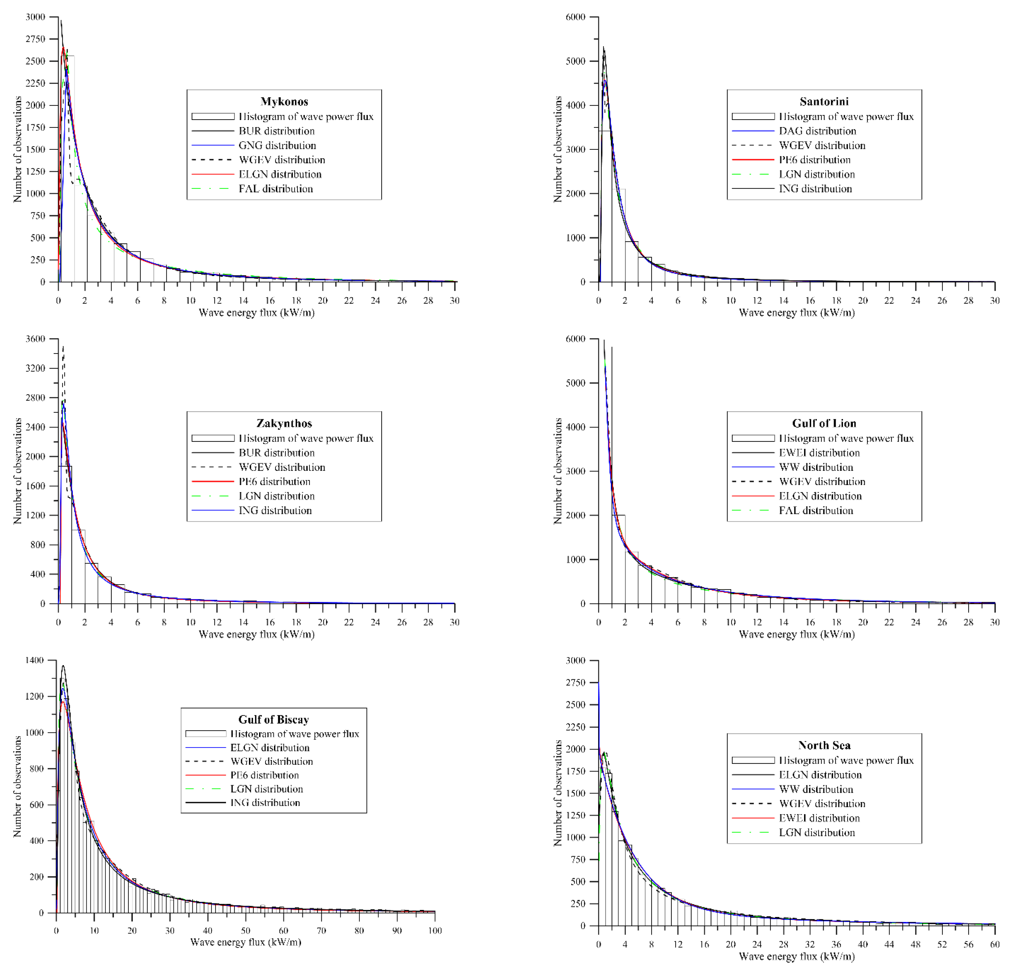
6.1. Univariate Distributions for Wave Energy Flux

BUR, DAG, ELGN, EW, FAL, GNG, LGN, LGL, PE6, WGEV, and WW distributions provide consistently good fit results with respect to the K-S and A-D tests at each examined location. At the next step of the evaluation, the above-mentioned distributions were evaluated by means of $R_{a,1}^2$. Based on the values of $R_{a,1}^2$, the following conclusions can be drawn:

(i)

The overall best fit is provided by ELGN distribution for North Sea (0.9998) and Gulf of Lion (0.9997); LGN distribution for Santorini (0.9995), Gulf of Biscay (0.9999), and Zakynthos (0.9989); and WGEV distribution for Mykonos (0.9987).

(ii)

The second-best fit is provided by LGN distribution for North Sea (0.9995), ING distribution for Santorini (0.9994), WGEV distribution for Zakynthos (0.9987), FAL distribution for Mykonos (0.9977), ELGN distribution for Gulf of Biscay (0.9998), and EW distribution for Gulf of Lion (0.9992).

(iii)

The third best fit is provided by WGEV distribution for North Sea (0.9993), Gulf of Biscay (0.9995), and Gulf of Lion (0.9992); PE6 distribution for Santorini (0.9992); ING distribution for Zakynthos (0.9981); and GNG distribution for Mykonos (0.9964).

In summary, the following univariate conventional distributions are further assessed in the bivariate case (as marginal cdfs for $P$):

(i)

For Mykonos: BUR, ELGN, FAL, GNG, and WGEV distributions;

(ii)

For Santorini: DAG, ING, LGN, PE6, and WGEV distributions;

(iii)

For Zakynthos: BUR, ING, LGN, PE6, and WGEV distributions;

(iv)

For Gulf of Lion: EW, ELGN, FAL, WGEV, and WW distributions;

(v)

For Gulf of Biscay: ELGN, ING, LGN, PE6, and WGEV distributions;

(vi)

For North Sea: ELGN, EW, LGN, WGEV, and WW distributions.

The parameters for each candidate conventional distribution, along with the corresponding parameters and the weighting parameter $\omega$ of the two mixture distributions, are presented in

Table 5. Parameters of the five best-fit univariate conventional and mixture distributions for the examined locations.

Locations	Probability Distributions and Parameters
Mykonos	BUR	ELGN	FAL	GNG	WGEV
	2.162, 0.975, 5.470, 0.099	8.388, 0.535, 1.253, 0.164	1.687, 1.879, 0.070	0.295, 5.866, 0.006, 0.098	2.541, 0.500, 0.657, 2.107, 2.366, 0.248
Santorini	DAG	ING	LGN	PE6	WGEV
	1.296, 1.284, 0.917, 0.124	1.079, 2.798, 0.054	1.246, 0.222, 0.121	1.837, 1.560, 0.998, 0.123	4.741, 0.330, 0.776, 0.926, 1.064, 0.072
Zakynthos	BUR	ING	LGN	PE6	WGEV
	1.442, 1.069, 2.259, 0.133	1.131, 3.720, 0.000	1.435, 0.317, 0.129	1.215, 1.485, 1.823, 0.133	3.317, 0.401, 0.797, 1.363, 1.455, 0.173
Gulf of Lion	EW	ELGN	FAL	WGEV	WW
	0.531, 0.770, 5.213, 0.280	0.533, 1.556, 0.991, 0.446	2.046, 1.474, −0.027	1.034, 0.653, 0.501, 3.256, 4.122, 0.510	0.752, 4.773, 1.238, 0.412, 0.779
Gulf of Biscay	ELGN	ING	LGN	PE6	WGEV
	67.660, 2.001, 1.215, 0.098	6.641, 21.057, −0.405	1.363, 2.122, 0.151	1.456, 1.462, 8.341, 0.171	1.672, 3.171, 0.681, 9.622, 11.027, 0.321
North Sea	ELGN	EW	LGN	WGEV	WW
	1.026, 1.890, 1.347, 0.073	5.397, 0.854, 25.724, 0.599	1.428, 1.744, −0.050	0.797, 15.952, 0.896, 2.506, 2.298, 0.529	1.029, 5.205, 0.842, 24.339, 0.568

. The presented parameters are the following:

(1)

Conventional distributions: For DAG, BUR, and GNG: $k,a, b,g$; FAL and LGL: $a, b,g$; LGN: $s, m,g$; PE6: $a_1,a_2, b,g$; GEV: $\xi ,\sigma , \mu ,$; ING: $l, m,g$; WEI: $a, b$;

(2)

Mixture distributions: WGEV: $a, b,\xi ,\sigma , \mu ,\omega$; WW: ${\alpha }_1,b_1,{\alpha }_2,b_2, \omega$; ELGN: $\mu ,s, m, \omega$; EW: $\mu ,a,b, \omega$.

In Figure 3, the best-fit distributions along with the corresponding histograms for wave power flux at the examined locations are presented. The range of the values on the $x$—axis varies, depending on the corresponding behaviour at each examined location, while the bin size of the histograms was kept the same, i.e., 1 kW/m.

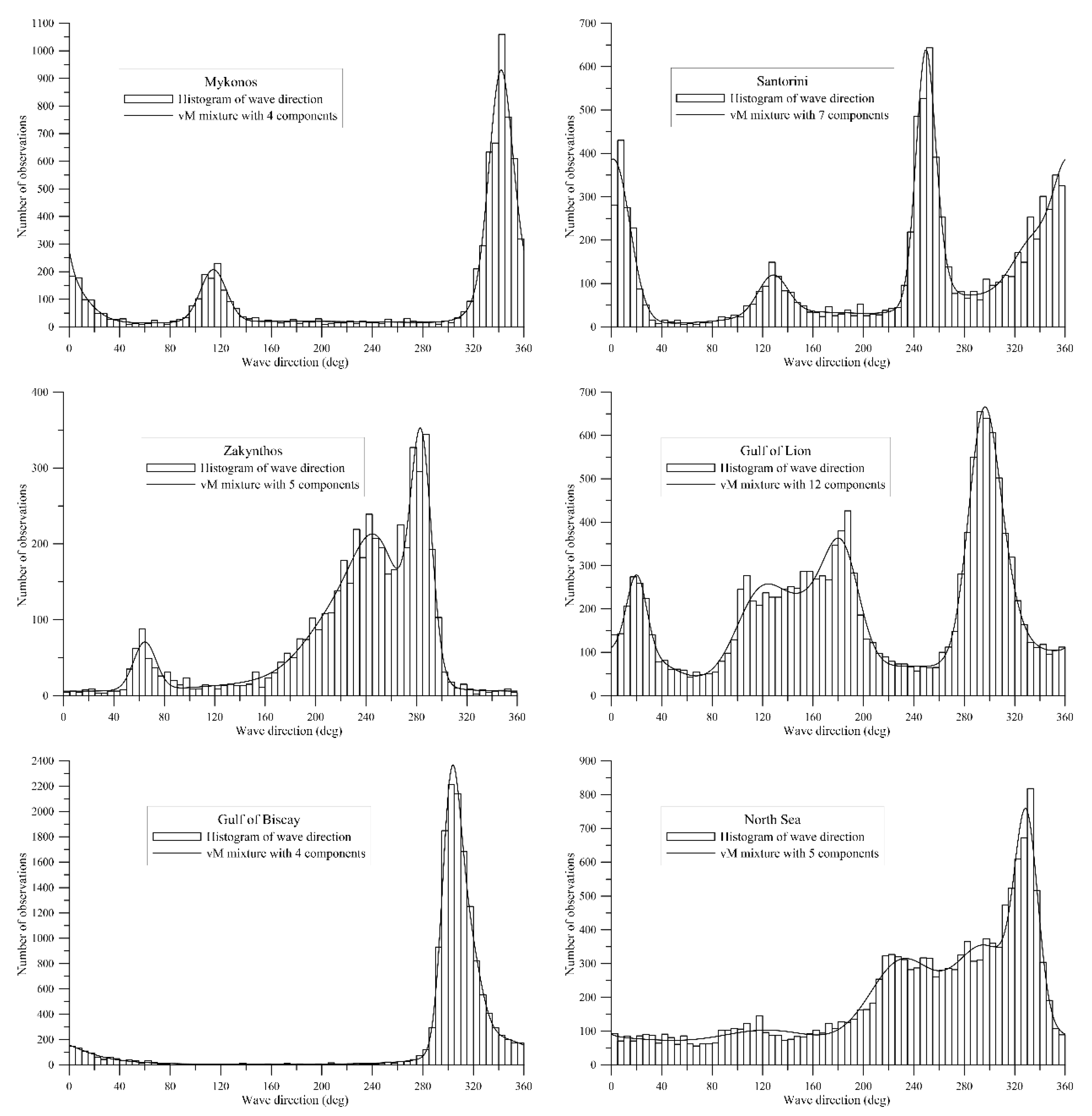
6.2. Univariate Distributions for Mean Wave Direction

In

Table 6. Parameters of the best-fit vM mixtures $\left(\kappa ,\mu ,\omega \right)$ for the examined locations.

	Locations
Parameters, $\mathit{i}=1,2,\cdots$	Mykonos	Santorini	Zakynthos	Gulf of Lion	Gulf of Biscay	North Sea
${\kappa }_i$	9.07, 0.22, 39.79, 31.42	61.22, 33.96, 10.38, 1.13, 2.58, 22.99, 23.52	41.69, 8.73, 48.06, 4.78, 0.57	52.47, 16.17, 1.91, 25.29, 7.87, 16.01, 6.54, 2.26, 3.53, 6.13, 17.38, 3.16	33.18, 61.92, 1.27, 4.62	4.70, 1.22, 5.40, 39.32, 1.60
${\mu }_i$	−0.17, −3.10, −0.32, 1.99	−1.94, −1.88, −0.41, 2.79, −1.34, 0.07, 2.24	1.12, −1.92, −1.33, −2.49, −2.99	0.35, −1.00, −1.34, −1.15, 2.06, −1.03, 2.82, −0.27, −2.30, −0.92, −3.08, 0.39	−0.79, −1.01, −0.41, −0.41	−2.26, 0.07, −1.11, −0.53, 2.21
${\omega }_i$	0.25, 0.16, 0.46, 0.13	0.19, 0.09, 0.18, 0.12, 0.14, 0.22, 0.06	0.06, 0.31, 0.25, 0.22, 0.16	0.05, 0.06, 0.05, 0.14, 0.16, 0.06, 0.14, 0.06, 0.05, 0.04, 0.11, 0.08	0.28, 0.46, 0.10, 0.15	0.26, 0.13, 0.26, 0.18, 0.16

, the parameters of the mixtures of vM distributions for $\Theta$ modelling are summarized. In terms of BIC, wave direction at Athos, Zakynthos, and North Sea is best described with five components of the vM mixtures, at Mykonos with four, at Santorini with seven, and at the Gulf of Lion with twelve.

In Figure 4, the histograms of mean wave direction for the examined locations are shown along with the plotted lines for vM mixtures.

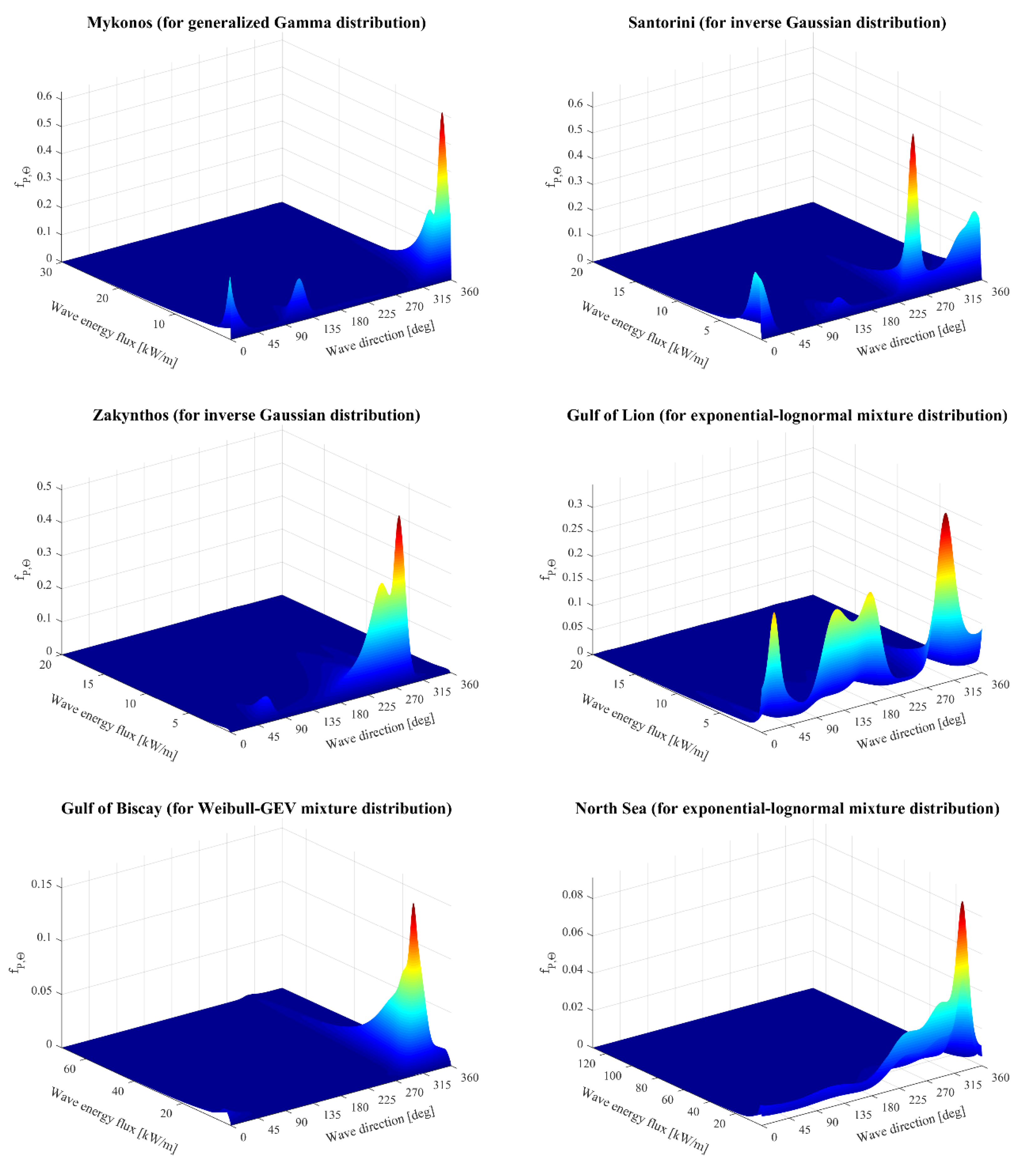
6.3. Joint Pdf for Wave Energy Flux and Direction

The parameters of the vM mixture $\left(\kappa ,\mu ,\omega \right)$ for modelling $f_{{\Psi }_{P\Theta }}$ are also estimated (not provided here) for the examined locations and pdfs of wave energy flux. Since $f_{{\Psi }_{P\Theta }}$ is a smooth function, two components of the vM mixture are adequate for its description.

In

Table 7. Values of the $GC \left(\times {10}^6\right)$ goodness-of-fit criterion for the Johnson–Wehrly bivariate distribution for the examined locations along with the best fit distributions for wave energy flux. Boldface digits indicate the optimum value of $GC$.

Distributions	Locations
	Mykonos	Santorini	Zakynthos	Gulf of Lion	Gulf of Biscay	North Sea
BUR	1291		9328
DAG		781
ELGN	1085			347	2629	4058
EW				329		3780
FAL	1191			299
GNG	1376
ING		865	10,194
LGN		814	5337		2249	3717
PE6		793	6861		2633
WGEV	1144	689	8253	335	2743	3742
WW				325	2430	3806

, the values of the goodness-of-fit criteria for the bivariate parametric distributions are provided for the examined locations and datasets. Boldface numbers denote the best value obtained from all the examined bivariate families.

For Mykonos, the JW model with the GNG marginal distribution for wave flux, provides the optimum values for the $FC$ criterion. Let it be noted that for Mykonos, the optimal marginal distribution according to $R_{a,1}^2$, was WGEV mixture, while the GNG distribution provided the third best fit. For Santorini and Zakynthos, the ING distribution provides the optimum values for the $FC$ criterion, although the optimal marginal distribution was LGN distribution. It is reminded that the ING distribution provided the second-best fit for Santorini and the third best fit for Zakynthos in the univariate case.

For Gulf of Lion and North Sea, the JW model with the ELGN marginal distribution (for wave flux) provides the optimum $FC$ value. The same distribution provided the best fit for the univariate case for both locations. Finally, for Gulf of Biscay, the JW model with the WGEV mixture marginal distribution provides the optimum values for the $FC$ criterion. Let it be noted that the optimal marginal distribution according to $R_{a,1}^2$ was LGN distribution while the WGEV mixture distribution provided the third best fit for wave energy flux.

Regarding the involvement of the univariate distributions per se in the bivariate models, mixture distributions (ELGN and WGEV) for wave energy flux provide the best bivariate fits for the locations where numerical wave model data are available. For Santorini and Zakynthos, ING distribution provides the best bivariate fits while for Mykonos GNG provide the best bivariate fit. It can also be deduced that the best univariate conventional distribution (in terms of $R_{a,1}^2$) for wave energy flux does not necessarily provides the best fit in the bivariate case.

In Figure 5, the best bivariate model for modelling the variables of interest is plotted for each location.

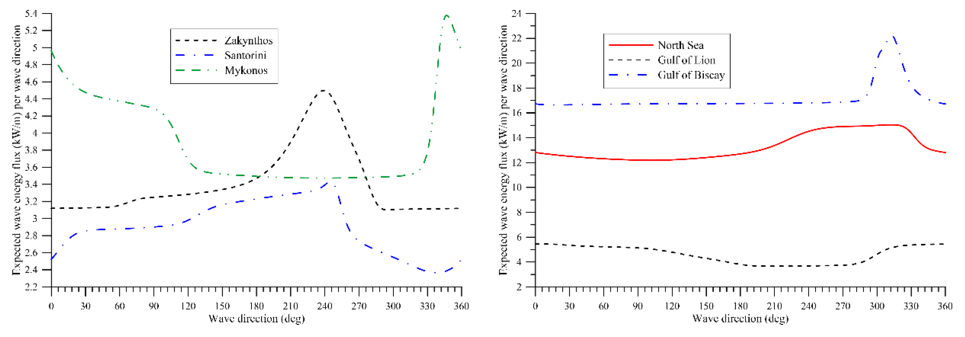
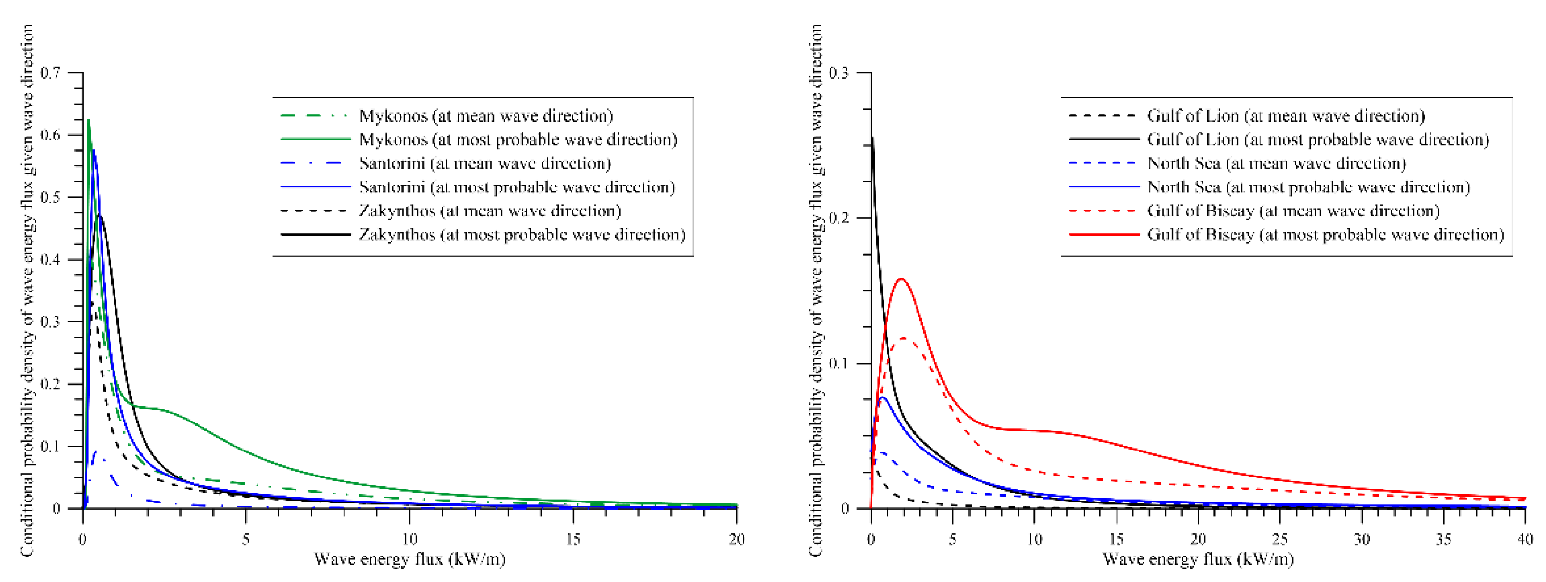
7. Application-Oriented Results

The preliminary assessment of the available wave energy in an area requires the estimation of the wave energy flux per sea state that is a function of significant wave height $H_S$ and energy period $T_e$ (see Equation (3)). Due to the temporal and spatial variability of $H_S$, $T_e$, wave direction $\Theta$, and sea water density $\rho$, more detailed information as regards wave flux for different occurrences of these variables at the specific area is required during the stage of wave farm design and layout. In this respect, for the evaluation of different aspects of the wave energy flux at a particular location, the wave energy flux–wave direction distribution should be used.

For a series of sea states $H_{S,i}, T_{e,i}, {\Theta }_i, i=1,2,\cdots ,n$, in an area, and for constant seawater density, the corresponding realizations $P_i,{\Theta }_i$ of the bivariate random variable $\left(P, \Theta \right)$ can be easily obtained, and its corresponding pdf $f_{P,\Theta }\left(p,\theta \right)$ can be estimated following the procedure described in Section 4. The mean wave energy flux for all wave directions can be obtained as follows:

$$E\left[P\right]={\int }_{P_{min}}^{P_{max}}{\int }_0^{2\pi }p{f}_{P,\Theta }\left(p,\theta \right)dpd\theta ,$$

(9)

where $P_{min}, P_{max}$ are the minimum and maximum values of $P$ observed in the area, respectively (or, equivalently, of $0.49H_S^2{T}_e$). From Equation (9), useful and detailed characteristics of the available directional wave energy flux in an area can be obtained. These characteristics can be further used as design parameters for the WEC and the wave farm layout.

For example, the conditional mean value of $P$ with respect to $\Theta$ can be derived as follows:

$$E\left[P|\Theta =\theta \right]={\int }_{P_{min}}^{P_{max}}p{f}_{P|\Theta }\left(p|\theta \right)dp,$$

(10)

where $f_{P|\Theta }\left(p|\theta \right)$ is the conditional pdf that is defined as follows:

$$f_{P|\Theta }\left(p|\theta \right)=\frac{f_{P,\Theta }\left(p,\theta \right)}{f_{\Theta }\left(\theta \right)}.$$

(11)

From the above relations, the wave energy flux per wave direction for various ranges of values of $H_S^2 T_e$, the wave energy flux per $0.49H_S^2{T}_e$ for various values of $\Theta$, and the distribution of wave energy flux for some critical directions of interest can also be obtained.

In Figure 6, the expected values of wave energy flux are depicted for the entire range of wave directions in the examined areas. As shown in Figure 6, for Zakynthos, Mykonos, and Gulf of Biscay, the highest values of the expected values of wave energy flux are concentrated in relatively narrow bands of wave direction. For Santorini, North Sea, and Gulf of Lion, the wave direction sectors that provide large values for the expected wave energy flux are rather wide.

In Figure 7, the distribution of wave energy flux for particular directions of interest, i.e., the mean and the most probable direction (based on the histograms of Figure 4) are depicted for the examined locations. It is observed that wave energy flux has the highest likelihood for the most probable wave direction at all examined locations. Let it be noted that regarding the examined locations with measured data, Mykonos is the only one where the likelihood remains high enough for values of wave energy flux above 5 kW/m, denoting that this area can be candidate for a more detailed assessment of wave energy resource. Moreover, it is clear that the Gulf of Biscay is characterized by a very energetic wave climate (especially for the most probable wave direction), which renders this location very promising for wave energy utilization.

8. Conclusions

The joint modelling of wave energy flux and wave direction in an area is important for wave energy projects. For instance, wave resource assessment issues and, in turn, WEC siting problems can be mitigated by constructing the most appropriate bivariate model based on real world data, attaining in this way economic viability of the corresponding projects. In this work, the Johnson–Wehrly parametric model was examined for the joint probabilistic description of wave energy flux and wave direction, after evaluating various conventional distributions for the linear variable. The proposed parametric bivariate models were constructed by considering the corresponding marginal distributions along with an appropriate dependence structure of the involved variables. The performance of the bivariate models was evaluated based on a global goodness-of-fit criterion, formed as a combination of RMSE, MAE, IA, ${\chi }^2$, and $R_{a,2}^2$. The models were applied for six long-term wave energy flux and wave direction time series, which were obtained from in situ measurements in the Greek Seas and wave model results in the western Mediterranean Sea, Gulf of Biscay, and the North Sea.

From the results, it was found that as regards wave energy flux, wave measurements were best modelled by the Inverse Gaussian and Generalized Gamma distributions while Exponential–Lognormal and Weibull–GEV mixture distributions provided overall the best fits for the examined locations where numerical model results were available. However, the above distributions were not the optimum ones in the evaluation of the univariate case, highlighting thus the necessity to evaluate a wide range of models for wave energy applications. The best bivariate model was also applied for the estimation of wave energy flux per wave direction as a real-world scenario in wave farm design for the examined locations.

This research revealed that an important prerequisite related to WEC developers is the provision of the corresponding power matrices for different mean wave directions. In this way, uncertainties as regards the annual wave energy production would be reduced while the optimization and the siting of a wave farm can be greatly facilitated.

References

1. Soukissian, T.H.; Denaxa, D.; Karathanasi, F.; Prospathopoulos, A.; Sarantakos, K.; Iona, A.; Georgantas, K.; Mavrakos, S. Marine Renewable Energy in the Mediterranean Sea: Status and Perspectives. Energies 2017, 10, 1512. [Google Scholar] [CrossRef] [Green Version]
2. Garcia, P.Q.; Sanabria, J.G.; Ruiz, J.A.C. The role of maritime spatial planning on the advance of blue energy in the European Union. Mar. Policy 2019, 99, 123–131. [Google Scholar] [CrossRef]
3. Besio, G.; Mentaschi, L.; Mazzino, A. Wave energy resource assessment in the Mediterranean Sea on the basis of a 35-year hindcast. Energy 2016, 94, 50–63. [Google Scholar] [CrossRef]
4. Arena, F.; LaFace, V.; Malara, G.; Romolo, A.; Viviano, A.; Fiamma, V.; Sannino, G.; Carillo, A. Wave climate analysis for the design of wave energy harvesters in the Mediterranean Sea. Renew. Energy 2015, 77, 125–141. [Google Scholar] [CrossRef]
5. Lavidas, G. Selection index for Wave Energy Deployments (SIWED): A near-deterministic index for wave energy converters. Energy 2020, 196, 117131. [Google Scholar] [CrossRef]
6. Guillou, N.; Chapalain, G. Annual and seasonal variabilities in the performances of wave energy converters. Energy 2018, 165, 812–823. [Google Scholar] [CrossRef] [Green Version]
7. Fairley, I.; Smith, H.C.M.; Robertson, B.; Abusara, M.; Masters, I. Spatio-temporal variation in wave power and implications for electricity supply. Renew. Energy 2017, 114, 154–165. [Google Scholar] [CrossRef] [Green Version]
8. Hiles, C.E.; Beatty, S.J.; De Andres, A. Wave energy converter annual energy production uncertainty using simulations. J. Mar. Sci. Eng. 2016, 4, 53. [Google Scholar] [CrossRef] [Green Version]
9. Stopa, J.E.; Filipot, J.-F.; Li, N.; Cheung, K.F.; Chen, Y.-L.; Vega, L. Wave energy resources along the Hawaiian Island chain. Renew. Energy 2013, 55, 305–321. [Google Scholar] [CrossRef]
10. Allahdadi, M.N.; He, R.; Neary, V.S. Predicting ocean waves along the US east coast during energetic winter storms: Sensitivity to whitecapping parameterizations. Ocean Sci. 2019, 15, 691–715. [Google Scholar] [CrossRef] [Green Version]
11. O’Connell, R.; de Montera, L.; Peters, J.L.; Horion, S. An updated assessment of Ireland’s wave energy resource using satellite data assimilation and a revised wave period ratio. Renew. Energy 2020, 160, 1431–1444. [Google Scholar] [CrossRef]
12. Ahn, S.; Haas, K.A.; Neary, V.S. Wave energy resource characterization and assessment for coastal waters of the United States. Appl. Energy 2020, 267, 114922. [Google Scholar] [CrossRef]
13. Wan, Y.; Zhang, J.; Meng, J.; Wang, J.; Dai, Y. Study on wave energy resource assessing method based on altimeter data—A case study in Northwest Pacific. Acta Oceanol. Sin. 2016, 35, 117–129. [Google Scholar] [CrossRef]
14. Sánchez, A.S.; Rodrigues, D.A.; Fontes, R.M.; Martins, M.F.; Kalid, R.D.A.; Torres, E.A. Wave resource characterization through in-situ measurement followed by artificial neural networks’ modeling. Renew. Energy 2018, 115, 1055–1066. [Google Scholar] [CrossRef]
15. Hanson, J.L.; Jensen, R.E. Wave system diagnostics for numerical wave models. In Proceedings of the 8th International Workshop on Wave Hindcasting and Forecasting, Oahu, HI, USA, 14–19 November 2004; pp. 231–238. [Google Scholar]
16. Allahdadi, M.N.; Gunawan, B.; Lai, J.; He, R.; Neary, V.S. Development and validation of a regional-scale high-resolution unstructured model for wave energy resource characterization along the US East Coast. Renew. Energy 2019, 136, 500–511. [Google Scholar] [CrossRef]
17. Christakos, K.; Varlas, G.; Cheliotis, I.; Spyrou, C.; Aarnes, O.J.; Furevik, B.R. Characterization of wind-sea- and swell-induced wave energy along the Norwegian coast. Atmosphere 2020, 11, 166. [Google Scholar] [CrossRef] [Green Version]
18. Guillou, N. Estimating wave energy flux from significant wave height and peak period. Renew. Energy 2020, 155, 1383–1393. [Google Scholar] [CrossRef]
19. Liberti, L.; Carillo, A.; Sannino, G. Wave energy resource assessment in the Mediterranean, the Italian perspective. Renew. Energy 2013, 50, 938–949. [Google Scholar] [CrossRef]
20. Neary, V.S.; Ahn, S.; Seng, B.E.; Allahdadi, M.N.; Wang, T.; Yang, Z.; He, R. Characterization of extreme wave conditions for wave energy converter design and project risk assessment. J. Mar. Sci. Eng. 2020, 8, 289. [Google Scholar] [CrossRef] [Green Version]
21. Allahdadi, M.N.C.; Allahyar, N.; McGee, M.R.L. Wave spectral patterns during a historical cyclone: A numerical model for cyclone gonu in the Northern Oman Sea. Open J. Fluid Dynam. 2017, 7, 131–151. [Google Scholar] [CrossRef] [Green Version]
22. Cuttler, M.V.; Hansen, J.E.; Lowe, R.J. Seasonal and interannual variability of the wave climate at a wave energy hotspot off the southwestern coast of Australia. Renew. Energy 2020, 146, 2337–2350. [Google Scholar] [CrossRef]
23. Wu, W.-C.; Wang, T.; Yang, Z.; García-Medina, G. Development and validation of a high-resolution regional wave hindcast model for U.S. West Coast wave resource characterization. Renew. Energy 2020, 152, 736–753. [Google Scholar] [CrossRef]
24. Ulazia, A.; Penalba, M.; Ibarra-Berastegui, G.; Ringwood, J.; Saénz, J. Wave energy trends over the Bay of Biscay and the consequences for wave energy converters. Energy 2017, 141, 624–634. [Google Scholar] [CrossRef]
25. Silverman, B.W. Density Estimation for Statistics and Data Analysis; Taylor & Francis: London, UK, 1986. [Google Scholar]
26. Scott, D.W. Multivariate Density Estimation: Theory, Practice, and Visualization; Wiley: New York, NY, USA, 1992. [Google Scholar]
27. Vanem, E. Joint statistical models for significant wave height and wave period in a changing climate. Mar. Struct. 2016, 49, 180–205. [Google Scholar] [CrossRef]
28. Bitner-Gregersen, E.M. Joint met-ocean description for design and operations of marine structures. Appl. Ocean Res. 2015, 51, 279–292. [Google Scholar] [CrossRef]
29. Li, W.; Isberg, J.; Chen, W.; Engström, J.; Waters, R.; Svensson, O. Bivariate joint distribution modeling of wave climate data using a copula method. Int. J. Energy Statist. 2016, 4, 1650015. [Google Scholar] [CrossRef]
30. Athanassoulis, G.; Belibassakis, K. Probabilistic description of metocean parameters by means of kernel density models 1. Theoretical background and first results. Appl. Ocean Res. 2002, 24, 1–20. [Google Scholar] [CrossRef]
31. Ferreira, J.; Soares, C.G. Modelling bivariate distributions of significant wave height and mean wave period. Appl. Ocean Res. 2002, 24, 31–45. [Google Scholar] [CrossRef]
32. Lucas, C.; Soares, C.G. Bivariate distributions of significant wave height and mean wave period of combined sea states. Ocean Eng. 2015, 106, 341–353. [Google Scholar] [CrossRef]
33. Myrhaug, D.; Leira, B.J.; Holm, H. Wave power statistics for individual waves. Appl. Ocean Res. 2009, 31, 246–250. [Google Scholar] [CrossRef]
34. Myrhaug, D.; Leira, B.J.; Holm, H. Wave power statistics for sea states. J. Offshore Mech. Arct. Eng. 2011, 133, 044501. [Google Scholar] [CrossRef]
35. López, I.; Andreu, J.; Ceballos, S.; Martínez de Alegría, I.; Kortabarria, I. Review of wave energy technologies and the necessary power-equipment. Renew. Sustain. Energy Rev. 2013, 27, 413–434. [Google Scholar] [CrossRef]
36. Pitt, E. Assessment of Performance of Wave Energy Conversion Systems; European Marine Energy Centre Ltd.: London, UK, 2009. [Google Scholar]
37. LaFace, V.; Arena, F.; Soares, C.G. Directional analysis of sea storms. Ocean Eng. 2015, 107, 45–53. [Google Scholar] [CrossRef]
38. Carballo, R.; E Sanchez, M.; Ramos, V.; Taveirapinto, F.; Iglesias, G. A high resolution geospatial database for wave energy exploitation. Energy 2014, 68, 572–583. [Google Scholar] [CrossRef] [Green Version]
39. Iglesias, G.; Carballo, R. Wave energy and nearshore hot spots: The case of the SE Bay of Biscay. Renew. Energy 2010, 35, 2490–2500. [Google Scholar] [CrossRef]
40. Soukissian, T.H. Probabilistic modeling of directional and linear characteristics of wind and sea states. Ocean Eng. 2014, 91, 91–110. [Google Scholar] [CrossRef]
41. Smith, H.C.M.; Fairley, I.; Robertson, B.; Abusara, M.; Masters, I. Wave resource variability: Impacts on wave power supply over regional to international scales. Energy Procedia 2017, 125, 240–249. [Google Scholar] [CrossRef] [Green Version]
42. Amrutha, M.M.; Kumar, V.S. Spatial and temporal variations of wave energy in the nearshore waters of the central west coast of India. Ann. Geophys. 2016, 34, 1197–1208. [Google Scholar] [CrossRef] [Green Version]
43. Wei, K.; Arwade, S.R.; Myers, A.T.; Valamanesh, V.; Pang, W. Effect of wind and wave directionality on the structural performance of non-operational offshore wind turbines supported by jackets during hurricanes. Wind. Energy 2016, 20, 289–303. [Google Scholar] [CrossRef]
44. Barj, L.; Stewart, S.; Stewart, G.; Lackner, M.; Jonkman, J.; Robertson, A. Wind/Wave Misalignment in the Loads Analysis of a Floating Offshore Wind Turbine; National Renewable Energy Lab (NREL): Golden, CO, USA, 2014. [Google Scholar]
45. Bachynski, E.E.; Kvittem, M.I.; Luan, C.; Moan, T. Wind-wave misalignment effects on floating wind turbines: Motions and tower load effects. J. Offshore Mech. Arct. Eng. 2014, 136, 041902. [Google Scholar] [CrossRef]
46. Lisboa, R.C.; Teixeira, P.R.; Fortes, C.J. Numerical evaluation of wave energy potential in the south of Brazil. Energy 2017, 121, 176–184. [Google Scholar] [CrossRef]
47. Soukissian, T.H.; Karathanasi, F.E. On the selection of bivariate parametric models for wind data. Appl. Energy 2017, 188, 280–304. [Google Scholar] [CrossRef]
48. Vega, J.L.; Rodríguez, G. Modelling mean wave direction distribution with the Von Mises model. WIT Trans. Ecol Environ. 2009, 126, 3–14. [Google Scholar]
49. Tofallis, C. Selecting the best statistical distribution using multiple criteria. Comput. Ind. Eng. 2008, 54, 690–694. [Google Scholar] [CrossRef] [Green Version]
50. Erdem, E.; Shi, J. Comparison of bivariate distribution construction approaches for analysing wind speed and direction data. Wind. Energy 2011, 14, 27–41. [Google Scholar] [CrossRef]
51. Soukissian, T.; Chronis, G. Poseidon: A marine environmental monitoring, forecasting and information system for the Greek seas. Mediterr. Mar. Sci. 2000, 1, 71. [Google Scholar] [CrossRef]
52. Soukissian, T.H.; Chronis, G.T.; Nittis, K.; Diamanti, C. Advancement of operational oceanography in Greece: The case of the Poseidon system. J. Atmospheric Ocean Sci. 2002, 8, 93–107. [Google Scholar] [CrossRef]
53. Korres, G.; Ravdas, M.; Zacharioudaki, A. Mediterranean Sea Waves Hindcast (CMEMS MED-Waves 2006–2017) (Version 1) [Data Set]. Copernicus Monitoring Environment Marine Service (CMEMS). Available online: https://doi.org/10.25423/CMCC/MEDSEA_HINDCAST_WAV_006_0122019 (accessed on 15 December 2020).
54. Poli, P.; Hersbach, H.; Dee, D.P.; Berrisford, P.; Simmons, A.J.; Vitart, F.; Laloyaux, P.; Tan, D.G.H.; Peubey, C.; Thépaut, J.-N.; et al. ERA-20C: An atmospheric reanalysis of the twentieth century. J. Clim. 2016, 29, 4083–4097. [Google Scholar] [CrossRef]
55. Romolo, A.; Arena, F. On Adler space-time extremes during ocean storms. J. Geophys. Res. Oceans 2015, 120, 3022–3042. [Google Scholar] [CrossRef]
56. Romolo, A.; Malara, G.; Laface, V.; Arena, F. Space–time long-term statistics of ocean storms. Probabilist. Eng. Mech. 2016, 44, 150–162. [Google Scholar] [CrossRef]
57. Fedele, F.; Lugni, C.; Chawla, A. The sinking of the El Faro: Predicting real world rogue waves during Hurricane Joaquin. Sci. Rep. 2017, 7, 11188. [Google Scholar] [CrossRef]
58. Fisher, N.I. Statistical Analysis of Circular Data, 1st ed.; Cambridge University Press: Cambridge, UK, 1993. [Google Scholar]
59. Galanis, G.; Chu, P.C.; Kallos, G.; Kuo, Y.-H.; Dodson, C.T.J. Wave height characteristics in the north Atlantic ocean: A new approach based on statistical and geometrical techniques. Stoch. Environ. Res. Risk Assess. 2011, 26, 83–103. [Google Scholar] [CrossRef] [Green Version]
60. Teixeira, R.; Nogal, M.; O’Connor, A. On the suitability of the generalized Pareto to model extreme waves. J. Hydraul. Res. 2018, 56, 755–770. [Google Scholar] [CrossRef] [Green Version]
61. Masseran, N.; Razali, A.M.; Ibrahim, K.; Latif, M.T. Fitting a mixture of von Mises distributions in order to model data on wind direction in Peninsular Malaysia. Energy Convers. Manag. 2013, 72, 94–102. [Google Scholar] [CrossRef]
62. Directional: A Collection of R Functions for Directional Data Analysis. Available online: https://cran.r-project.org/web/packages/Directional (accessed on 16 December 2020).
63. movMF: Mixtures of von Mises-Fisher Distributions. Available online: https://cran.r-project.org/web/packages/movMF (accessed on 18 December 2020).
64. Dong, S.; Wang, N.; Lu, H.; Tang, L. Bivariate distributions of group height and length for ocean waves using Copula methods. Coast. Eng. 2015, 96, 49–61. [Google Scholar] [CrossRef]
65. Antão, E.; Soares, C.G. Approximation of bivariate probability density of individual wave steepness and height with copulas. Coast. Eng. 2014, 89, 45–52. [Google Scholar] [CrossRef]
66. Qu, X.; Shi, J. Bivariate modeling of wind speed and air density distribution for long-term wind energy estimation. Int. J. Green Energy 2010, 7, 21–37. [Google Scholar] [CrossRef]
67. Athanassoulis, G.A.; Skarsoulis, E.K.; Belibassakis, K.A. Bivariate distributions with given maringals with an application to wave climate description. Appl. Ocean Res. 1994, 16, 1–17. [Google Scholar] [CrossRef]
68. Johnson, R.A.; Wehrly, T.E. Some angular-linear distributions and related regression models. J. Am. Stat. Assoc. 1978, 73, 602. [Google Scholar] [CrossRef]
69. Zhou, J.; Erdem, E.; Li, G.; Shi, J. Comprehensive evaluation of wind speed distribution models: A case study for North Dakota sites. Energy Convers. Manag. 2010, 51, 1449–1458. [Google Scholar] [CrossRef]
70. Kollu, R.; Rayapudi, S.R.; Narasimham, S.; Pakkurthi, K.M. Mixture probability distribution functions to model wind speed distributions. Int. J. Energy Environ. Eng. 2012, 3, 27. [Google Scholar] [CrossRef] [Green Version]
71. Soukissian, T. Use of multi-parameter distributions for offshore wind speed modeling: The Johnson S-B distribution. Appl. Energy 2013, 111, 982–1000. [Google Scholar] [CrossRef]
72. Ouarda, T.; Charron, C.; Shin, J.-Y.; Marpu, P.; Al-Mandoos, A.; Al-Tamimi, M.; Ghedira, H.; Al Hosary, T. Probability distributions of wind speed in the UAE. Energy Convers. Manag. 2015, 93, 414–434. [Google Scholar] [CrossRef] [Green Version]
73. Ramanathan, R. Selecting the best statistical distribution—A comment and a suggestion on multi-criterion evaluation. Comput. Ind. Eng. 2005, 49, 625–628. [Google Scholar] [CrossRef]
74. Wang, Y.; Yam, R.C.; Zuo, M.J. A multi-criterion evaluation approach to selection of the best statistical distribution. Comput. Ind. Eng. 2004, 47, 165–180. [Google Scholar] [CrossRef]
Figure 1. Locations of buoys and model grid points used in the analysis.
Processes 09 00460 g001
Figure 2. Directional histograms of wave power flux (kW/m) for the examined locations.
Processes 09 00460 g002aProcesses 09 00460 g002b
Figure 3. Histograms of wave energy flux along with the best fits from the corresponding probability density function at the examined locations.
Processes 09 00460 g003
Figure 4. Histograms of wave direction along with the fitted vM mixture distributions for the examined locations.
Processes 09 00460 g004
Figure 5. Bivariate best-fit pdfs of wave energy flux and mean wave direction for the examined locations.
Processes 09 00460 g005
Figure 6. Expected value of wave energy flux as function of wave direction at the examined locations. Left panel: Mykonos, Santorini, and Zakynthos. Right panel: Gulfs of Lion and Biscay and North Sea.
Processes 09 00460 g006
Figure 7. Distribution of wave energy flux for the mean and the most probable wave direction at the examined locations. Left panel: Mykonos, Santorini, and Zakynthos. Right panel: Gulfs of Lion and Biscay and North Sea.
Processes 09 00460 g007