Distribution-Independent Empirical Modeling of Particle Size Distributions—Coarse-Shredding of Mixed Commercial Waste

Abstract

Particle size distributions (PSDs) belong to the most critical properties of particulate materials. They influence process behavior and product qualities. Standard methods for describing them are either too detailed for straightforward interpretation (i.e., lists of individual particles), hide too much information (summary values), or are distribution-dependent, limiting their applicability to distributions produced by a small number of processes. In this work the distribution-independent approach of modeling isometric log-ratio-transformed shares of an arbitrary number of discrete particle size classes is presented. It allows using standard empirical modeling techniques, and the mathematically proper calculation of confidence and prediction regions. The method is demonstrated on coarse-shredding of mixed commercial waste from Styria in Austria, resulting in a significant model for the influence of shredding parameters on produced particle sizes (with classes: >80 mm, 30–80 mm, 0–30 mm). It identifies the cutting tool geometry as significant, with a p-value < 10⁻⁵, while evaluating the gap width and shaft rotation speed as non-significant. In conclusion, the results question typically chosen operation parameters in practice, and the applied method has proven to be valuable addition to the mathematical toolbox of process engineers.

1. Introduction

The size distribution belongs to the most critical properties of solid particulate materials, and particularly mixed solid waste, for example: The quality classes of solid recovered fuels (SRF) demand specific maximum particle sizes [1]. The particle size distribution (PSD) of the organic fraction of municipal waste impacts its anaerobic digestion [2]. The particle sizes of municipal solid waste influence the yields of dry gas, char, and tar in fixed bed reactor pyrolysis [3]. And the PSD influences the mass throughput of robotic sorters, which are limited by picks per hour [4]; hence, smaller particle sizes (and the corresponding smaller weights) decrease the possible mass throughput.

Concerning mixed commercial waste, besides the PSD’s relevance as a technical quality criterion for processing products (e.g., SRF [5]), and its influence on the performance of reactors and processing machines (e.g., wind sifters [6]), different types of materials also concentrate in different particle size ranges (e.g., sorting analysis by Khodier et al. [7] and the size distribution of different plastic types according to Möllnitz et al. [8]). Hence, beyond influencing the shares of a plant’s throughput that pass specific machines (due to material flow separation by screens), the PSD also determines the kinds of materials that pass through these machines.

Therefore, beneficial PSDs increase the effectiveness, as well as economic and ecologic efficiency of mixed solid waste treatment. Consequently, the PSD of mixed solid waste is deliberately influenced during mechanical processing, which is usually the first treatment stage for this kind of material, mainly through a combination of shredding and sieving [1,2,3,7,9,10,11,12,13].

1.1. Describing Particle Size Distributions

Strictly speaking, the PSD of a collective is described as a list of the individual particles’ sizes. But the representation as such a list is not suitable for analyzing and comparing PSDs. Consequently, various more useful methods for describing PSDs exist, which were summarized by Polke et al. [14]: Collectives of particles are often described through average equivalent diameters. An example is the Sauter diameter $d_S$, which gives information on the specific surface of the collective (Equation (1), where $V_t$ is the total volume of all particles, and $A_t$ is the total surface area of all particles).

$$d_S=6V_t/A_t$$

(1)

Often, information on the width of the distribution is also essential. Consequently, measures of this width are frequently provided. Examples are the sample standard deviation $S$ (Equation (2), where $d_i$ is the size of the $i$^th particle, $\overline{d}$ is the arithmetic average size, and $N$ is the number of particles), or distribution-independent measures of the width, as shown, for example, in Equation (3) (where $W$ is the width, and $d_b$ is the $b$^th percentile particle size).

$$S=\sqrt{\frac{{\sum }_{i=1}^N{\left(d_i-\overline{d}\right)}^2}{N-1}}$$

(2)

$$W=\frac{d_{75}-d_{25}}{d_{50}}$$

(3)

Considering the described influence of the PSD on the path individual particles take through a plant, it is essential in mechanical waste processing to have more detailed knowledge on it than just summary values. Hence, the results of a PSD analysis are often reported graphically: the frequency density is shown in a histogram [15], where particle sizes are summarized into particle size classes (PSCs)—which is also the level of information obtained from sieve analyses (Figure 1a). Another representation, which is more suitable for comparing PSDs, is the sum distribution (Figure 1b) [14].

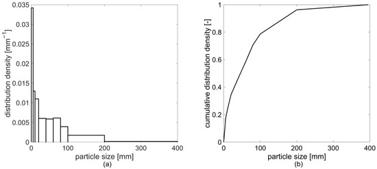
Figure 1. Representation of the overall particle size distribution (PSD) of a mixed commercial waste according to Reference [7]: (a) frequency density; (b) cumulative frequency density.

These graphical representations correspond to an empirical distribution [15]. As the sample size approaches infinity and the class width approaches zero, the histogram’s representation becomes a continuous function: the probability density function (PDF). This PDF can also be approximated from analyses, where only summary information on discrete PSCs is available (e.g., sieve analyses), for example, through cubic splines [16] or Kernel density estimation [17].

Sometimes, the PDF can be approximately described by an analytical expression. In such cases, reporting the momentums of such an analytical distribution is sufficient to describe the PSD. So, for example, reporting the arithmetic mean particle size $\overline{d}$ of the sample and its standard deviation $S$, usually implies the underlying assumption of a normal distribution, according to Equation (4), where $q\left(d\right)$ is the probability density or frequency density for particles of size $d$, $\mu$ is the arithmetic average of the population, which is estimated through $\overline{d}$, and $\sigma$ is the population’s standard deviation, which is estimated through $S$ [18].

$$q\left(d\right)=\frac{1}{\sqrt{2\pi {\sigma }^2}}·\exp \left(-\frac{{\left(d-\mu \right)}^2}{2{\sigma }^2}\right)$$

(4)

Three further analytical PDFs, are reported as being relevant to the description of PSDs [14]: The log-normal distribution describes materials, where the logarithm of the particle size follows a normal distribution. It is a positively skewed distribution, which—in contrast to the normal distribution—only includes positive and, therefore, meaningful particle sizes. It is shown in Equation (5), where $\mu$ and $\sigma$ are estimated by the arithmetic average and the sample standard deviation of the logarithm of the particle sizes.

$$q\left(d\right)=\{\begin{array}{ll}0\hfill & \mathrm{if} d<0\hfill \\ \frac{1}{d\sqrt{2\pi {\sigma }^2}}·\exp \left(-\frac{{\left(\log \left(d\right)-\mu \right)}^2}{2{\sigma }^2}\right)\hfill & \mathrm{otherwise}\hfill \end{array}$$

(5)

The Gates-Gaudin-Schuhmann (GGS) distribution [19] is an empirical approximation that is often suitable for describing products of coarse comminution processes. Its parameters are the maximum particle size $d_{max}$ and the uniformity parameter $m_u$. Its PDF is shown in Equation (6).

$$q\left(d\right)=\{\begin{array}{ll}0\hfill & \mathrm{if} d<0 \mathrm{or} d>d_{max}\hfill \\ \frac{m_u}{d_{max}}{\left(\frac{d}{d_{max}}\right)}^{m_u-1}\hfill & \mathrm{otherwise}\hfill \end{array}$$

(6)

The Rosin-Rammler-Sperling-Bennet (RRSB) distribution [20] is also an empirical approximation. Its first parameter $d^{\prime }$ is equal to the particle size, where the cumulative frequency density reaches the value $1-1/e\approx 0.632$, and its second parameter $n_u$ is a uniformity parameter. Its PDF is shown in Equation (7). The RRSB distribution is often used for describing products of fine comminution and dusts. Examples of the discussed distributions are shown in Figure 2.

$$q\left(d\right)=\{\begin{array}{ll}0\hfill & \mathrm{if} d<0\hfill \\ \frac{n_u}{d^{\prime }}{\left(\frac{d}{d^{\prime }}\right)}^{n_u-1}\exp \left[-{\left(\frac{d}{d^{\prime }}\right)}^{n_u}\right]\hfill & \mathrm{otherwise}\hfill \end{array}$$

(7)

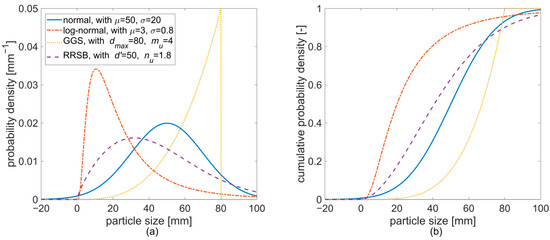
Figure 2. Frequency density (a) and cumulative frequency density (b) of a normal, log-normal, Gates-Gaudin-Schuhmann (GGS), and Rosin-Rammler-Sperling-Bennet (RRSB) distribution.

1.2. Modeling Particle Size Distributions

Products’ PSDs result from their original condition and the kinds and parameters of machines that process them. Hence, to beneficially influence PSDs through process design and the choice and parametrization of machines, modeling and predicting them is desirable.

The most sophisticated and advantageous models are physical models, which provide an in-depth understanding of the phenomena that influence PSDs. Simulations based on such models are usually implemented using the discrete element method (DEM). Examples in literature are the works of Sinnott and Cleary [21] on the particle flows and breakage in impact crushers, Lee et al. [22] on breakage and liberation behavior of recycled aggregates from impact-breakage of concrete waste, and Dong et al. [23] on particle flow and separation on vibrating screens.

While DEM-based models improve process understanding, they also require high amounts of computational resources and detailed models and data on the processing machines and the materials to be comminuted, which limits their applicability in practice in many cases [24]: no published models, for example, incorporate the variability of materials, geometries and particle interactions for real mixed solid waste.

When physical models cannot be used, empirical regression models can deliver basic insights on machine and parameter influences on PSDs. For ensuring the reliability of the results, it is essential to involve statistical analyses for finding and interpreting the models. For scalar target values, the procedure has been thoroughly described by Khodier et al. [24], based on the example of the parametrization-dependent energy demand and throughput behavior of coarse shredders for mixed commercial waste.

PSDs are non-scalar: they are either described as PDFs, which are continuous functions, or as compositions of PSCs and, therefore, as multivariate vectors. Analytical PDFs, as those presented in Section 1.1., are defined by a set of momentums, which can also be treated as multivariate vectors. Consequently, modeling PSDs requires extensions of the methods used by Khodier et al. [24] to multivariate dependent variables.

The most widely applied variation of regression modeling is linear regression. It relates one or more dependent variables to one or more independent variables based on a set of linear regression coefficients. Its most general form—which is relevant to this work—is multivariate multiple linear regression, which involves multiple independent variables and multivariate dependent variables. Its model Equation is shown in Equation (8) [25]. The matrix $\mathit{Y}$ (Equation (9)) is the $P\times R$ matrix of $P$ observations of the $R$-variate vector of the dependent variable, with elements $y_{p,r}$. $\mathit{\epsilon }$ (Equation (12)) is also a $P\times R$ matrix and shows the corresponding model residuals ${\epsilon }_{p,r}$. $\mathit{X}$ (Equation (10)) is a $P\times \left(Q+1\right)$ matrix of the settings $x_{p,q}$ of the $Q$ independent variables corresponding to the $P$ observations. Its first column (which is indexed with 0) is a column of ones, corresponding to constant terms in linear regressions. And the matrix $\mathit{\beta }$ (Equation (11)) contains the $\left(Q+1\right)\times R$ regression coefficients ${\beta }_{q,r}$.

$$\mathit{Y}=\mathit{X}·\mathit{\beta }+\mathit{\epsilon }$$

(8)

$$\mathit{Y}=\left[\begin{array}{cccc}{y}_{1,1}& y_{1,2}& \cdots & y_{1,R}\\ y_{2,1}& y_{2,2}& \cdots & y_{2,R}\\ ⋮& ⋮& \ddots & ⋮\\ y_{P,1}& y_{P,2}& \cdots & y_{P,R}\end{array}\right]$$

(9)

$$\mathit{X}=\left[\begin{array}{ccccc}{x}_{1,0}& x_{1,1}& x_{1,2}& \cdots & x_{1,Q}\\ x_{2,0}& x_{2,1}& x_{2,2}& \cdots & x_{2,Q}\\ ⋮& ⋮& ⋮& \ddots & ⋮\\ x_{P,0}& x_{P,1}& x_{P,2}& \cdots & x_{P,Q}\end{array}\right]=\left[\begin{array}{ccccc}1& x_{1,1}& x_{1,2}& \cdots & x_{1,Q}\\ 1& x_{2,1}& x_{2,2}& \cdots & x_{2,Q}\\ ⋮& ⋮& ⋮& \ddots & ⋮\\ 1& x_{P,1}& x_{P,2}& \cdots & x_{P,Q}\end{array}\right]$$

(10)

$$\mathit{\beta }=\left[\begin{array}{cccc}{\beta }_{0,1}& {\beta }_{0,2}& \cdots & {\beta }_{0,R}\\ {\beta }_{1,1}& {\beta }_{1,2}& \cdots & {\beta }_{1,R}\\ ⋮& ⋮& \ddots & ⋮\\ {\beta }_{Q,1}& {\beta }_{Q,2}& \cdots & {\beta }_{Q,R}\end{array}\right]$$

(11)

$$\mathit{\epsilon }=\left[\begin{array}{cccc}{\epsilon }_{1,1}& {\epsilon }_{1,2}& \cdots & {\epsilon }_{1,R}\\ {\epsilon }_{2,1}& {\epsilon }_{2,2}& \cdots & {\epsilon }_{2,R}\\ ⋮& ⋮& \ddots & ⋮\\ {\epsilon }_{P,1}& {\epsilon }_{P,2}& \cdots & {\epsilon }_{P,R}\end{array}\right]$$

(12)

The resulting model is obtained by minimizing the sum of squares of the residuals ${\epsilon }_{p,r}$. It is shown in Equation (13), where $\widehat{\mathit{Y}}$ is the matrix of the $P\times R$ model predictions ${\widehat{y}}_{p,r}$ for the dependent variable, corresponding to the observations in $\mathit{Y}$, and $\widehat{\mathit{\beta }}$ is the matrix of the $\left(Q+1\right)\times R$ least-squares estimates ${\widehat{\beta }}_{q,r}$ of the regression coefficients in $\mathit{\beta }$.

$$\widehat{\mathit{Y}}=\mathit{X}·\widehat{\mathit{\beta }}$$

(13)

For linear regression models, it is necessary to describe the dependent variable as a vector of a fixed length. In the case of analytical PDFs, this is the vector of the momentums. So, the immediate result of a model for these momentums is the vector of their expected values, and the corresponding confidence bands. From there, the PDF and its confidence region can be calculated.

Theoretically, $\widehat{\mathit{\beta }}$ can also be calculated from $Q$ univariate linear regressions. The resulting values ${\widehat{\beta }}_{q,r}$ are identical. But multivariate methods, involving multivariate linear regression and multivariate analysis of variance (MANOVA, e.g., Reference [26]), are preferable: they allow a more accurate calculation of confidence regions, considering correlations between the momentums. Moreover, the evaluation of parameter’s significance should be based on multivariate considerations to find coherent models for the resulting—interdependent—distribution of the particle sizes.

Analytical PDFs are practical, as they allow a detailed description of PSDs with a small number of variables—the momentums. However, only few processes produce PSDs that follow analytical functions, according to Polke et al. [14]. Consequently, methods for distribution-independent modeling of PSDs are also needed, which is especially true for the mechanical processing of mixed solid waste, considering the variety of processing machines used there: e.g., shredders, screens, magnetic separators, and sensor-based sorters [10].

Empirical distributions allow the distribution-independent description of PSDs: particle sizes are amalgamated to $D$ discrete PSCs. As a result, the PSD is described as a composition—a $D$-dimensional vector of the shares of those PSCs.

Mathematically, the compositional nature of the vector of PSCs has wide-reaching consequences: $D$-dimensional compositions are constrained to a vector space called the $D$-dimensional simplex ${\mathit{S}}^{\left(\mathit{D}\right)}$, which is a sub-space of the $D$-dimensional real space ${\mathit{R}}^{\left(\mathit{D}\right)}$ [27]. Compositions, being simplicial vectors, have specific common properties: Their $D$ parts are not linearly independent. This results from a summation constraint: their parts sum up to a fixed constant, e.g., 1 or 100%. Furthermore, parts may only have positive values or zero. So, more precisely, ${\mathit{S}}^{\left(\mathit{D}\right)}$ is a sub-space of ${\mathit{R}}_{\mathbf{0}}^{+\left(\mathit{D}\right)}$. The most well-known representation of a simplex is the ternary diagram (see, e.g., Reference [28]), which shows the three-dimensional simplex.

When modeling simplicial vectors, the constraints of the simplex and the interdependence of the compositional parts must be considered. While Khodier et al. [29] report the empirical observation that the constraints are automatically fulfilled for the prediction values $\widehat{\mathit{Y}}$, if all observations in $\mathit{Y}$ are valid compositions, this does not apply to corresponding confidence regions. Hence, different methods were developed in the past decades to handle and model simplicial data.

The most widely applied approach for handling compositions is transforming data using log-ratios, as suggested by Aitchison [30]. There are many kinds of such log-ratios, but the state of the art approach in the compositional data community is the application of so-called isometric log-ratios (ilr) (as proposed by Egozcue [31]), according to Reference [32]. These are bijective projections of the $D$-dimensional Simplex onto a $\left(D-1\right)$-dimensional real-space with an orthonormal basis [27]. The resulting ilr-coordinates are unconstrained, linearly independent coordinates. Hence, standard statistics can be applied in the projected log-ratio space, as demonstrated, for example, by Edjabou et al. [33] for waste composition analysis. Consequently, the use of ilr-transformations allows the application of standard multivariate multiple linear regression to predict PSDs, described as empirical distributions.

In this work, the approach of modeling influences on empirical PSDs using multivariate multiple linear regression and ilrs is applied on particle size data, using the programming language R. The data was obtained within Khodier et al.’s [24] industry-scale coarse-shredding experiments with real mixed commercial waste. Based on this example, this work aims at presenting the method to the process engineering and waste processing communities, enabling the distribution-independent empirical modeling of particle size distributions, while preserving all relevant information. Moreover, the method’s suitability for PSD modeling and its limitations and potential pitfalls in the interpretation of the results are discussed. And, finally, insights on the influences of coarse shredders’ parameters on the PSDs of mixed commercial waste are presented, complementing findings of Khodier et al. [24] on their effects on shredders’ throughput behavior and energy demand.

2. Materials and Methods

2.1. Experimental Design and Setup

The choice of the experimental design and the shredding experiment setup have been explained in detail by Khodier et al. [24]. Hence, they are only summarized in the following. The extension of the experiment with material sampling and particle size analysis are described in detail.

2.1.1. Experimental Design

The shredding experiment examines the influence of three independent variables on the throughput behavior and energy demand of a Terminator 5000 SD, which is a single-shaft shredder from the Austrian company Komptech GmbH (Frohnleiten, Austria)—a research partner in the funded project ReWaste 4.0. These independent variables are the radial gap width $w$, the shaft rotation speed $s$, and the cutting tool geometry $c$. The factor range of $w$ was defined from 0% to 100% of the maximum gap width, with discrete levels at a step size of 10%. The minimum of the factor range of $s$ was chosen at 60% and the maximum at 100% of the maximum shaft rotation speed of 31 rpm, again width discrete 10% steps. Concerning $c$, three different geometries are examined, called “F”, “XXF”, and “V” (for more details, cf. Reference [24] and Figure A1 and Table A1 in the Appendix A).

The factors are coded for the design and analysis of the experiment: for the numerical factors $s$ and $w$, their range is adjusted to −1 to 1, representing the minimum and maximum factor settings. Concerning the nominal factor $c$, it is represented by two variables $c_1$ and $c_2$, based on sum contrasts (cf. Reference [34]). The values of these variables that correspond to the cutting tool geometries are shown in Table 1.

Table 1. Contrast matrix for the cutting tool geometry.

Cutting Tool Geometry	${\mathit{c}}_{\mathbf{1}}$	${\mathit{c}}_{\mathbf{2}}$
F	1	0
XXF	−1	−1
V	0	1

The experimental design settings of the independent variables were chosen based on a statistical Design of Experiments (cf. Reference [35]). A 32 runs, completely randomized D-optimal design (cf. Reference [36]) was chosen, with no blocking (cf. Reference [37]) and with five replicate points and five lack-of-fit points. It is based on the reduced-cubic design model, shown in Equation (14), where ${\widehat{y}}^{\left(r\right)}$ is the model prediction for the $r$^th (univariate) response (=dependent variable), $\stackrel{\rightharpoonup }{x}$ is a vector of the factors’ settings, and $K_{jkmn}^{\left(r\right)}$ is the model coefficient for the $r$^th response and the factor or interaction (=multiplication of factors) $w^j{s}^k{c}_1^m{c}_2^n$.

$${\widehat{y}}^{\left(r\right)}\left(\stackrel{\rightharpoonup }{x}\right)={\displaystyle \sum }_{j=0}^2{\displaystyle \sum }_{k=0}^{2-j}{\displaystyle \sum }_{m=0}^1{\displaystyle \sum }_{n=0}^{1-m}\left(K_{jkmn}^{\left(r\right)}{w}^j{s}^k{c}_1^m{c}_2^n\right)$$

(14)

Equation (14) can easily be extended to multivariate responses; therefore, the design is also valid for multivariate multiple linear regression. To extend it, ${\widehat{y}}^{\left(r\right)}$ equals ${\widehat{y}}_{p,r}$ in Equation (13): the $r$^th univariate response becomes the $r$^th dimension of the multivariate response, and $p$ indexes the corresponding vector of factor settings $\stackrel{\rightharpoonup }{x}$, which is simply a row of $\mathit{X}$. Each factor or interaction $w^j{s}^k{c}_1^m{c}_2^n$ is represented by a column of $\mathit{X}$, and each coefficient $K_{jkmn}^{\left(r\right)}$ corresponds to a coefficient ${\widehat{\beta }}_{q,r}$.

2.1.2. Setup of the Shredding Experiment

The flowchart of the experiment is shown in Figure A2 in the Appendix A: The feed material is waste, declared as mixed commercial waste (cf. Reference [24] for more details), collected in Styria in Austria in October 2019. It is fed into the shredder’s feeding bunker using a wheel loader. From the shredder’s output belt, the material is passed to a digital material flow monitoring system (DMFMS), consisting of a belt-scale and optical sensors (cf. Reference [11]). The material leaving the DMFMS is collected on a product heap. Each experimental run has a total duration of one hour.

2.1.3. Sampling

For analyzing the PSD of the shredded waste, samples must be taken. The design of the sampling process in this experiment is based on Pierre Gy’s Theory of Sampling (TOS), as described in the Danish standard DS 3077 [38] and the work of Khodier et al. [7] on its application on coarsely shredded mixed commercial waste.

According to TOS, the fundamental sampling principle must be considered: each particle must have the same probability of ending up in the sample. The most beneficial sampling situation is a one-dimensional sampling [39], e.g., taking the samples from a falling stream. Furthermore, a sample should spatially cover the whole lot, which is achieved by composite sampling: the sample is a composite of so-called increments (the sampled material from one individual sampling step).

In this work, the sample for each experimental run consisted of 40 such increments. They were taken from a falling stream, swiveling the output conveyor belt of the DMFMS back and forth over a sampling box, elevated by a forklift (see Figure 3), every 3 minutes, taking two increments. The inner dimensions of the box were 115 $\times$ 915 $\times$ 565 (length $\times$ width $\times$ height in mm). For ensuring that all desired material ends up in the box, the height of the back-side wall of the box was increased by placing 1.5 m-long wood boards inside. The box was changed after every ten increments. Based on the share of the samples in the total processed mass, each increment covered approximately 0.61 seconds of throughput. For intermediate storage, the samples were finally transferred to 1 m³ big bags.

Figure 3. Sampling setup.

2.1.4. Particle Size Analysis

The PSDs of the samples were analyzed using a Komptech (Frohnleiten, AT) Nemus 2700 drum screen and five screening drums that have square holes with side lengths of 80, 60, 40, 20, and 10 mm. The geometries of the drums are shown in Figure A3 and Table A2 in the Appendix A.

First, one big bag of a sample was evenly distributed in the feeding bunker of the screen, which has a length of 4033 mm in the direction of the material flow, and a width of 1035 mm. Then, the drum was started with a rotation speed of 11.5 rpm, and the conveyor belt of the feeding bunker was operated at 0.026 m/s. The drum screen was only stopped after all material had passed. The produced fine fraction was then screened with the subsequent finer drum. The scale used for measuring the masses of the fraction has an uncertainty of 10 g.

2.2. Analysis of the Results

The analyses of the results, which are explained in this section, were performed in R version 4.0.2, based on the work of van den Boogaart and Tolosana-Delgado [40]. The implementation is attached as an HTML export of a jupyter notebook (see Supplementary Material).

For the analyses in this work, the six particle size fractions from the particle size analysis are aggregated to three PSCs for easier visualization. To ensure the relevance of the findings for mechanical waste processing, the PSCs were chosen, based on the particle size limits of SRF premium quality (30 mm) and SRF medium quality (80 mm) [1]. Since none of the used screen drums had a mesh width of 30 mm, equal shares of the screening fraction 20–40 mm are assigned to the particle size fractions 0–30 mm and 30–80 mm, which corresponds to linear interpolation.

2.2.1. Isometric Log-Ratios

The ilr transformation (denoted as a function $\mathrm{ilr}()$) is an isometry of the vector spaces ${\mathit{S}}^{\mathit{D}}$ and ${\mathit{R}}^{\mathit{D}-\mathit{1}}$ [27], which means that the distance between two compositions ${\overrightarrow{y}}^{\left(1\right)}$ and ${\overrightarrow{y}}^{\left(2\right)}$ is preserved in the transformation. For interpretation, it is essential to understand that the distance referred to is not the Euclidian distance ${\Delta }_E$ (Equation (15), where $y_i$ is the $i$^th element of a $R$-dimensional composition $\overrightarrow{y}$), but rather the Aitchison distance ${\Delta }_A$ (Equation (16), where ${\mathrm{ilr}}_i()$ is the function for the $i$^th ilr dimension) (cf. Reference [27]). Consequently, the preserved distance is of a relative, multiplicative nature and not an absolute, additive nature. Hence, the least-squares minimization of the model residuals in $\mathit{\epsilon }$, when calculating the coefficients’ estimates $\widehat{\mathit{\beta }}$, is also based on the Aitchison distance when applying the ilr transformation. Considering this is particularly important when the order of magnitude of the parts’ shares differs significantly since small absolute differences become very significant on a relative scale for very small shares (cf. Reference [41]).

$${\Delta }_E\left({\overrightarrow{y}}^{\left(1\right)},{\overrightarrow{y}}^{\left(2\right)}\right)=\sqrt{{\displaystyle \sum }_{i=1}^R{\left(y_i^{\left(1\right)}-y_i^{\left(2\right)}\right)}^2}$$

(15)

$${\Delta }_A\left({\overrightarrow{y}}^{\left(1\right)},{\overrightarrow{y}}^{\left(2\right)}\right)=\sqrt{\frac{1}{2R}{\displaystyle \sum }_{i=1}^R{\displaystyle \sum }_{j=1}^R{\left[\ln \left(\frac{y_i^{\left(1\right)}}{y_j^{\left(1\right)}}\right)-\ln \left(\frac{y_i^{\left(2\right)}}{y_j^{\left(2\right)}}\right)\right]}^2}=\sqrt{{\displaystyle \sum }_{i=1}^{R-1}{\left[{\mathrm{ilr}}_i\left({\overrightarrow{y}}^{\left(1\right)}\right)-{\mathrm{ilr}}_i\left({\overrightarrow{y}}^{\left(2\right)}\right)\right]}^2}$$

(16)

Furthermore, the ilr transformation is not defined if any part has a value of zero. While there are different approaches to handling such values, they complicate the application of the transformation [27].

In the following, ilr-transformed coordinates are marked with “$*$” so that ${\mathit{Y}}^{*}=\mathrm{ilr}\left(\mathit{Y}\right)$. The back-transformation function is denoted “${\mathrm{ilr}}^{-1}()$”. For calculating ilr coordinates, the compositional parts are sequentially grouped: first, each component is assigned to a group +1, or −1. For subsequent ilr coordinates, the elements of one group are again assigned to new groups +1 or −1, and the parts of the other group are assigned to group 0. Each ilr coordinate is then calculated according to Equation (17), where $a_{i,r}$ is the scaling factor for the $r$^th compositional part and the $i$^th ilr coordinate. The calculation of $a_{i,r}$ is shown in Equation (18), where $t$ is the number of parts in group +1, and $v$ is the number of parts in group −1 [31].

$${\mathrm{ilr}}_i\left(\overrightarrow{y}\right)={\displaystyle \sum }_{r=1}^R\left[a_{i,r}\ln \left(y_r\right)\right]$$

(17)

$$a_{i,r}=\{\begin{array}{cc}+\frac{1}{t}\sqrt{\frac{tv}{t+v}}& \mathrm{for} \mathrm{parts} \mathrm{of} \mathrm{group} +1\\ -\frac{1}{v}\sqrt{\frac{tv}{t+v}}& \mathrm{for} \mathrm{parts} \mathrm{of} \mathrm{group} -1\\ 0& \mathrm{for} \mathrm{parts} \mathrm{of} \mathrm{group} 0\end{array}$$

(18)

Greenacre [42] documents concerns regarding the interpretation of ilr-transformed data since it incorporates the geometric means of compositional parts. Consequently, in this work, results are interpreted based on graphical representations of back-transformed data. Hence, the exact choice of groups is arbitrary, and the standard grouping of the “ilr()” function of the “compositions” package version 2.0-1 in R [43] is used. In this work, $r=1$ stands for the fraction > 80 mm, $r=2$ for the fraction 30–80 mm, and $r=3$ for the fraction 0–30 mm (see Supplementary Material). Resulting from the standard grouping, the ilr-transformed representation ${\overrightarrow{y}}^{*}$ of a particle size composition $\overrightarrow{y}$ (corresponding to a row of $\mathit{Y}$) is calculated according to Equation (19).

$${\overrightarrow{y}}^{*}=\mathrm{ilr}\left(\overrightarrow{y}\right)=\left(\begin{array}{c}\ln \left[{\left(\frac{y_2}{y_1}\right)}^{\sqrt{0.5}}\right]\\ \ln \left[\frac{y_3{}^{\sqrt{2/3}}}{{\left(y_1{y}_2\right)}^{\sqrt{1/6}}}\right]\end{array}\right)$$

(19)

2.2.2. Model Reduction: MANOVA

To obtain a final, reliable model, the factors and interactions in Equation (14) must be checked on their significance, eliminating non-significant ones, but retaining model hierarchy (cf. Reference [24]). For univariate dependent variables, this is done through F-tests in an analysis of variance (ANOVA) (cf. Reference [35]). The multivariate character of the compositional dependent variable in this work requires a multivariate extension of the ANOVA: the MANOVA. Different from the ANOVA, there is more than one definition of the F-statistic in the MANOVA. The most commonly used definitions are the Pillai-Barlett trace, Wilk’s lambda, the Hotelling-Lawley trace, and Roy’s largest eigenvalue statistic, according to Hand and Taylor [26]. These are also the ones implemented in the “regr” package, version 1.1 [44], used for the MANOVA in this work.

For the analyses at hand, the Pillai-Barlett trace was chosen, based on the recommendation of Olson [45] as cited in Reference [26]. Model reduction is performed applying backward selection: the least significant term, which can be removed without violating model hierarchy, is eliminated, as long as removable non-significant factors or interactions are present (cf. Reference [40]). Analogous to Reference [24], 0.1 is chosen as the threshold so that factors and interactions with an empirical significance (p-value) higher than that threshold are discarded. The relevant p-values are calculated using the “drop1()” function from the “regr” package (version 1.1).

For evaluating the final model, three performance values are calculated: The coefficient of determination $R^2$ calculates how much of the variance of the data is explained by the model. The adjusted coefficient of determination $R_{adj}^2$ is a measure similar to $R^2$. But it is adjusted by the terms in the model and thereby evaluates the model’s efficiency [35]. Both are calculated using the “R2()” function in R.

The prediction coefficient of determination $R_{pred}^2$ determines the share of variance, which is explained by models fitted without considering the very point which is evaluated. High differences between $R_{pred}^2$ and $R_{adj}^2$ indicate overfitting. $R_{pred}^2$ is calculated according to Equation (20), where $PRESS$ is the prediction residual sum of squares and $S{S}_{tot}$ is the total sum of squares [46]. $PRESS$ is calculated, using the “PRESS()” function from the “MPV” package version 1.56 [47]. And $S{S}_{tot}$ is calculated, according to Equation (21). $y_{p,r}^{*}$ is the $p$^th observation of the $r$^th of $\left(R-1\right)$ coordinates of the ilr-transformed dependent variable. And ${\overline{y}}_r^{*}$ is the arithmetic mean of the observations of the $r$^th ilr coordinate (see Equation (22)).

$$R_{pred}^2=1-\frac{PRESS}{S{S}_{tot}}$$

(20)

$$S{S}_{tot}={\displaystyle \sum }_{p=1}^P{\displaystyle \sum }_{r=1}^{R-1}{\left(y_{p,r}^{*}-{\overline{y}}_r^{*}\right)}^2$$

(21)

$${\overline{y}}_r^{*}=\frac{1}{P}{\displaystyle \sum }_{p=1}^P{y}_{p,r}^{*}$$

(22)

2.2.3. Analysis of the Residuals

The tests in the MANOVA require multivariate normality of the (ilr-transformed) residuals ${\mathit{\epsilon }}^{*}$. Hence, to validate the final model, the distribution of the residuals must be examined. Each coordinate of variables, which follow a multivariate normal distribution, also follows a univariate normal distribution [48]. Hence, a quantile-quantile plot for each coordinate is examined as a first visual step. Since the individual coordinates’ univariate normality is a necessary, but not sufficient condition for multivariate normality, multivariate tests are also applied, particularly Mardia’s Skewness and Mardia’s Kurtosis [49]. Both tests are part of the “mvn()” function in “MVN” package version 5.8 [50], which also tests the univariate normality of the individual coordinates using the Shapiro-Wilk test.

2.2.4. Confidence and Prediction

The resulting model Equation shows the most likely prediction value. Two regions express the uncertainty of this prediction: the confidence region and the prediction region (cf. Reference [40]). The confidence region covers the uncertainty of the model parameter estimation. The region reflects likely average PSC distributions (on an ilr scale) for specific parameter settings, for extended operation times, on a chosen confidence level. The prediction region adds the residual variability around the expected value. Hence, it shows likely PSC distributions for one hour of operation (since this is the experimental duration the data is based on).

Due to the required multivariate character of the ilr-transformed residuals, the resulting confidence and prediction regions are equipotential-ellipses (resulting from the PDF of the multivariate normal distribution) on an ilr-scale. Van den Boogaart and Tolosana Delgado [40] provide R-code for calculating these regions and visualizing their back-transformed representation in ternary diagrams. This code is used in this work (see Supplementary Materials).

3. Results and Discussion

3.1. Data and Model

The experimental design and the resulting shares of the PSCs are shown in the Supplementary Materials. Their order corresponds to the order in which the experimental runs were performed. Originally, a completely randomized order was planned. As reported by Khodier et al. [24], due to an unintentional change of the motor rotation speed of the V cutting tool during the experiments, three runs had to be repeated. Since the tight timescale did not allow re-randomizing all remaining runs, considering the time consumed when switching shredders, the randomness is slightly impaired.

A significant model was found based on the experimental data. It is visualized in Figure 4 and shown in Equation (23), where $\widehat{\overrightarrow{y}}$ is a vector showing the model predictions of the mass shares of the three PSCs. Its first element corresponds to the coarse fraction (>80 mm), its second element to the medium fraction (30–80 mm), and the third element shows the fine fraction (0–30 mm). As shown in the Equation, the only significant factor (at a threshold of $p=0.1$) is the cutting tool geometry $c$.

$$\widehat{\overrightarrow{y}}={\mathrm{ilr}}^{-1}\left[\left(\begin{array}{c}0.137\\ 0.047\end{array}\right)-\left(\begin{array}{c}0.307\\ 0.178\end{array}\right)c_1+\left(\begin{array}{c}0.344\\ 0.145\end{array}\right)c_2\right]=\{\begin{array}{ll}{\left(\begin{array}{ccc}0.39& 0.31& 0.30\end{array}\right)}^T& \mathrm{for} c=“\mathrm{F}”\\ {\left(\begin{array}{ccc}0.30& 0.35& 0.35\end{array}\right)}^T& \mathrm{for} c=“\mathrm{XXF}”\\ {\left(\begin{array}{ccc}0.21& 0.42& 0.37\end{array}\right)}^T& \mathrm{for} c=“\mathrm{V}”\end{array}$$

(23)

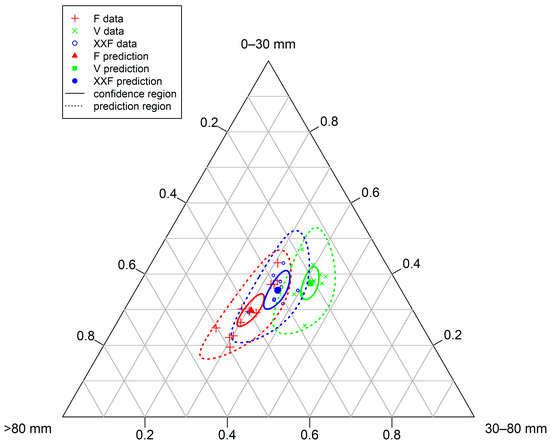
Figure 4. Prediction values and confidence and prediction regions for the particle size class distributions resulting from different cutting tool geometries.

The analysis of the ilr-residuals proves a multivariate normal distribution, with $p$-values of 0.67 and 0.89 for the Shapiro-Wilk test on univariate normality of each coordinate and $p$-values of 0.89 and 0.71 for Mardia’s Skewness and Mardia’s Kurtosis, respectively.

$R^2$ for the model is 0.57 and $R_{adj}^2$ is 0.54. These values are noticeably lower than those of the models for the throughput behavior and energy demand (see Reference [24]), which range from 0.73 to 0.87 for $R^2$ and from 0.67 to 0.81 for $R_{adj}^2$.

The lower coefficients of determination are reasonable since material fluctuations are likely to influence the material quality more than the process behavior, and sampling adds random noise (cf. Reference [7]). Considering the high expectable noise in processing experiments with real waste, and especially in shredding experiments (cf. Reference [24]), the model performance is satisfactory.

3.2. Discussion of the Method

The data from the particle size analyses were amalgamated to three discrete PSCs and then freed from the restrictions of the simplex by applying an ilr-transformation. The resulting model, the multivariate normal distribution of its residuals, and the consequent successful calculation of confidence and prediction regions prove the potential of this approach in terms of distribution-independent, mathematically correct empirical modeling of particle size distributions.

It is another potential application of ilr-transformations in the context of waste management, besides the application on waste compositions, in terms of sorting fractions (cf. Reference [33]). The method is a notable extension to the toolbox of chemical and process engineers in general, besides familiar approaches, like equivalent diameters or certain analytical distributions (see Section 1.1).

The discussed restriction of the method concerning zero-values is not an issue for the present data. When data include zeros, the potential impact of zero-handling techniques must be considered. These include amalgamations of compositional parts or zero-replacement (cf. Reference [42]).

Furthermore, the impact of the relative scale of ilr-transformed data must be kept in mind. Concerning the aim of the present work, it cannot be ignored, since the absolute values of the PCSs’ shares result in absolute waste masses, which are of interest. But the effect of the relative scale is low when the shares of all parts are of similar orders of magnitude, as is the case in this work (see Equation (23)). For other cases, calculations of weighted variances (cf. Reference [42]), for example, can be used to counteract the impact of the relative scale, if necessary. The relative scale can also be beneficial in other cases (as explained by Pawlowsky-Glahn et al. [27]), for example, where the share of trace elements in a chemical composition has a high impact.

The discussed issue of interpreting ilrs, is solved by graphical representation in this work. While this is a straightforward approach for three or fewer fractions, the question of how to represent more fractions arises. Graphic solutions include sets of ternary diagrams of two specific fractions and amalgamations of the others (cf. Reference [40]) and area plots (for the expected values, but not for confidence and prediction regions). Some other approaches include: The application of easier interpretable log-ratios (e.g., additive log-ratios or log-ratios incorporating amalgamations, cf. Reference [42]) at the cost of the exact representation of the variance structure in the data, or modeling non-transformed data, while incorporating potential issues with the restrictions of the simplex, particularly for calculating confidence and prediction regions.

Finally, the results in Figure 4 confirm the decision of Khodier et al. [24] to perform a Design of Experiments-based investigation, with multiple runs: the 95% prediction regions overlap even for the F and V unit. Hence, conclusions that contradict the findings in this work could be drawn when comparing only single runs of one hour.

3.3. Discussion of the Modeling Results

For the gap width and shaft rotation speed, no significant impacts on the produced PSDs were identified. In conclusion, either no such effects exist, or they are too small, compared to the residual variance in the data, to be detected based on the data at hand (resulting in so-called type II or β error). According to Biemann [51], no matter how small, any effect becomes significant if the amount of data is big enough. Hence, the order of magnitude of potential, non-identified effects is of interest. For the chosen limit $p$-value of 0.1 in the MANOVA, linear effects are preserved in the model if the 90% confidence regions of their extreme settings (which get smaller with more data) do not overlap. And potential effects are likely not to exceed the maximum distance of the borders of these regions.

Consequently, the confidence regions for the minimum and maximum settings of $w$ and $s$ at factor setting 0 for the other variables were plotted (see Figure 5), based on a linear model (see Equation (24)), to give a visual impression of potential type II errors. The residuals of these models also follow a multivariate normal distribution. Figure 5 shows, that $w$ influences the allocation to PSCs of 0 to about 13% of the product material, and $s$ influences 0 to about 9%, for average settings of the other factors.

$$\widehat{\overrightarrow{y}}={\mathrm{ilr}}^{-1}\left[\left(\begin{array}{c}{K}_{0000}^{\left(1\right)}\\ K_{0000}^{\left(2\right)}\end{array}\right)+\left(\begin{array}{c}{K}_{1000}^{\left(1\right)}\\ K_{1000}^{\left(2\right)}\end{array}\right)w+\left(\begin{array}{c}{K}_{0100}^{\left(1\right)}\\ K_{0100}^{\left(2\right)}\end{array}\right)s+\left(\begin{array}{c}{K}_{0010}^{\left(1\right)}\\ K_{0010}^{\left(2\right)}\end{array}\right)c_1+\left(\begin{array}{c}{K}_{0001}^{\left(1\right)}\\ K_{0001}^{\left(2\right)}\end{array}\right)c_2\right]$$

(24)

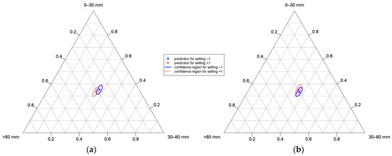
Figure 5. Ninety percent confidence regions for the minimum (−1) and maximum (+1) settings of $w$ (a) and $s$ (b), at factor setting 0 for the corresponding other factors of $w$, $s$, $c_1$ and $c_2$, based on the linear model from Equation (24).

Differences in the PSD, caused by the shaft rotation speed, would most likely be based on differences in the breakage of brittle materials in the waste, caused by the impact speed of the shaft’s teeth. Since the used machines are slow running shredders, the non-existence of such effects appears feasible. Furthermore, since potential impacts of this kind are most likely relatively small, the low share of brittle materials in mixed commercial waste (cf. Reference [7]) complicates their identification.

Concerning the gap width, considering the geometry of the cutting tools, a slight increase of the coarse fraction (>80 mm) would be reasonable due to falling through of uncomminuted particles between the teeth of the counter comb. But the non-significance of potential effects makes sense, considering that the breakage situation, according to Feyerer [52], does not change with the gap width for the F and XXF geometry and only slightly for the V geometry.

The influence of the cutting tool geometry is highly significant, with a factor $p$-value <10⁻⁵. As Figure 4 shows, it is largest, comparing the PSDs produced by the F and the V geometry. But the F and XXF geometries also differ significantly on a 95% confidence level. The results confirm expectations, considering the geometries (cf. Figure A1 and Table A1 in the Appendix A): The smaller axial gap between the counter comb teeth of the XXF geometry leads to a finer product, compared to the F unit. To be more precise, the share of the coarse fraction decreases in favor of the two other fractions.

Concerning the V geometry, the gap between the counter comb teeth is smaller than the gap of the F geometry. It is larger than the XXF geometry’s gap close to the shaft but gets much smaller with increasing distance. This smaller gap, combined with a comb system (cf. Reference [24]), leads to the finest product among the examined geometries—again, mainly in terms of an even lower share of coarse material compared to the XXF geometry.

Relating the results to the findings of Khodier et al. [24], the choice of a cutting tool geometry depends on the requirements of the process: The V tool produces the finest material of the three but at the cost of higher energy demand and smaller but steadier throughput.

Concerning the gap width and the shaft rotation speed, the standard operation with minimum gap widths and maximum shaft rotation speeds must be questioned: increasing the gap width is beneficial for the throughput and energy demand and hardly affects the throughput steadiness, according to Reference [24]. The shares of the PSCs chosen in this work (typical for SRF production) are not or only a little affected, with a maximum-likelihood influence on only about 3% of the material.

For the shaft rotation speed, the maximum likelihood influence of this non-significant factor on the PSD only concerns about 2% of the material, while the mass flow and energy demand show an optimum at about 84% and 80% of the maximum shaft rotation speed, respectively.

4. Conclusions

Multivariate multiple linear regression modeling was applied in this work on ilr-transformed PSC data from a Design of Experiments-based 32 runs coarse-shredding experiment with mixed commercial waste. A significant model, with an $R^2$ of 0.57 was found, identifying the cutting tool geometry as a highly significant influence on the PSD.

The gap width and shaft rotation speed were found not to be significant, with maximum-likelihood influences on 3% and 2% on the material, respectively. If the discussed potential type II errors are rated as economically relevant or other particle size classes are of interest, further data should be generated and analyzed. Otherwise, the PSD can be treated as invariant to these factors when optimizing the throughput and energy demand. Consequently, based on the new insights from this work, a much more efficient operation of mechanical waste processing plants can be reached. The influence of the cutting tool, on the contrary, is highly significant. Its choice depends on process requirements.

What was not investigated are selective influences on specific material fractions, e.g., metals or wood. The investigation of the PSDs of such fractions may give more detailed insights and lead to different conclusions on process parametrization. It is subject to further research, which can make use of the presented modeling methods.

Using the presented method requires an in-depth understanding of the implications of applying the ilr transformation. It is essential to avoid wrong interpretations, caused by the introduced relative scale or by zero-replacement practices, where necessary. Nonetheless, establishing such understanding is rewarding: in conclusion, the method has proven to be suitable for the distribution-independent modeling of PSDs. Hence, it is a valuable addition to the toolkit of engineers, dealing with particulate materials.

References

- Sarc, R.; Lorber, K.E.; Pomberger, R. Manufacturing of Solid Recovered Fuels (SRF) for Energy Recovery Processes. In Waste Management; Thomé-Kozmiensky, K.J., Thiel, S., Eds.; TK Verlag Karl Thomé-Kozmiensky: Neuruppin, Germany, 2016; pp. 401–416. [Google Scholar]
- Zhang, Y.; Banks, C.J. Impact of different particle size distributions on anaerobic digestion of the organic fraction of municipal solid waste. Waste Manag. 2013, 33, 297–307. [Google Scholar] [CrossRef]
- Luo, S.; Xiao, B.; Hu, Z.; Liu, S.; Guan, Y.; Cai, L. Influence of particle size on pyrolysis and gasification performance of municipal solid waste in a fixed bed reactor. Bioresour. Technol. 2010, 101, 6517–6520. [Google Scholar] [CrossRef] [PubMed]
- Sarc, R.; Curtis, A.; Kandlbauer, L.; Khodier, K.; Lorber, K.E.; Pomberger, R. Digitalisation and intelligent robotics in value chain of circular economy oriented waste management—A review. Waste Manag. 2019, 95, 476–492. [Google Scholar] [CrossRef]
- Sarc, R.; Seidler, I.M.; Kandlbauer, L.; Lorber, K.E.; Pomberger, R. Design, quality and quality assurance of solid recovered fuels for the substitution of fossil feedstock in the cement industry—Update 2019. Waste Manag. Res. 2019, 37, 885–897. [Google Scholar] [CrossRef]
- Leschonski, K. Windsichten [wind sifting]. In Handbuch der Mechanischen Verfahrenstechnik [Handbook of Mechanical Process Engineering]; Schubert, H., Ed.; John Wiley & Sons: Hoboken, NJ, USA, 2012; pp. 584–612. ISBN 3-527-30577-7. [Google Scholar]
- Khodier, K.; Viczek, S.A.; Curtis, A.; Aldrian, A.; O’Leary, P.; Lehner, M.; Sarc, R. Sampling and analysis of coarsely shredded mixed commercial waste. Part I: Procedure, particle size and sorting analysis. Int. J. Environ. Sci. Technol. 2020, 17, 959–972. [Google Scholar] [CrossRef]
- Möllnitz, S.; Khodier, K.; Pomberger, R.; Sarc, R. Grain size dependent distribution of different plastic types in coarse shredded mixed commercial and municipal waste. Waste Manag. 2020, 103, 388–398. [Google Scholar] [CrossRef]
- Feil, A.; Coskun, E.; Bosling, M.; Kaufeld, S.; Pretz, T. Improvement of the recycling of plastics in lightweight packaging treatment plants by a process control concept. Waste Manag. Res. 2019, 37, 120–126. [Google Scholar] [CrossRef] [PubMed]
- Gundupalli, S.P.; Hait, S.; Thakur, A. A review on automated sorting of source-separated municipal solid waste for recycling. Waste Manag. 2017, 60, 56–74. [Google Scholar] [CrossRef] [PubMed]
- Curtis, A.; Küppers, B.; Möllnitz, S.; Khodier, K.; Sarc, R. Digital material flow monitoring in waste processing—The relevance of material and throughput fluctuations. Waste Manag. 2021, 120, 687–697. [Google Scholar] [CrossRef] [PubMed]
- Möllnitz, S.; Küppers, B.; Curtis, A.; Khodier, K.; Sarc, R. Influence of pre-screening on down-stream processing for the production of plastic enriched fractions for recycling from mixed commercial and municipal waste. Waste Manag. 2021, 119. [Google Scholar] [CrossRef]
- Müller, W.; Bockreis, A. Mechanical-Biological Waste Treatment and Utilization of Solid Recovered Fuels—State of the Art. In Waste Management; Thomé-Kozmiensky, K.J., Thiel, S., Eds.; TK Verlag Karl Thomé-Kozmiensky: Neuruppin, Germany, 2015; pp. 321–338. [Google Scholar]
- Polke, R.; Schäfer, M.; Scholz, N. Charakterisierung disperser Systeme [Characterization of disperse systems]. In Handbuch der Mechanischen Verfahrenstechnik [Handbook of Mechanical Process Engineering]; Schubert, H., Ed.; John Wiley & Sons: Hoboken, NJ, USA, 2012; pp. 7–129. ISBN 3-527-30577-7. [Google Scholar]
- Wasserman, L. All of Statistics: A Concise Course in Statistical Inference; Springer: New York, NY, USA, 2013; ISBN 978-0-387-21736-9. [Google Scholar]
- Micula, G.; Micula, S. Handbook of Splines; Springer Netherlands: Dordrecht, The Netherlands, 1999; ISBN 978-94-010-6244-2. [Google Scholar]
- Scott, D.W. Multivariate Density Estimation; Wiley: New York, NY, USA, 1992; ISBN 9780471547709. [Google Scholar]
- Heumann, C.; Michael Schomaker, S. Introduction to Statistics and Data Analysis: With Exercises, Solutions and Applications in R; Springer: Berlin/Heidelberg, Germany, 2017; ISBN 978-3319461601. [Google Scholar]
- German Institute for Standardization. DIN 66143:1974-03, Darstellung von Korn-(Teilchen-)Größenverteilungen; Potenznetz [Graphical Representation of Particle Size Distributions; Power-Function Grid]; Beuth Verlag GmbH: Berlin, Germany, 1974. [Google Scholar]
- German Institute for Standardization. DIN 66145:1976-04, Darstellung von Korn-(Teilchen-)Größenverteilungen; RRSB-Netz [Graphical Representation of Particle Size Distributions; RRSB-Grid]; Beuth Verlag GmbH: Berlin, Germany, 1976. [Google Scholar]
- Sinnott, M.D.; Cleary, P.W. Simulation of particle flows and breakage in crushers using DEM: Part 2—Impact crushers. Miner. Eng. 2015, 74, 163–177. [Google Scholar] [CrossRef]
- Lee, H.; Kwon, J.H.; Kim, K.H.; Cho, H.C. Application of DEM model to breakage and liberation behaviour of recycled aggregates from impact-breakage of concrete waste. Miner. Eng. 2008, 21, 761–765. [Google Scholar] [CrossRef]
- Dong, K.; Esfandiary, A.H.; Yu, A.B. Discrete particle simulation of particle flow and separation on a vibrating screen: Effect of aperture shape. Powder Technol. 2017, 314, 195–202. [Google Scholar] [CrossRef]
- Khodier, K.; Feyerer, C.; Möllnitz, S.; Curtis, A.; Sarc, R. Efficient derivation of significant results from mechanical processing experiments with mixed solid waste: Coarse-shredding of commercial waste. Waste Manag. 2021, 121, 164–174. [Google Scholar] [CrossRef]
- Johnson, R.A.; Wichern, D.W. Applied Multivariate Statistical Analysis, 6th ed.; Pearson/Prentice Hall: Upper Saddle River, NJ, USA, 2007; ISBN 978-0-13-187715-3. [Google Scholar]
- Hand, D.J.; Taylor, C.C. Multivariate Analysis of Variance and Repeated Measures; Springer Netherlands: Dordrecht, The Netherlands, 1987; ISBN 978-94-010-7913-6. [Google Scholar]
- Pawlowsky-Glahn, V.; Egozcue, J.J.; Tolosana-Delgado, R. Modeling and Analysis of Compositional Data; John Wiley & Sons Inc.: Chichester, UK, 2015; ISBN 9781118443064. [Google Scholar]
- Pomberger, R.; Sarc, R.; Lorber, K.E. Dynamic visualisation of municipal waste management performance in the EU using Ternary Diagram method. Waste Manag. 2017, 61, 558–571. [Google Scholar] [CrossRef]
- Khodier, K.; Lehner, M.; Sarc, R. Multilinear modeling of particle size distributions. In Proceedings of the 8th International Workshop on Compositional Data Analysis (CoDaWork2019): Terrassa, 3–8 June 2019; Ortego, M.I., Ed.; Universitat Politècnica de Catalunya-BarcelonaTECH: Barcelona, Spain, 2019; pp. 82–85. ISBN 978-84-947240-1-5. [Google Scholar]
- Aitchison, J. The Statistical Analysis of Compositional Data. J. R. Stat. Soc. B 1982, 44, 139–177. [Google Scholar] [CrossRef]
- Egozcue, J.J. Isometric Logratio Tranformations for Compositional Data Analysis. Math. Geol. 2003, 35, 279–300. [Google Scholar] [CrossRef]
- Weise, D.R.; Palarea-Albaladejo, J.; Johnson, T.J.; Jung, H. Analyzing Wildland Fire Smoke Emissions Data Using Compositional Data Techniques. J. Geophys. Res. Atmos. 2020, 125, 139. [Google Scholar] [CrossRef]
- Edjabou, M.E.; Martín-Fernández, J.A.; Scheutz, C.; Astrup, T.F. Statistical analysis of solid waste composition data: Arithmetic mean, standard deviation and correlation coefficients. Waste Manag. 2017, 69, 13–23. [Google Scholar] [CrossRef]
- Chambers, J.M.; Hastie, T.J. Statistical Models. In Statistical Models in S; Chambers, J.M., Hastie, T.J., Eds.; Chapman & Hall: London, UK, 1993; pp. 13–44. ISBN 978-0-534-16765-3. [Google Scholar]
- Siebertz, K.; van Bebber, D.; Hochkirchen, T. Statistische Versuchsplanung [Design of Experiments]; Springer: Berlin/Heidelberg, Germany, 2010; ISBN 978-3-642-05492-1. [Google Scholar]
- Stat-Ease Inc. Optimality Criteria. Available online: https://www.statease.com/docs/v11/contents/advanced-topics/optimality-criteria/ (accessed on 26 May 2020).
- Dean, A.; Voss, D.; Draguljić, D. Design and Analysis of Experiments, 2nd ed.; Springer: Cham, Switzerland, 2017; ISBN 978-3-319-52250-0. [Google Scholar]
- Danish Standards Foundation. DS 3077 Representative Sampling—Horizontal Standard; Danish Standards Foundation: Charlottenlund, Denmark, 2013. [Google Scholar]
- Esbensen, K.H.; Wagner, C. Theory of sampling (TOS) versus measurement uncertainty (MU)—A call for integration. TrAC Trends Anal. Chem. 2014, 57, 93–106. [Google Scholar] [CrossRef]
- van den Boogaart, K.G.; Tolosana-Delgado, R. Analyzing Compositional Data with R; Springer: Dordrecht, The Netherlands, 2013; ISBN 978-3-642-36809-7. [Google Scholar]
- Khodier, K.; Lehner, M.; Sarc, R. Empirical modeling of compositions in chemical engineering. In Proceedings of the 16th Minisymposium Verfahrenstechnik and 7th Partikelforum (TU Wien, Sept. 21/22, 2020); Jordan, C., Ed.; TU Wien: Vienna, Austria, 2020; pp. 118–121. ISBN 978-3-903337-01-5. [Google Scholar]
- Greenacre, M. Compositional Data Analysis in Practice; CRC Press: Boca Raton, FL, USA, 2019; ISBN 978-1-138-31643-0. [Google Scholar]
- van den Boogart, K.G.; Tolosana-Delgado, R. Package ‘Compositions’ (Version 2.0-1). Available online: https://cran.r-project.org/web/packages/compositions/compositions.pdf (accessed on 13 January 2021).
- Stahel, W.A. Package Regr for an Augmented Regression Analysis. Available online: https://rdrr.io/rforge/regr/f/inst/doc/regr-description.pdf (accessed on 14 January 2021).
- Olson, C.L. On choosing a test statistic in multivariate analysis of variance. Psychol. Bull. 1976, 83, 579–586. [Google Scholar] [CrossRef]
- Pareto, A. Predictive R-Squared According to Tom Hopper. Available online: https://rpubs.com/RatherBit/102428 (accessed on 14 January 2021).
- Braun, W.J.; MacQueen, S. Package ‘MPV’ (Version 1.56). Available online: https://cran.r-project.org/web/packages/MPV/MPV.pdf (accessed on 14 January 2021).
- Wang, C.-C. A MATLAB package for multivariate normality test. J. Stat. Comput. 2014, 85, 166–188. [Google Scholar] [CrossRef]
- Mardia, K.V. Measures of multivariate skewness and kurtosis with applications. Biometrika 1970, 57, 519–530. [Google Scholar] [CrossRef]
- Korkmaz, S.; Goksuluk, D.; Zararsiz, G. Package ‘MVN’ (Version 5.8). Available online: https://cran.r-project.org/web/packages/MVN/MVN.pdf (accessed on 14 January 2021).
- Biemann, T. Logik und Kritik des Hypothesentests [Logic and criticism of the hypothesis test]. In Methodik der Empirischen Forschung [Methodology of Empirical Research]; Albers, S., Klapper, D., Konradt, U., Walter, A., Wolf, J., Eds.; Springer Fachmedien: Wiesbaden, Germany, 2007; ISBN 978-3-8349-0469-0. [Google Scholar]
- Feyerer, C. Interaktion des Belastungskollektives und der Werkzeuggeometrie Eines Langsamlaufenden Einwellenzerkleinerers [Interaction of the Load Collective and Tool Geometry of a Low-Speed Single-Shaft Shredder]. Master’s Thesis, Montanuniversitaet Leoben, Leoben, Austria, 2020. [Google Scholar]
Publisher’s Note: MDPI stays neutral with regard to jurisdictional claims in published maps and institutional affiliations. |
© 2021 by the authors. Licensee MDPI, Basel, Switzerland. This article is an open access article distributed under the terms and conditions of the Creative Commons Attribution (CC BY) license (http://creativecommons.org/licenses/by/4.0/).