Article

Modeling and Multi-Criteria Optimization of a Process for H2O2 Electrosynthesis

by
Martin von Kurnatowski
* and
Michael Bortz
Fraunhofer Institute for Industrial Mathematics ITWM, Fraunhofer-Platz 1, 67663 Kaiserslautern, Germany
*
Author to whom correspondence should be addressed.
Processes 2021, 9(2), 399; https://doi.org/10.3390/pr9020399
Submission received: 25 January 2021 / Revised: 12 February 2021 / Accepted: 14 February 2021 / Published: 23 February 2021
(This article belongs to the Special Issue Design and Optimization in Process Engineering)

Abstract

:
This article introduces a novel laboratory-scale process for the electrochemical synthesis of hydrogen peroxide (H 2 O 2 ). The process aims at an energy-efficient, decentralized production, and a mathematical optimization of it is presented. A dynamic, zero-dimensional mathematical model of the reactor is set up in Aspen custom modeler®. The proposed model constitutes a reasonable compromise between complexity and convergence. After thoroughly determining the reaction kinetics by adjustment to experimental data, the reactor unit is embedded in an Aspen Plus® flowsheet in order to investigate its interaction with other unit operations. The downstream contains another custom module for membrane distillation. Electricity appears as a resource in the process, and optimization shows that it reaches product purities of up to 3 wt.-%. Both the process optimization and the adjustment of the reaction kinetics are treated as multi-criteria optimization (MCO) problems.

1. Introduction

Electrochemical applications have undergone a remarkable increase in importance during the last decades due to the need for efficient modern technologies, e.g., in syntheses of substances or mobility, but also due to the rapidly evolving availability of new experimental and numerical tools for precise study and characterization of electrochemical systems [1]. One example of such an electrochemical device is the fuel cell (FC) for generation of electrical energy from oxidation of hydrogen or short-chained hydrocarbons like ethanol or methanol [2,3]. The most promising candidate for the large-scale production of hydrogen for use in fuel cells is the electrolyzer for water electrolysis [4], which is itself based on electrochemistry. Moreover, batteries are currently facing strong interest from researchers, since they are an essential component, e.g., in modern microelectronic devices, in electromobility and in energy storage. Latz and Zausch gave thermodynamically consistent theoretical descriptions of transport phenomena [5], reaction kinetics [6] and thermal aspects [7] in these devices. Another application of electrolysis is the conversion of carbon dioxide (CO 2 ) [8] to valuable products such as organic acids or short- and long-chained alcohols in order to reduce the global carbon footprint. A work realizing such a synthesis route experimentally to produce ethylene using copper(I) oxide catalysts can be found in [9].
The process introduced in this work comprises the oxygen reduction reaction (ORR) mechanism, with hydrogen peroxide (H 2 O 2 ) as the desired product. This important commodity chemical has a wide range of applicability in decentralized or industrial processes. In the chemical industry, it is synthesized via the anthraquinone process, delivering product purities of 1–2 wt%, which can be enhanced up to 70 wt% by downstream processing [10]. Due to its high oxidation potential, it is commonly used for treatment of waste water or bleaching of paper pulp or textiles [11,12]. Furthermore, it is employed extensively in the production of fine chemicals [13]. In the encymatic halogenation of the phenolic monoterpenes thymol and carvacrol to different products for anti-inflammatory, anti-microbial and anti-cancer applications, H 2 O 2 accompanied by the enzyme chloroperoxidase is used as a bio-catalyst [14]. Getrey et al. showed that the highest conversion rates are reached with electrochemical in-situ synthesis of H 2 O 2 directly in the active zone for the following reaction [15]. Thus, there are no transport problems for the catalyst as in the case of external injection of hydrogen peroxide. Since oxygen is used here as a reactant to produce H 2 O 2 , maximum efficiencies are achieved using gas diffusion electrodes [16] to avoid the problem of limited solubility of O 2 in the electrolyte.
Decentralized electrochemical production of H 2 O 2 has received growing interest from researchers in recent years. Yang et al. perceive this as part of a general trend [17]. They predict that the increased availability and decreased cost of renewable electricity will transform the chemical industry towards on-site production. This could lead to logistic challenges, e.g., if larger amounts of product have to be gathered. On the other hand, the decentralized approach has the potential advantages of more efficient energy conversion, easier product storage and lower capital expenditure according to Sehrish et al. [18]. In this respect, Li et al. recently stated that gas diffusion electrodes, such as the one used in the current work (see Section 2.3), are crucial to exploit the advantages of an electrochemical production of H 2 O 2 [19]. They quantitatively assessed their reactor with respect to energy consumption, production capacity, cost and long-term stability. They conclude that the technology is already feasible for on-site abatement of pharmaceutical residues in ground water. As for long-term stability, they report a life time of their electrode limited to about 46 days due to flooding of pores. In a real-world application, the electrodes need to be replaced before expiration to ensure a site-independent product quality.
Inspiration for modeling electrochemical reactors can be obtained from theoretical works on fuel cell research, the quantity of which is higher than that for electrolyzers. Since FCs convert substances into electric power, they can be considered as the inverse operation of electrosynthesis. Schultz et al. set up a rigorous, one-dimensional model of a direct methanol fuel cell using a Flory-Huggins activity model [20]. Later, the same group investigated the dynamic response of the system with respect to reaction kinetics [21]. The basic features to be covered by a model in any case are mass balances, material conversion, potential drops and membrane flows. In the case of spatial resolution (dim. > 0), local transport effects need to be described, too. They may be Knudsen diffusion or Maxwell–Stefan diffusion, the latter being governed by molecular friction in porous media [22], which is taken into account in [20]. Furthermore, Weinzierl and Krewer used numerical simulations to analyze the water management in direct methanol fuel cells [23,24]. For a more sophisticated approach, see e.g., [25], where a version of the 2D Navier–Stokes equations is solved for a mixture in order to investigate its coupling to chemical surface reactions via boundary conditions.
A mathematical model of an electrochemical cell for copper electrolysis, composed of 0D and 2D submodels, was given by Pohjoranta et al. [26], who validated their theoretical predictions by comparison to cyclic voltammetry measurements. However, this work is concerned with the overall process. Details about unit operations are secondary as long as their main dependencies are captured with reasonable accuracy. Hence, we stick to a 0D reactor model such as the one of Görgün et al. [27], who published a balance-based mathematical description of an electrolyzer with a proton exchange membrane (PEM), or the one of Argyropoulos et al. [28], who set up a semi-empirical 0D model of a direct methanol FC in a similar fashion. The aspired philosophy of the model equations is to aim for fast convergence while realistically reproducing measured data for the most important output quantities, i.e., the product weight fraction and the Faraday efficiency. This is additionally beneficial, because it does not imply a high number of transport coefficients as in the case of spatial resolution. Such coefficients (e.g., the binary Maxwell–Stefan diffusional coefficients) are often unknown in praxi due to the limited availability of experimental data for parameter estimation. However, it will be necessary to thoroughly determine the kinetics of the reaction mechanism under consideration.
A means of studying electrochemical reaction kinetics, which relies on experimental data, is the rotating ring-disk electrode (RRDE) system [29,30]. The method is based on the rotation of circular electrodes, inducing a forced flow to drag reactants to the electrode. Then, the detected electric currents at the disk and at the ring, with the latter being located at higher radii, contain information about the reaction kinetics. Yet, a micro-scale simulation is required in order to extract this information from experimental results. An application to determine electro-kinetic rate constants of the ORR mechanism at gold catalysts can be found in [31]. Recent reviews about catalysts for electrosynthesis of H 2 O 2 by oxidation of water can be found in [32,33]. Recently, two-dimensional RRDE simulations based on a finite-difference discretization were successfully adapted to corresponding measurements in a detailed and quantitative electro-kinetic study [34]. Such a way of determining parameters of a unit operation by simulations on a smaller scale can be considered as a part of a bottom-up modeling approach, as sketched in Figure 1. Alternatively, the kinetic parameters can be calculated by direct adjustment of the unit model to experimental data, as in this work.
The process model proposed in this article is set up in Aspen Plus V10®. However, this commercial flowsheet simulator does not provide a model of an electrochemical reactor as a unit operation and hence, an electrolysis cell model was implemented in Aspen custom modeler V10® (ACM) here. Note that this has been done before by Redissi and Bouallou [35], who performed an economic evaluation of a high-temperature co-electrolysis process for conversion of CO 2 /H 2 O to synthesis gas, based on simulations in Aspen Plus®. Apart from that, the process comprises a membrane distillation module [36] for separation of acidic components from the product solution in the downstream processing, which is neither available in Aspen Plus®. Implementations of such unit operations in Aspen Plus® can be found in [37,38]. A critical review on the modeling of membrane distillation technologies was given by Hitsov et al. [39]. A species-selective flow through a membrane is forced by the thermal gradient between a heated feed side and a cooler permeate side. The pores are hydrophobic and therefore the liquid phases from each side only partially penetrate the membrane. Material transport through the gas-filled segments of the pores is initiated by the difference in vapor pressures resulting from the different temperatures on both sides.
In most practical applications, electrochemical modules are part of higher-level processes with potential up- and downstream processing. However, the availability of studies considering electrochemistry on a process scale, i.e., in a coupled network of interacting modules rather than on the level of a unit operation, is limited. One of the few works on this topic was published by Karst et al. [40], who employed a multi-scale approach to design a fuel cell process with methane reforming in the upstream part for automotive application. Furthermore, Sanchéz et al. modeled an electrolysis process for hydrogen production in Aspen Plus® [41]. The current article contributes to this point by applying multi-criteria optimization (MCO) [42,43] with an adaptive scalarization scheme to a process containing an electrochemical reactor. The resulting optimal operating points apply for the entire process rather than a single device. For the MCO, Aspen Plus V10® is controlled via a programming interface. For this purpose, it offers an ActiveX automation server to be used within a VBA (visual basic for applications) code or a VB (visual basic) code. Previous work exploiting this interface for the optimization of separation processes can be found in [44,45]. The VBA code from [42] is used in the current work, since it already comes with an automated graphical user interface in MS Excel. Only the flowsheet simulator is exchanged here.
The model equations for the electrochemical reactor and the membrane distillation module are discussed in detail in Section 2.1 and Section 2.2 of this article. Subsequently, in 
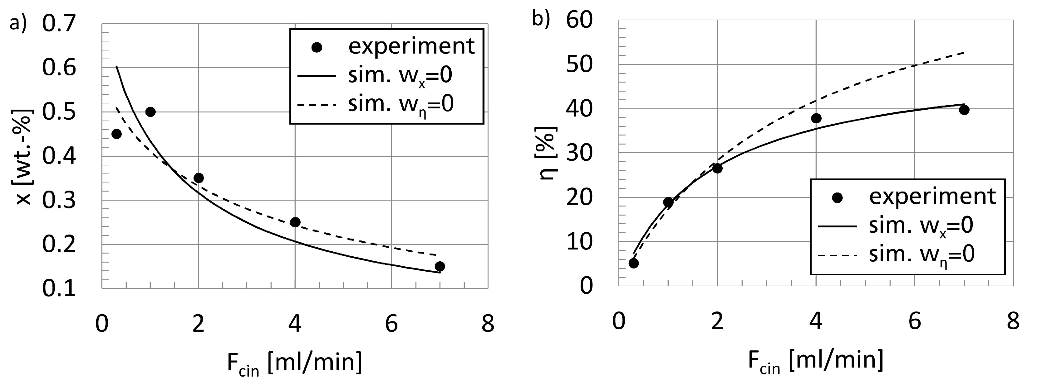
Section 3.1, particular attention is paid to the determination of electro-kinetic rate constants for the reactor model. This is realized here by direct adjustment of the model to experimental data, using MS Excel as a central interface coupling the simulation with an external optimization solver. Since two measured variables are available, the adjustment procedure is treated as an MCO problem, as suggested in [46]. A validation of the parametrized model equations is presented, too. Finally, according to the second modeling step in 
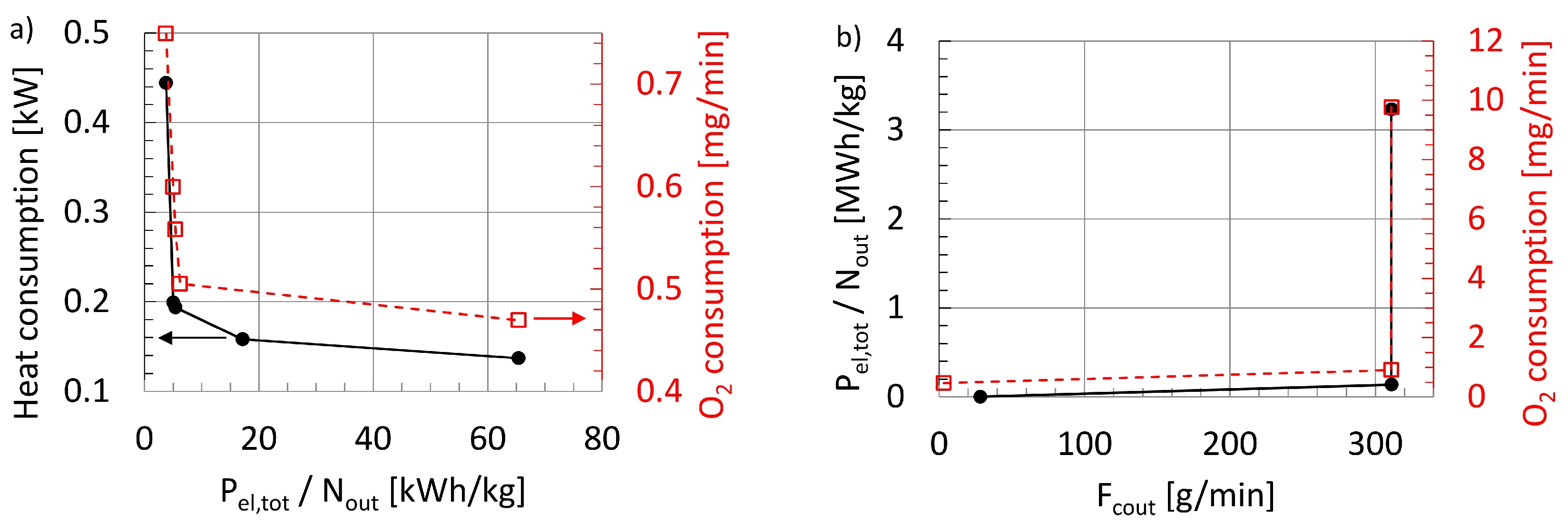
Figure 1, the adjusted model is embedded in a flowsheet for the entire process in Section 3.2. Pareto-optimal working points are then adaptively calculated [43,47], with particular respect to the electrical power required per product amount and the heat input.

2. Materials and Methods

2.1. Electrochemical Reactor Model

The electrochemical cell consists of a proton-exchange membrane (PEM), separating the two half cells, and two electrodes, each of which is separated from the PEM by a thin gap filled with electrolyte. Since the process incorporates a weakly soluble gas (oxygen in this case) as one of the educts, the reactor is designed with a gas diffusion electrode as cathode adjacent to a gas compartment. The model equations given in this section describe this as a zero-dimensional set-up. Yet, they contain several geometry parameters. The model captures time-dependent behavior, so that it can be applied in dynamic and stationary flowsheet simulations. The employed species are water, hydrogen peroxide, oxygen and hydrogen. In addition to that, sulfuric acid (H 2 SO 4 ) as solute in the water is considered, to become dissociated with the ions H 3 O + , HSO 4 and SO 4 2 . The models are implemented using Aspen custom modeler V10® with ENRTL-RK as the employed set of thermodynamic methods for the electrolyte.

2.1.1. Molar Balances in the Cathode Half Cell

The amounts of substances n c , i of species i in the cathode half cell are determined by the first-order differential equation
d n c , i d t = F c i n x c i n , i F c o u t x c , i + F g i n x g i n , i F g o u t x g , i + N m , i + j ν c , i j v c , j ( i H 2 O ) ,
where the last term corresponds to reactive conversions of substances. For an explanation of each quantity, refer to the list of symbols in Appendix A. The mole fractions in the cathode half cell and the gas compartment are related to the amounts of substances by
x c , i = n c , i / i = 1 N n c , i , x g , i = 0 ( i l i q ) ,
x g , i = n g , i / i = 1 N n g , i , x c , i = 0 ( i g a s ) .
From Equation (1), it can be seen that the balance is drawn around the cathode half cell and the gas compartment together. We neglect the solution of oxygen from the gas compartment in the bulk of the electrolyte in the cathode compartment, because the solubility of O 2 in water is only about 9 mg/L. Thus, at a moderate flow rate of 10 mL/min, there would be only 0.09 mg/min of dissolved oxygen leaving the cathode compartment. This can be neglected in the component balance because the system will be fed with about 5.3 g/min O 2 ( 0.09 mg/min). Evaporation of liquids into the gas compartment is neglected for similar reasons. Both effects would require a sub-model for mass transport through the gas diffusion electrode, which would be very difficult to parametrize realistically. So, the cost-benefit relation is insufficient for the type of overall process model that is set up here.
The concentrations in the bulk of the cathode half cell c c , i and at the cathode surface are given by the equations
c c , i = n c , i V c ,
D i δ c , i A c c , i s c c , i = j ν c , i j v c , j ( i g a s ) ,
c c , i s = H g , i p g , i ( i g a s ) ,
respectively. The concentrations c c , i s of the non-gaseous components at the surface are calculated from the linear relation (5), which is a local material conservation condition at the surface with a simplified version of Fick’s law in its differential form describing the molar flow rate through the boundary layer. It includes the assumption of spatially constant concentration gradients for the species diffusing towards the surface or away from it. Furthermore, it implies that the concentration profile adapts instantaneously to local concentration changes. The distinction between bulk and surface concentration in 0D is used as a feature to make the model more versatile by applying different values for the thickness of the boundary layer δ c , i . For water as the solvent, the limit δ c , H 2 O 0 is reasonably used (i.e., c c , H 2 O = c c , H 2 O s ). The concentrations of the gaseous components in the reactive zone (only O 2 in the process) follow from Henry’s law (Equation (6)) for solution of gases in liquids, since those species are fed to the reaction zone from the gas compartment side.
In order to match the number of equations and the number of calculated variables, another equation for the determination of F c o u t is required. For a realistic description of the reactor, it is necessary to consider the Equation
V c = i l i q V c m , i n c , i ,
requiring the gap in the half cell to be steadily brimfull with liquid. However, with this equation used to calculate F c o u t , the model converged poorly in our tests. Instead, the equation is used to determine n c , H 2 O , and hence, the dynamic Equation (1) is not used for water. To obtain an equation for F c o u t , Equation (7) is differentiated with respect to time, and the resulting expression for n ˙ c , H 2 O is set equal to its analogue arising from the unused molar balance (1) for water. This yields the incompressibility condition
0 = F c i n x c i n , H 2 O F c o u t x c , H 2 O + N m , H 2 O + j ν c , H 2 O , j v c , j + 1 V c m , H 2 O i H 2 O i liq V c m , i n ˙ c , i
(with n ˙ c , i in the last sum from Equation (1)) for calculation of F c o u t . Thus, the molar balance for water is contained implicitly in the equations. F g o u t follows from the phenomenological relation
F g o u t = K v V g m ρ 0 ρ g p g p 0 1.0
with a slight pressure drop being assumed across the outlet valve of the gas compartment.

2.1.2. Molar Balances in the Anode Half Cell

The balance equations on the anode side are analogue to the cathode balances, except for the gas compartment, which does not exist for the anode half cell. The molar component balance for the anode reads:
d n a , i d t = F a i n x a i n , i F a o u t x a , i N m , i + j ν a , i j v a , j ( i H 2 O ) ,
with the mole fractions given by
x a , i = n a , i / i = 1 N n a , i .
Again, the bulk and surface concentrations are obtained from
c a , i = n a , i V a ,
D i δ a , i A c a , i s c a , i = j ν a , i j v a , j ,
with c a , H 2 O = c a , H 2 O s . In contrast to the cathode side, dissolved oxygen emerging from oxidation of water occurs on the anode side in the process. The anode half cell is supposed to be entirely filled with liquid, too:
V a = i l i q V a m , i n a , i ,
meaning that oxygen bubble formation is not considered here. Such bubbles increase the overpotential by blocking active surface sites. Nouri-Khorasani et al. report changes in the overpotential of 28…43 mV in this respect [48]. Neglecting this effect is reasonable because the cell in this article works at about 1.6 V ( 43 mV) under moderate operating conditions. The molar balance (10) for water is used only implicitly during the derivation of the incompressibility condition
0 = F a i n x a i n , H 2 O F a o u t x a , H 2 O N m , H 2 O + j ν a , H 2 O , j v a , j + 1 V a m , H 2 O i H 2 O i liq V a m , i n ˙ a , i
for calculation of F a o u t .
There are two contributions to N m . The oxonium ions H 3 O + are the only charged particles traversing the PEM. Moreover, water is the only non-charged component being conducted through the membrane by electro-osmotic drag. Then, we have
N m , H 3 O + = I F ,
N m , H 2 O = I F λ ,
N m , i = 0 ( i H 3 O + , H 2 O )
with the drag coefficient λ .

2.1.3. Reaction Kinetics and Voltage

The electric current I j across the electrode surface resulting from reaction j is calculated using the Butler–Volmer equation [6,49]:
I j = A F l j k j c o x , j s e l j α F R T ( E E j 0 ) c r e d , j s e l j ( 1 α ) F R T ( E E j 0 ) .
The sum of this equation over all electrochemical reactions for one electrode yields the condition
I = j I j ,
which determines the electrode potential E for the case of galvanostatic operation. Equation (20) only holds if all occurring electrochemical reactions are known. Equation (19) enables us to give the Faraday efficiencies
η j = I j I
explicitly. Note that these Faraday efficiencies are not identical to the η usually resulting from experiments, where the molar flow rate of the product species is measured and divided by its theoretical maximum according to the electric current. These experimental values correspond to a species rather than a reaction. They are averaged over all reactions involving the species, and they become equal to η j in case of only one reaction, or more precisely, in the case where the respective component occurs only in reaction j. Apart from that, the electric reaction currents I j are used to calculate the reaction rates from Faraday’s law of electrolysis:
v j = I j l j F .
The formal potential E j 0 is calculated from the Nernst equation, and the equilibrium potential E j e q , i.e., the electrode potential in case of only reaction j and zero electric current, is derived from E j 0 accordingly:
E j 0 = E j o R T l j F i ln ( γ i j s ) ν i j ,
E j e q = E j 0 R T l j F i ln c i j s c 0 ν i j .
Values for potentials are given with reference to the standard hydrogen electrode (SHE) in this work. Equations (19)–(24) are evaluated separately for each electrode. However, they are only written down here once, because they are the same in both cases.
To determine the overall voltage drop over the cell, we require the Ohmic voltage drop
U O h m = I ( R l i q + R m )
with the resistance of the electrolyte in the gaps and the resistance of the membrane:
R l i q = d a + d c σ l i q A ,
R m = d m σ m A .
Furthermore, the overpotential associated with reaction j is defined as
E j o v e r = E E j e q ,
which is, just like the Faraday efficiencies from (21), a measure of efficiency for the cell.
In the literature, the overall cell voltage U is usually composed of the open circuit voltage U 0 , the overpotentials and the Ohmic losses. However, in the case of multiple active reactions, it is not straightforward to calculate U 0 and the total overpotentials at each electrode. Using Equations (23) and (26) from [20] instead, U can be written in terms of E a and E c :
U = U O h m + E c E a ,
where the potential difference E c E a consists of the open circuit voltage and the total overpotentials. This form can be evaluated because E a and E c , which are not reaction-specific, are calculated from (19) together with (20).
Finally, the electric power consumption of the cell is
P e l = U I .
In this convention, the electric current I has a positive algebraic sign. The applied electrical power enables the necessary increase in the Gibbs free energy and thus, the conversion of chemicals. However, it partly gets lost due to Joule heating and overpotentials, which are caused by polarization effects at the electrodes [28,49].

2.1.4. Reactions

The model equations given so far are generic in the sense that they do not correspond to a particular electrochemical reaction mechanism. In order to refer to the process of H 2 O 2 production, the following reactions were implemented together with the model.
Cathode:
O 2 + 2 H 3 O + + 2 e k 1 2 H 2 O + H 2 O 2
O 2 + 4 H 3 O + + 4 e k 2 6 H 2 O
H 2 O 2 + 2 H 3 O + + 2 e k 3 4 H 2 O
Anode:
6 H 2 O k a 4 H 3 O + + 4 e + O 2
The desired reaction (31) is the oxygen 2-electron reduction to hydrogen peroxide, which is often accompanied by the oxygen 4-electron reduction to water (Equation (32)) and a subsequent reduction of H 2 O 2 (Equation (33)). Together, (31)–(33) constitute the oxygen reduction reaction (ORR) mechanism [30,31,50]. At the counter electrode, the anodic reaction of water electrolysis (Equation (34)) is used for the production of H 3 O + . These are the four active reaction channels for the process.

2.2. Membrane Distillation Model

The process includes downstream processing employing a module for membrane distillation to remove the added acid from the product solution. This separation process is principally based on differences in the chemical potential of species i on both sides of the membrane. Assuming the trans-membrane flux N m , i to be proportional to this difference, it can be expressed as [51]
N m , i = B i p i , f 0 γ i , f x i , f p i , p 0 γ i , p x i , p ,
neglecting any non-ideal behavior of the gas phases on each side. The transport coefficients B i depend on the membrane thickness and on how efficiently species i is transferred through the membrane. The flux (35) is forced by a thermal gradient across the membrane. The feed stream to the feed side of the module is heated to a temperature T f well above the feed temperature T p on the permeate side. Consequently, the saturation vapor pressure p i , f 0 of species i in the feed side of the pores is higher than the saturation vapor pressure p i , p 0 of species i in the permeate side of the pores. The solutions on each side penetrate the membrane only to a certain extent but never reach the liquid coming from the other side due to the hydrophobic design of the pores. The difference in vapor pressures on each side causes a material flux through the gas-filled section of the pores. Again, the vapor pressures of the liquid components and the activity coefficients γ i , f , γ i , p at compositions x i , f , x i , p are obtained using the corresponding methods from Aspen’s ENRTL-RK set. The pressures of gaseous species are calculated using Henry’s law.
The outlet compositions x o u t , i , f , x o u t , i , p are determined by the component balances
F o u t , f x o u t , i , f = F i n , f x i , f N m , i ,
F o u t , p x o u t , i , p = F i n , p x i , p + N m , i
on the feed and the permeate side, respectively, and the outlet flow rates F o u t , f , F o u t , p follow from the sum of Equation (36) and (37) over all components, exploiting the summation conditions:
F o u t , f = F i n , f i N m , i ,
F o u t , p = F i n , p + i N m , i .

2.3. Experimental Details

Experimental data were generated in order to adjust and validate the model. The measurements were conducted with the real electrochemical cell, which had a cross-sectional area of A = 100 cm 2 . The thicknesses of the anode and cathode compartment are d a = 7 mm and d c = 1.2 mm, respectively, and the corresponding compartment volumes are calculated accordingly as V a = d a A = 70 cm 3 and V c = d c A = 12 cm 3 . The half cells are separated by a fumasep® F-10120-PK proton exchange membrane (PEM). The cathode was made of a hydrophobized commercial Freudenberg H23C8 gas diffusion layer, which was sputtered with platinum as catalyst in order to obtain a gas diffusion electrode. The gas compartment is fed with 175 Nml/min synthetic air. For the anode half cell, an electrolyte solution of 2 mol/L H 2 SO 4 in water is used, which is fed with a rate of 70 mL/min and which is recycled after it passed the cell. The experiments were conducted at room temperature (about 22.5 C in the laboratory), and no temperature control or external cooling was applied to the cell. Furthermore, the measurements were executed using galvanostatic operation with an electric current of I = 2.37 A. Due to the low values of the product purity x (below 1 %), the corresponding relative measurement error is rather large (up to 50 %). Thus, values of model parameters derived from the measured data are considered as estimates.

3. Results and Discussion

3.1. Model Adjustment

In this subsection, the reactor model is adjusted to the experimental data. Sensitivity analyses of the model performed in Aspen Plus® showed that the electro-kinetic parameters from the Butler–Volmer Equation (19) have the highest impact on the output quantities of the model and hence, they are chosen as free variables in an optimization problem designed to adjust the model to the measurements. The applicability of the determined reaction kinetics after a potential upscaling of the process then depends on how realistically the other model parameters are chosen. Some of the remaining input parameters can be determined from literature, e.g., the standard potentials under standard conditions E j o . Table 1 summarizes the parameter values used in the model adjustment of the electrochemical reactor. At the cathode, reactions (31)–(33) are active and they are enumerated consecutively, i.e., the reaction index j (used e.g., for α j and E j o ) is 1 for the reaction from (31), 2 for (32) and 3 for (33). At the anode, the water electrolysis reaction (34) is active. The parameters d m , σ m concerning the membrane are taken from the data sheet provided by the manufacturer (see Table 1). The reference quantities are set to p 0 = 1.01325 bar, c 0 = 1 mol/L and ρ 0 = 1 g/cm 3 . The true component approach is used to specify the acid concentration, i.e., only the mole fraction of H 2 SO 4 is entered and the employed property methods provided by Aspen calculate the corresponding ionic concentations. All feed temperatures and pressures to the reactor are set to 22.5 C and 1.01325 bar, except for the feed pressure to the gas compartment, which is set to 1.02 bar. The gas compartment is fed with pure oxygen in the simulation, and the associated feed rate is set to 20 % of the experimental value, which is the percentage of oxygen in synthetic air. Still, there are some model parameters to be estimated, e.g., the electro-osmotic drag coefficient is chosen as λ = 6 from experimental experience. In previous work for the ORR mechanism at PdAu 3 surfaces, the charge transfer coefficients were calculated [34]. Here, they must be in the same order of magnitude since the E j o do not differ.
The model parameters obtained from model adjustments here result from the solution of a least squares problem. For the electrochemical reactor, the product purity x and the Faraday efficiency η were measured as functions of the feed rate to the cathode half cell. The objective function f to be minimized is the weighted sum over all normalized and squared differences between the measured values and the values predicted by the model at given cathode feed rate F c i n :
f = w x S x + w η S η ,
with S x , S η given by
S x = l = 1 N x x s i m , l x e x p , l x ¯ e x p 2 ,
S η = l = 1 N η η s i m , l η e x p , l η ¯ e x p 2 .
The terms are normalized to their mean experimental value. Here, the simulated Faraday efficiency is calculated as in the experiments, i.e., the product purity x is recorded, multiplied by the set point for the flow rate F c i n and finally divided by the theoretical maximum I / ( 2 F ) for the case without side reactions:
η s i m = x F c i n I / ( 2 F ) .
The solver NLPQLP from the Schittkowski suite [53] is used to minimize f by varying the optimization variables k 1 , k 2 and k 3 .
Since electro-kinetic rate constants may vary by many orders of magnitude [49], they are replaced using the nonlinear transformation
k j = 10 b j
and the b j are used as optimization variables instead. This way, the optimization solver calculates steps in a logarithmically scaled design space and it does not need to distinguish between steps of different orders of magnitude. Without this transformation, no meaningful results could be found. Table 2 shows the employed starting values and boundaries for the optimization variables.
Particular attention needs to be paid to the different convergence parameters when working in the framework of flowsheet optimization. The error tolerance of the optimization solver and the accuracy of gradient calculations must be less strict than the accuracy of the simulation. Otherwise, the information the solver is looking for in the function evaluations will simply disappear in numerical noise. Here, the tolerance of NLPQLP is set to 10 3 , the relative accuracy of the gradients is 10 4 and the flowsheet tolerance is 10 8 . The latter is used as accuracy requirement for mass balances, flash calculations and for the system of equations itself, which is solved in equation-oriented mode.
A common choice for w x , w η is the reciprocal variance of the corresponding experimental data [54], ensuring that more precisely measured quantities are granted more impact on the objective function. However, the variances are often unknown, as is the case here, too. Hence, the weighting factors can be chosen out of a continuum between the extreme compromises w x = 0 , w η > 0 and w x > 0 , w η = 0 , where the optimization variables are adapted to only one quantity, respectively. We use the sandwiching algorithm [43] to adaptively determine distinct sets of weighting factors, for each of which the optimization problem described above is solved. The result is a finite number of solutions, each corresponding to a different estimate for the k j . These points represent a Pareto set [47] with well-defined sandwiching quality in the objective space spanned by the criteria S x and S η . A similar procedure has also been presented in [46] for solving reconciliation problems.
Aspen Plus V10® is coupled to the NLPQLP solver and the sandwiching subroutines via MS Excel. A VBA code is used to manage the data transfer, and a self-designed (Excel-based) graphical interface is used for problem specification and automated formatting of results. The framework is similar to the one published in [42], except for CHEMCAD as a flowsheet simulator being replaced by Aspen here. The applied HappLS class from the Aspen Plus GUI 36.0 Type Library exposes all required properties and methods to access flowsheet data from within VBA.
Figure 2 shows the Pareto frontier of the MCO problem for adjustment of the electrochemical reactor model to measured data displayed in the objective space spanned by the sums S x and S η . Within the given approximation quality (see bottom of Table 1), this frontier is represented by the calculated Pareto points and the straight lines connecting them. It is the set separating the feasible and infeasible parts in the objective space. In the plot, the extreme compromises are marked corresponding to w x = 0 (bottom right) and w η = 0 (top left). For all six calculated points, the results including the respective weighting factors w x , w η determined by the sandwiching algorithm are listed in Table 3.
A comparison of the experimental data to the predictions of the adapted models is exhibited in Figure 3. The measured data represented by black dots are displayed as a function of the feed rate to the cathode half cell F c i n . The extreme compromises w x = 0 , w η = 0 corresponding to solutions 1 and 2 in Table 3 were chosen for the plot. I.e., the b j for the two solutions were inserted into Equation (44) to obtain the respective electro-kinetic rate constants k j for utilization in the cell model. Subsequently, the models were solved for 40 equidistant values of F c i n in the interval 0.3…7 mL/min, in order to reach a quasi-continuous representation for the lines in Figure 3. For both parametrizations, the model from Section 2.1 achieves a reasonable approximation of the experimental data. The simulation results for w x = 0 (solid line) deviate more strongly from the measurements for x, especially at low feed rates, and the simulation results for w η = 0 agree less well with the measurements for η , particularly at larger feed rates. This is the expected result because e.g., for w x = 0 , the deviations accumulated in S x from (41) are not taken into account in the objective function f from (40). Hence, the corresponding measurement points cannot force the curve to pass them by more closely in the optimization procedure. For F c i n between 0.3…2 mL/min, the model reproduces the experimental values for η almost exactly for both parametrizations. The results of solution 1 ( w η = 0 ) are chosen for the model used in the subsequent section about process optimization, because there, a more accurate prediction of the product purity is desired, since the considered criteria partly depend on x, but not on η . Using j 0 = F k ( c O b ) 1 α ( c R b ) α [49], an exchange current density of j 0 5 μ A/cm 2 can be found for the corresponding kinetic parameters. This is comparable to the lowest values found in [55] for the Pt/Nafion interface.

3.2. Process Optimization

3.2.1. Flowsheet Parameter Settings

Figure 4 shows the flowsheet of the process for the electrosynthesis of H 2 O 2 introduced in this work. The reactor model described in Section 2.1 and parametrized in Section 3.1 is integrated as the core unit EC (1). The design specifications ACICONTA and ACICONTC control the acid feeds ACIFEEDA and ACIFEEDC, such that the respective direct feeds FIRI-16 and FIRI-18 to the anode and cathode half cells have H 2 SO 4 concentrations of 0.5 mol/L. Both acid feed streams have 10 wt.-% H 2 SO 4 . Accordingly, H2OCONTA and H2OCONTC control the water feed streams H2OFEEDA and H2OFEEDC. For the cathode, this flow rate is variable, and for the anode it is set to 0.1 kmol/h. Due to the anode recycle loop, the streams ACIFEEDA and H2OFEEDA are reduced to very small flow rates by the solvers, because most material is recycled. H 3 O + and H 2 O can leave this loop through the PEM in EC, and the gas separation O2SEP (3) was inserted to remove all oxygen emerging from reaction (34) at the anode, which would otherwise become highly accumulated. HEAT1 (4) establishes a variable temperature difference between both sides of the membrane distillation module MD1 (2). PFCONT varies the stream PERMFEED, such that stream AUX05 has a total flow rate of 0.01 kmol/h. The flash H2O2CONC (4) for concentration of the product solution is specified with a temperature of T c = 110 C and a vapor fraction of y c = 0.5 mol/mol. H 2 O 2 enters the downstream recycle loop through the membrane in MD1 and leaves it as the high-boiling component through the liquid outlet TOFPROC from H2O2CONC. Both cooling units diminish the temperature to 22 C and all pumps raise the pressure by 5 hPa except for P04, which is specified to a 10 hPa pressure increase. The oxygen feed O2FEEDC has a flow rate of 0.01 kmol/h at 22 C and 1.025 bar, which is decreased to 1.02 bar by the valve V3. All other feeds have a pressure of 1.01325 bar, also at 22 C. The B i for MD1 are taken as 1 kmol/(bar · h), except for water and H 2 O 2 , for which they were estimated to B H 2 O = 0.01 kmol/(bar · h) and B H 2 O 2 = 7 kmol/(bar · h) from experimental data. The geometry, electro-kinetic and membrane parameters, as well as the estimated parameters for EC, are taken as in Table 1, and the electro-kinetic rate constants for the Butler–Volmer equation are derived from Table 3 (row with w η = 0 ) using Equation (44). The flowsheet simulation takes into account the downstream section, recycle streams and the impact of the interactions between unit operations. With all of its structure, specification and parametrization, it is supposed to be the digital twin of the laboratory process, capable of replacing experiments by numerical simulations for finding optimal points of operation.

3.2.2. Flowsheet Convergence

The flowsheet is solved in sequential-modular mode. Two steps turned out to be crucial in order to obtain convergence. First, O2SEP had to be inserted for the above-mentioned reason. Second, the design specifications were nested inside the loops converging the tear streams FBA1 and AUX04. Otherwise, the tear streams cannot converge, because, e.g., the anode recycle loop would have to be closed with the initial flow rate of H2OFEEDA, which is far too large for the amount of substance in the loop to remain finite. Tear streams as well as design specifications are converged with Broyden solvers. The relative tolerance for AUX04 is 10 4 , while it could be reduced to 10 8 for FBA1. The accuracies of the design specifications in the upstream processing are 10 5 , and for PFCONT it is 10 3 . The error tolerances for flash convergence, entropy balance and for fugacity calculations are set to 10 8 , and the accuracy of mass balances is 10 4 .

3.2.3. Multi-Criteria Optimization Problem

For the optimization problem, the solver accuracy was set to 10 3 , numerical derivatives were evaluated using a relative perturbation of 3% and the quality of the sandwiching approximation was 1.05. Table 4 provides an overview over the MCO problem designed to analyze the process and to calculate Pareto-optimal working points for it. The optimization variables are I, F c i n and the temperature T M D of the stream to the feed side of the membrane distillation unit MD1. The latter quantity is a specification for HEAT1. I is varied in the interval 0.5…10 A. At I = 0.5 A there is almost only 0.05 wt.-% H 2 O 2 left in the main outlet TOFPROC, and we do not wish to go below that. Apart from that, it should be noted that for I as high as 10 A, a notable production of H 2 , which is not considered here, sets in in the real system. Furthermore, at such high electric currents, external cooling of the reactor is required, which is not considered here, either. The boundaries for F c i n are 0.01…1 kmol/h according to a reasonable interval of 3 300 mL/min. T M D is kept between 23…98 C, so that the feed temperature for MD1 is always higher than the permeate temperature but without evaporating the solution. The optimization solver works with T M D measured in units of 10 C because then the actual optimization variable is O ( 1 ) within its boundaries, which turned out to be more stable. Among the five objectives, three quantities have not been introduced yet: the overall electric power consumption P e l , t o t is taken as the sum of the cell power P e l and the powers of all pumps, and the ratio of this quantity to the component flow rate N o u t of H 2 O 2 in TOFPROC is a measure for the electrical energy dissipated per kg peroxide output. P e l takes its lowest value of 0.4 W for I = 0.5 A, F c i n = 0.01 kmol/h. x o u t is the overall product purity, i.e., the mass fraction of H 2 O 2 in the main outlet. The heat consumption is the sum of the net duties of HEAT1 and COOL1 for separation of acidic components and the net duties of the flash H2O2CONC and COOL2 in the recycle loop for product concentration. The O 2 consumption is taken as the mass flow rates of O2FEEDC minus O2OUTA and O2OUTC, since the two latter streams are considered as recycled.

3.2.4. Multi-Criteria Optimization Results and Discussion

The highest H 2 O 2 purities in TOFPROC were found at about 3 wt.-%. The outcome of the Pareto approximation shall be discussed here within the context of two-dimensional projections in the objective space. Figure 5a shows such projections for the heat consumption and the O 2 consumption of the entire process with P e l , t o t / N o u t on the horizontal axis. The data sets for Figure 5 are given in Table 5. Within the given approximation quality, the plotted lines represent the boundary between feasible and infeasible regions. Resulting points appearing as dominated in the projections (i.e., points where an improvement in both objectives is possible without becoming infeasible) in the corresponding projection have been removed from the plots. In Figure 5a, the transition from high to low heat and O 2 consumptions while simultaneously worsening the ratio P e l , t o t / N o u t along the Pareto sets in this diagram is achieved by reducing the feed rate to the cathode half cell from 0.09 to 0.01 kmol/h and by lowering T M D . Of course, this will lead to smaller heat consumptions, but it also results in less H 2 O 2 crossing the membrane in MD1 and hence in lower values of N o u t .
Very sharp bends in the Pareto frontiers are found in Figure 5b. For the O 2 consumption, the bending point in the bottom right can be reached from the point in the top right, mainly by decreasing the electric current from 2.38 to 0.5 A. This drastically reduces the amount of oxygen converted in electrochemical reactions. In fact, both objectives on the vertical axes can be decreased by more than an order of magnitude in this range, with almost no reduction in F c o u t . Such interesting regions are sought after by and can only be found using MCO, while the sandwiching algorithm prevents an unnecessary amount of points being calculated in these intervals. Mind that only two criteria are regarded in this reflection. e.g., x o u t drops significantly with decreasing I. From the solution in the bottom left of Figure 5b, the bending point is reached by increasing F c i n . This notably improves F c o u t , while the other two objectives in the projection worsen only marginally.
In order to assess the relation of electrical and thermal energy consumption, the reactor and the membrane distillation module are compared. At moderate operating conditions ( I = 2.37 A, F c i n = 0.025 kmol/h, T M D = 70 C), the cell power P e l is 3.84 W. It mainly depends on the electrical current and is increased to 56.87 W by increasing I to its upper boundary at 10 A. The heat for membrane distillation is injected in HEAT1. Under the moderate conditions just mentioned, this heater operates at a thermal input of 25.59 W. This heat input depends on T M D , and it is increased to 40.54 W by increasing T M D to its uppper boundary at 98 C. Hence, depending on the operating conditions, P e l can be smaller or larger than the energy required for membrane distillation, and its range comprises that of the heat input in HEAT1. The overall heat consumption (see Table 5) exceeds the electrical power, but such a contribution also exists in the conventional anthraquinone process.
In Table 5, there are several non-identical values of T M D very close to 70 C. This was investigated using a sensitivity analysis in the range T M D = 69.9 70.1 C with I = 0.5 A and F c i n = 0.01 kmol/h. F c o u t and the O 2 consumption do not depend on T M D , the latter because there is no oxygen in the downstream. P e l , t o t / N o u t does not vary notably in this range. However, x o u t as well as the heat consumption both vary by about 0.2% in this range. On the one hand, this variation is large enough so that, together with the given solver tolerance of 0.001, our algorithm can distinguish between the respective values in the table and they do not result from numerical noise. On the other hand, the variation is small enough for a robust implementation of the Pareto-optimal operating points in the real process. The challenge will then be to accurately establish the optimal temperature all over the feed side of the membrane in MD1.

4. Conclusions

This work introduces a process for electrosynthesis of H 2 O 2 and focuses on its modeling and multi-criteria optimization. The proposed model equations for the required custom units pursue the goal of rapid convergence and a reasonable mathematical mapping of the main output quantities, particularly the product purity but also the Faraday efficiency. For calculation of the outlet flow rates of the reactor, a numerically stable incompressibility condition is derived. The Butler–Volmer kinetics are determined from adjustment to experimental data, which is realized by solving an MCO problem, since it is not clear in general how to weight different measured quantities against each other. The model is implemented in Aspen custom modeler®, and its validated form is embedded in an Aspen Plus® flowsheet. For the application of MCO to both, model adjustment as well as electrosynthesis on a process level, the availability of studies is limited so far.
The Pareto set obtained from MCO can be exploited by process operators for a quick and simple selection of efficient working points without the need for further simulations, and especially without time-consuming experiments. The MCO results show that the product purities of the process introduced here are higher than those of the anthraquinone process (before downstream). Hence, the proposed process is a promising approach to sustainable production of hydrogen peroxide. However, the product flow rates in the range of several mL/min cannot compete with the industrial process. However, they need not, because the process considered here is designed for decentralized applications. Nevertheless, the product amount should be increased in future work. In this respect, upscaling cannot be the (only) solution because the process is supposed to remain decentralized. However, stacking multiple electrochemical cells can be one way to achieve higher product flow rates (at the cost of more energy input of course).

Author Contributions

Conceptualization, M.v.K. and M.B.; methodology, M.v.K.; software, M.v.K.; validation, M.v.K.; writing—original draft preparation, M.v.K.; writing—review and editing, M.v.K. and M.B.; visualization, M.v.K.; supervision, M.B.; project administration, M.v.K. and M.B.; funding acquisition, M.B. All authors have read and agreed to the published version of the manuscript.

Funding

This research was funded by the Fraunhofer Society within the Lighthouse Project “Electricity as a Resource”. The APC was funded by the Fraunhofer Society.

Institutional Review Board Statement

Not applicable.

Informed Consent Statement

Not applicable.

Data Availability Statement

All data required to reproduce the results presented in this study can be found in the article.

Acknowledgments

Our gratitude goes to Carsten Cremers and Jan Meier from the fuel cell group at Fraunhofer ICT for the measured data and a lot of information about electrochemical systems. Stimulating discussion about the basic principles of membrane distillation with Dusan Boskovic from the “Chemical process development and flow chemistry” group at Fraunhofer ICT is gratefully appreciated. In addition to that, we are much obliged to Johannes Neuhaus from BASF SE for helping with the convergence properties of the flowsheet simulation for the process. Useful support in the MCO procedure by Jens Babutzka from SAP SE Germany is thankfully acknowledged.

Conflicts of Interest

The authors declare no conflict of interest.

Abbreviations

The following abbreviations are used in this article:
ACMAspen custom modeler®
FCFuel cell
MCOMulti-criteria optimization
MSMicrosoft
ORROxygen reduction reaction
PEMProton exchange membrane
RRDERotating ring-disc electrode
VBVisual basic
VBAVisual basic for applications

Appendix A. List of Symbols

Across-sectional area of the reactor
b j absolute value of the exponent in the electro-kinetic rate constant for reaction j
B i transport coefficient of species i through the membrane in the membrane distillation module
c 0 reference concentration (1 mol/L)
c a , i bulk concentration of species i in the anode half cell
c a , i s concentration of species i at the anode surface
c c , i bulk concentration of species i in the cathode half cell
c c , i s concentration of species i at the cathode surface
c O b bulk concentration of the species to be reduced
c o x , j s concentration of the species to be reduced in reaction j at the electrode surface
c R b bulk concentration of the species to be oxidized
c r e d , j s concentration of the species to be oxidized in reaction j at the electrode surface
d a thickness of the gap between membrane and anode
d c thickness of the gap between membrane and cathode
d m membrane thickness
D i Fickian diffusional coefficient of species i in the electrolyte
Eelectrode potential
E 1 o standard potential under standard conditions for the two-electron reduction (31) of oxygen to H 2 O 2
E 2 o standard potential under standard conditions for the four-electron reduction (32) of oxygen to H 2 O
E 3 o standard potential under standard conditions for the reduction (33) of H 2 O 2
E a anode potential
E a o standard potential under standard conditions for the water electrolysis reaction (34) at the anode
E a , j e q equilibrium potential of reaction j at the anode
E a , j o v e r overpotential associated with reaction j at the anode
E j 0 formal potential of reaction j
E j e q equilibrium potential of reaction j
E j o standard potential under standard conditions for reaction j
E j o v e r overpotential associated with reaction j
E c cathode potential
E c , j e q equilibrium potential of reaction j at the cathode
E c , j o v e r overpotential associated with reaction j at the cathode
fleast squares objective function for model adjustment
FFaraday constant
F a i n molar flow rate of the anode feed
F a o u t molar flow rate of the anode outlet
F c i n molar flow rate of the cathode feed
F c o u t molar flow rate of the cathode outlet
F g i n molar flow rate of the feed to the gas compartment
F g o u t molar flow rate of the outlet from the gas compartment
F i n , f molar feed flow rate to the feed side of the membrane distillation module
F i n , p molar feed flow rate to the permeate side of the membrane distillation module
F o u t , f molar outlet flow rate from the feed side of the membrane distillation module
F o u t , p molar outlet flow rate from the permeate side of the membrane distillation module
Δ G j molar change in Gibbs free energy corresponding to reaction j
H g , i Henry constant of species i
Ielectric current through the electrochemical reactor
I j electric current across the electrode surface caused be reaction j
j 0 exchange current density
k 1 electro-kinetic rate constant of the two-electron reduction (31) of oxygen to H 2 O 2
k 2 electro-kinetic rate constant of the four-electron reduction (32) of oxygen to H 2 O
k 3 electro-kinetic rate constant of the reduction (33) of H 2 O 2
k a electro-kinetic rate constant of the water electrolysis reaction (34) at the anode
k d i s p rate constant of the disproportionation of H 2 O 2
k j electro-kinetic rate constant of reaction j
K v K v value for the outlet valve of the gas compartment
l j number of electrons transferred per mole in reaction j
n a , i amount of substance of species i in the anode half cell
n c , i amount of substance of species i in the cathode half cell
Nnumber of considered species
N m , i mole-based component flow rate of species i through the membrane
N o u t component flow rate of H 2 O 2 in the main outlet from the process
N x number of measured values for the product purity
N η number of measured values for the Faraday efficiency
ppressure
p 0 reference pressure beyond the outlet valve of the gas compartment (1 atm)
p g pressure in the gas compartment
p g , i partial pressure of species i in the gas compartment
p i , f 0 vapor pressure of species i on the feed side of the membrane distillation module
p i , p 0 vapor pressure of species i on the permeate side of the membrane distillation module
P e l electric power consumed by the cell
P e l , t o t overall electric power consumption of the process
q a , j enthalpy of electrochemical reaction j in the anode half cell
q c , j enthalpy of electrochemical reaction j in the cathode half cell
Rgas constant
R l i q electric resistance of the electrolyte
R m electric resistance of the membrane
S x sum over all normalized and squared differences between the measured values and the values predicted by the cell model for the product purity
S η sum over all normalized and squared differences between the measured values and the values predicted by the cell model for the Faraday efficiency
ttime
Ttemperature
T c specified temperature of the flash H2O2CONC for product concentration
Ucell voltage
U 0 open circuit voltage
U O h m Ohmic voltage drop across the cell
v a , j reaction rate of anode reaction j
v c , j reaction rate of cathode reaction j
v d i s p reaction rate of the disproportionation of H 2 O 2
V a gap volume of the anode half cell
V a m , i molar Volume of species i in the anode half cell
V c gap volume of the cathode half cell
V c m , i molar Volume of species i in the cathode half cell
V g m mean molar volume of the gas in the gas compartment
w η weighting factor of S η
w x weighting factor of S x
xproduct purity, mass fraction of H 2 O 2 in outlet stream from the cathode half cell
x a , i mole fraction of species i in the anode half cell
x a i n , i mole fraction of species i in the feed stream to the anode half cell
x c , i mole fraction of species i in the cathode half cell
x c i n , i mole fraction of species i in the feed stream to the cathode half cell
x e x p , l l-th measured value for x
x g , i mole fraction of species i in the gas compartment
x g i n , i mole fraction of species i in the feed stream to the gas compartment
x i , f mole fraction of species i on the feed side of the membrane distillation module
x i , p mole fraction of species i on the permeate side of the membrane distillation module
x o u t overall product purity, mass fraction of H 2 O 2 in main outlet from the process
x o u t , i , f outlet mole fraction of species i from the feed side of the membrane distillation module
x o u t , i , p outlet mole fraction of species i from the permeate side of the membrane distillation module
x s i m , l simulated product purity for measured point l
x ¯ e x p experimental product purity averaged over all measured values
y c specified vapor fraction of the flash H2O2CONC for product concentration

Appendix A.1. Greek

α 1 charge transfer coefficient of the two-electron reduction (31) of oxygen to H 2 O 2
α 2 charge transfer coefficient of the four-electron reduction (32) of oxygen to H 2 O
α 3 charge transfer coefficient of the reduction (33) of H 2 O 2
α a charge transfer coefficient of the water electrolysis reaction (34) at the anode
α j charge transfer coefficient of reaction j
γ i , f activity coefficient of species i on the feed side of the membrane distillation module
γ i , p activity coefficient of species i on the permeate side of the membrane distillation module
γ i j s activity coefficient of species i in reaction j at the electrode surface
δ a , i thickness of the diffusional boundary layer for species i in front of the anode
δ c , i thickness of the diffusional boundary layer for species i in front of the cathode
η species-based Faraday efficiency as usually determined in experiments
η a , j Faraday efficiency associated with reaction j at the anode
η c , j Faraday efficiency associated with reaction j at the cathode
η e x p , l l-th measured value for η
η j Faraday efficiency of reaction j
η s i m simulated Faraday efficiency to be compared to the measured analogue η
η s i m , l simulated Faraday efficiency for measured point l
η ¯ e x p experimental Faraday efficiency averaged over all measured values
λ electro-osmotic drag coefficient
ν a , i j stoichiometric coefficient of species i in anode reaction j
ν c , i j stoichiometric coefficient of species i in cathode reaction j
ρ 0 reference mass density (1 g/cm 3 )
ρ g mean mass density of the gas in the gas compartment
σ l i q electric conductivity of the electrolyte
σ m proton conductivity of the membrane

References

  1. Alkire, R.C.; Braatz, R.D. Electrochemical engineering in an age of discovery and innovation. AIChE J. 2004, 50, 2000–2007. [Google Scholar] [CrossRef]
  2. Niroumand, A.M.; Homayouni, H.; DeVaal, J.; Golnaraghi, F.; Kjeang, E. In-Situ Diagnostic Tools for Hydrogen Transfer Leak Characterization in PEM Fuel Cell Stacks Part II: Operational Applications. J. Power Sources 2016, 322, 147–154. [Google Scholar] [CrossRef]
  3. Zhou, S.; Schultz, T.; Peglow, M.; Sundmacher, K. Analysis of the nonlinear dynamics of a direct methanol fuel cell. Phys. Chem. Chem. Phys. 2001, 3, 347–355. [Google Scholar] [CrossRef]
  4. Kim, H.; Park, M.; Lee, K.S. One-dimensional dynamic modeling of a high-pressure water electrolysis system for hydrogen production. Int. J. Hydrog. Energy 2013, 38, 2596–2609. [Google Scholar] [CrossRef]
  5. Latz, A.; Zausch, J. Thermodynamic consistent transport theory of Li-ion batteries. J. Power Sources 2011, 196, 3296–3302. [Google Scholar] [CrossRef] [Green Version]
  6. Latz, A.; Zausch, J. Thermodynamic derivation of a Butler–Volmer model for intercalation in Li-ion batteries. Electrochim. Acta 2013, 110, 358–362. [Google Scholar] [CrossRef]
  7. Latz, A.; Zausch, J. Multiscale modeling of lithium ion batteries: Thermal aspects. Beilstein J. Nanotechnol. 2015, 6, 987–1007. [Google Scholar] [CrossRef] [PubMed] [Green Version]
  8. Montoya, J.H.; Shi, C.; Chan, K.; Nørskov, J.K. Theoretical Insights into a CO Dimerization Mechanism in CO2 Electroreduction. J. Phys. Chem. Lett. 2015, 6, 2032–2037. [Google Scholar] [CrossRef]
  9. Ren, D.; Deng, Y.; Handoko, A.D.; Chen, C.S.; Malkhandi, S.; Yeo, B.S. Selective Electrochemical Reduction of Carbon Dioxide to Ethylene and Ethanol on Copper(I) Oxide Catalysts. ACS Catal. 2015, 5, 2814–2821. [Google Scholar] [CrossRef]
  10. Edwards, J.K.; Freakley, S.J.; Lewis, R.J.; Pritchard, J.C.; Hutchings, G.J. Advances in the direct synthesis of hydrogen peroxide from hydrogen and oxygen. Catal. Today 2015, 248, 3–9. [Google Scholar] [CrossRef]
  11. Li, J.; Staykov, A.; Ishihara, T.; Yoshizawa, K. Theoretical Study of the Decomposition and Hydrogenation of H2O2 on Pd and Au@Pd Surfaces: Understanding toward High Selectivity of H2O2 Synthesis. J. Phys. Chem. C 2011, 115, 7392–7398. [Google Scholar] [CrossRef]
  12. Qiang, Z.; Chang, J.H.; Huang, C.P. Electrochemical generation of hydrogen peroxide from dissolved oxygen in acidic solutions. Water Res. 2002, 36, 85–94. [Google Scholar] [CrossRef]
  13. Edwards, J.K.; Thomas, A.; Solsona, B.E.; Landon, P.; Carley, A.F.; Hutchings, G.J. Comparison of supports for the direct synthesis of hydrogen peroxide from H2 and O2 using Au–Pd catalysts. Catal. Today 2007, 122, 397–402. [Google Scholar] [CrossRef]
  14. Horst, A.; Bormann, S.; Meyer, J.; Steinhagen, M.; Ludwig, R.; Drews, A.; Ansorge-Schumacher, M.; Holtmann, D. Electro-enzymatic hydroxylation of ethylbenzene by the evolved unspecific peroxygenase of Agrocybe aegerita. J. Mol. Catal. B: Enzym. 2016, 133, S137–S142. [Google Scholar] [CrossRef]
  15. Getrey, L.; Krieg, T.; Hollmann, F.; Schrader, J.; Holtmann, D. Enzymatic halogenation of the phenolic monoterpenes thymol and carvacrol with chloroperoxidase. Green Chem. 2014, 16, 1104–1108. [Google Scholar] [CrossRef]
  16. Krieg, T.; Hüttmann, S.; Mangold, K.M.; Schrader, J.; Holtmann, D. Gas diffusion electrode as novel reaction system for an electro-enzymatic process with chloroperoxidase. Green Chem. 2011, 13, 2686. [Google Scholar] [CrossRef]
  17. Yang, S.; Verdaguer-Casadevall, A.; Arnarson, L.; Silvioli, L.; Čolić, V.; Frydendal, R.; Rossmeisl, J.; Chorkendorff, I.; Stephens, I.E.L. Toward the Decentralized Electrochemical Production of H2O2: A Focus on the Catalysis. ACS Catal. 2018, 8, 4064–4081. [Google Scholar] [CrossRef] [Green Version]
  18. Sehrish, A.; Manzoor, R.; Dong, K.; Jiang, Y.; Lu, Y. Recent progress on electrochemical production of hydrogen peroxide. Chem. Rep. 2019, 1, 81–101. [Google Scholar] [CrossRef]
  19. Li, Y.; Zhang, Y.; Xia, G.; Zhan, J.; Yu, G.; Wang, Y. Evaluation of the technoeconomic feasibility of electrochemical hydrogen peroxide production for decentralized water treatment. Front. Environ. Sci. Eng. 2020, 15, 2021. [Google Scholar] [CrossRef]
  20. Schultz, T.; Sundmacher, K. Rigorous dynamic model of a direct methanol fuel cell based on Maxwell–Stefan mass transport equations and a Flory–Huggins activity model: Formulation and experimental validation. J. Power Sources 2005, 145, 435–462. [Google Scholar] [CrossRef]
  21. Schultz, T.; Krewer, U.; Sundmacher, K. Impact of electrode kinetics on the dynamic response of a DMFC to change of methanol feed concentration. J. Power Sources 2007, 165, 138–151. [Google Scholar] [CrossRef]
  22. Krishna, R.; Wesselingh, J. The Maxwell-Stefan approach to mass transfer. Chem. Eng. Sci. 1997, 52, 861–911. [Google Scholar] [CrossRef]
  23. Weinzierl, C.; Krewer, U. Model-based analysis of water management in alkaline direct methanol fuel cells. J. Power Sources 2014, 268, 911–921. [Google Scholar] [CrossRef]
  24. Weinzierl, C.; Krewer, U. Model-based analysis of water management at anode of alkaline direct methanol fuel cells. Chem. Eng. Sci. 2016, 143, 181–193. [Google Scholar] [CrossRef]
  25. Amano, R.S.; Abou-Ellail, M.M.; Elhaw, S.; Saeed Ibrahim, M. Numerical simulation of hydrogen–air reacting flows in rectangular channels with catalytic surface reactions. Heat Mass Transf. 2013, 49, 1243–1260. [Google Scholar] [CrossRef]
  26. Pohjoranta, A.; Mendelson, A.; Tenno, R. A copper electrolysis cell model including effects of the ohmic potential loss in the cell. Electrochim. Acta 2010, 55, 1001–1012. [Google Scholar] [CrossRef]
  27. Görgün, H. Dynamic modelling of a proton exchange membrane (PEM) electrolyzer. Int. J. Hydrog. Energy 2006, 31, 29–38. [Google Scholar] [CrossRef]
  28. Argyropoulos, P.; Scott, K.; Shukla, A.K.; Jackson, C. A semi-empirical model of the direct methanol fuel cell performance, Part I. Model development and verification. J. Power Sources 2003, 123, 190–199. [Google Scholar] [CrossRef]
  29. Guha, S. Simulation studies on a rotating ring disk electrode system: Role of supporting electrolyte in determination of relevance of ionic migration. AIChE J. 2013, 59, 1390–1399. [Google Scholar] [CrossRef]
  30. Dong, Q.; Santhanagopalan, S.; White, R.E. Simulation of Polarization Curves for Oxygen Reduction Reaction in 0.5 M H2SO4 at a Rotating Ring Disk Electrode. J. Electrochem. Soc. 2007, 154, A816–A825. [Google Scholar] [CrossRef]
  31. Staszak-Jirkovský, J.; Halasa, M.; Schiffrin, D.J. Kinetics of electrocatalytic reduction of oxygen and hydrogen peroxide on dispersed gold nanoparticles. Phys. Chem. Chem. Phys. 2010, 12, 8042. [Google Scholar] [CrossRef] [PubMed]
  32. Perry, S.C.; Pangotra, D.; Vieira, L.; Csepei, L.I.; Sieber, V.; Wang, L.; Ponce de Léon, C.; Walsh, F.C. Electrochemical synthesis of hydrogen peroxide from water and oxygen. Nat. Rev. Chem. 2019, 3, 442–458. [Google Scholar] [CrossRef]
  33. Shi, X.; Back, S.; Gill, T.M.; Siahrostami, S.; Zheng, X. Electrochemical Synthesis of H2O2 by Two-Electron Water Oxidation Reaction. Chem 2020, 7, 38–63. [Google Scholar] [CrossRef]
  34. von Kurnatowski, M.; Bortz, M.; Klein, P.; Kintzel, B.; Cremers, C. Quantitative Kinetic Analysis of a PdAu3 Alloy Catalyst for Oxygen Electro-Reduction. J. Electrochem. Soc. 2017, 164, H1072–H1080. [Google Scholar] [CrossRef] [Green Version]
  35. Redissi, Y.; Bouallou, C. Valorization of Carbon Dioxide by Co-Electrolysis of CO2/H2O at High Temperature for Syngas Production. Energy Procedia 2013, 37, 6667–6678. [Google Scholar] [CrossRef] [Green Version]
  36. Bahmanyar, A.; Asghari, M.; Khoobi, N. Numerical simulation and theoretical study on simultaneously effects of operating parameters in direct contact membrane distillation. Chem. Eng. Process. Process Intensif. 2012, 61, 42–50. [Google Scholar] [CrossRef]
  37. Chang, H.; Liau, J.S.; Ho, C.D.; Wang, W.H. Simulation of membrane distillation modules for desalination by developing user’s model on Aspen Plus platform. Desalination 2009, 249, 380–387. [Google Scholar] [CrossRef]
  38. Zuo, G.; Wang, R.; Field, R.; Fane, A.G. Energy efficiency evaluation and economic analyses of direct contact membrane distillation system using Aspen Plus. Desalination 2011, 283, 237–244. [Google Scholar] [CrossRef]
  39. Hitsov, I.; Maere, T.; De Sitter, K.; Dotremont, C.; Nopens, I. Modelling approaches in membrane distillation: A critical review. Sep. Purif. Technol. 2015, 142, 48–64. [Google Scholar] [CrossRef]
  40. Karst, F.; Freund, H.; Maestri, M.; Sundmacher, K. Multiscale Chemical Process Design Exemplified for a PEM Fuel Cell Process. Chem. Ing. Tech. 2014, 86, 2075–2088. [Google Scholar] [CrossRef]
  41. Sánchez, M.; Amores, E.; Abad, D.; Rodríguez, L.; Clemente-Jul, C. Aspen Plus model of an alkaline electrolysis system for hydrogen production. Int. J. Hydrog. Energy 2020, 45, 3916–3929. [Google Scholar] [CrossRef]
  42. Von Kurnatowski, M.; Bortz, M.; Scherrer, A.; Hoffmann, A.; Lorenz, H.M.; Caraucan, M.; Grützner, T.; Künzle, N.; Küfer, K.H. Multi-criteria Optimization of an Industrial World-Scale Process. Chem. Ing. Tech. 2017, 89, 1471–1478. [Google Scholar] [CrossRef]
  43. Bortz, M.; Burger, J.; Asprion, N.; Blagov, S.; Böttcher, R.; Nowak, U.; Scheithauer, A.; Welke, R.; Küfer, K.H.; Hasse, H. Multi-criteria optimization in chemical process design and decision support by navigation on Pareto sets. Comput. Chem. Eng. 2014, 60, 354–363. [Google Scholar] [CrossRef]
  44. Sangal, V.K.; Kumar, V.; Mishra, I.M. Optimization of structural and operational variables for the energy efficiency of a divided wall distillation column. Comput. Chem. Eng. 2012, 40, 33–40. [Google Scholar] [CrossRef]
  45. Vazquez-Castillo, J.A.; Venegas-Sánchez, J.A.; Segovia-Hernández, J.G.; Hernández-Escoto, H.; Hernández, S.; Gutiérrez-Antonio, C.; Briones-Ramírez, A. Design and optimization, using genetic algorithms, of intensified distillation systems for a class of quaternary mixtures. Comput. Chem. Eng. 2009, 33, 1841–1850. [Google Scholar] [CrossRef]
  46. Höller, J.; Bickert, P.; Schwartz, P.; von Kurnatowski, M.; Kerber, J.; Künzle, N.; Lorenz, H.M.; Asprion, N.; Blagov, S.; Bortz, M. Parameter Estimation Strategies in Thermodynamics. ChemEngineering 2019, 2019, 56. [Google Scholar] [CrossRef] [Green Version]
  47. Geoffrion, A.M. Proper efficiency and the theory of vector maximization. J. Math. Anal. Appl. 1968, 22, 618–630. [Google Scholar] [CrossRef] [Green Version]
  48. Nouri-Khorasani, A.; Ojong, E.T.; Smolinka, T.; Wilkinson, D.P. Model of oxygen bubbles and performance impact in the porous transport layer of PEM water electrolysis cells. Int. J. Hydrog. Energy 2017, 42, 28665–28680. [Google Scholar] [CrossRef]
  49. Bard, A.J.; Faulkner, L.R. Electrochemical Methods: Fundamentals and Applications, 2nd ed.; Wiley: New York, NY, USA, 2001. [Google Scholar]
  50. Song, C.; Zhang, J. Electrocatalytic Oxygen Reduction Reaction. In PEM Fuel Cell Electrocatalysts and Catalyst Layers, Fundamentals and Applications, 2nd ed.; Zhang, J., Ed.; Springer: London, UK, Chapter 2; 2008. [Google Scholar]
  51. Khayet, M. Membranes and theoretical modeling of membrane distillation: A review. Adv. Colloid Interface Sci. 2011, 164, 56–88. [Google Scholar] [CrossRef] [PubMed]
  52. Sander, R. Compilation of Henry’s law constants (version 4.0) for water as solvent. Atmos. Chem. Phys. 2015, 15, 4399–4981. [Google Scholar] [CrossRef] [Green Version]
  53. Schittkowski, K. A robust implementation of a sequential quadratic programming algorithm with successive error restoration. Optim. Lett. 2011, 5, 283–296. [Google Scholar] [CrossRef]
  54. Narasimhan, S.; Jordache, C. Data Reconciliation & Gross Error Detecion, an Intelligent Use of Process Data, 1st ed.; Gulf Publishing Company: Houston, TX, USA, 2000. [Google Scholar]
  55. Parthasarathy, A.; Srinivasan, S.; Appleby, A.J.; Martin, C.R. Pressure Dependence of the Oxygen Reduction Reaction at the Platinum Microelectrode/Nafion Interface: Electrode Kinetics and Mass Transport. J. Electrochem. Soc. 1992, 39, 2856–2862. [Google Scholar] [CrossRef]
Figure 1. Bottom-up approach to process modeling. The parameters of unit models are derived from simulations on a smaller scale. Then, the unit models are embedded in a process flowsheet.
Processes 09 00399 g001
Figure 2. Pareto frontier of the multi-criteria optimization problem for adjustment of the electrochemical reactor model to measured data displayed in the objective space spanned by the sums S x and S η over all normalized and squared differences between the measured values and the values predicted by the model for the product purity x and the Faraday efficiency η . The plotted points correspond to the data in Table 3.
Processes 09 00399 g002
Figure 3. Comparison of the experimental values (black dots) for (a) the product purity x of H 2 O 2 in the outlet stream from the cathode half cell and (b) the Faraday efficiency η of the electrochemical reactor to their corresponding model predictions using the adjusted electro-kinetic rate constants from the solutions for the extreme compromises w x = 0 (solid line) and w η = 0 (dashed line) given in Table 3.
Processes 09 00399 g003
Figure 4. Flowsheet of the process for H 2 O 2 production with two recycle loops (one for the anode half cell and one in the downstream processing) and five design specifications as taken from Aspen Plus®. The most important unit operations are marked with bold numbers: 1. Electrochemical reactor EC for H 2 O 2 production, 2. Membrane distillation module MD1 for acid separation, 3. Oxygen separation O2SEP for removal of O 2 from the anode recycle loop, 4. Flash H2O2CONC for product concentration, 5. Heater HEAT1 for thermal gradient across the membrane unit. The product is drained from the process in the main outlet TOFPROC.
Processes 09 00399 g004
Figure 5. Two-dimensional projections of the Pareto approximation. The different objectives on the vertical axes are displayed in relation to (a) P e l , t o t / N o u t and (b) F c o u t on the respective horizontal axes. In each sub-figure, the black dots belong to the left vertical axis and the O 2 consumption marked by red squares is allocated to the right vertical axis, as exemplarily indicated by the arrows in (a).
Processes 09 00399 g005
Table 1. Parameter values used in the model adjustment calculations of the electrochemical reactor for determination of the electro-kinetic rate constants k 1 , k 2 and k 3 .
ParameterValueUnitType/Source
A100cm 2 geometry
d a 7mm
d c 1.2mm
V a 70cm 3
V c 12cm 3
c a , H 2 S O 4 2mol/Lexperimental design
c c , H 2 S O 4 2mol/L
F a i n 70ml/min
F g i n 35ml/min
I2.37A
p1.01325bar
T22.5 C
E 1 o 0.685V vs. SHE[31]
E 2 o 1.229V vs. SHE[30,50]
E 3 o 1.76V vs. SHE[50]
E a o 0V vs. SHE
H g , O 2 1.3mol/(bar·m 3 )[52] (H 2 O as solvent)
d m 127.5 μ mfrom data sheet
σ m 5.44S/mfor 0.5 M H 2 SO 4
α 1 0.2 estimate
α 2 0.01
α 3 0.01
α a 0.5
D i / δ a , i ( i H 2 O)0.05cm/s
D i / δ c , i ( i H 2 O, O 2 )0.05cm/s
k a 0.001cm/s
K v 0.1m 3 /h
λ 6
σ l i q 1.5S/m
NLPQLP tolerance0.001 convergence
gradient accuracy0.0001
simulation accuracy 10 8
sandwiching quality1.05
Table 2. Starting values and boundaries for the optimization variables b j estimated by adapting the electrochemical reactor model to measured data.
VariableStarting ValueLower BoundaryUpper Boundary
b 1 7.03.08.0
b 2 7.06.78.0
b 3 7.05.08.0
Table 3. Results including the respective weighting factors w x , w η for the Pareto points from the multi-criteria optimization problem for adjustment of the electrochemical reactor model to measured data. The points are plotted in the objective space in Figure 2.
Solution no. w x w η S x S η b 1 b 2 b 3
10.22530.00000.10790.28947.2747.5466.012
20.00003.86290.26710.01987.2707.1306.323
30.22520.13290.15950.03767.3267.2236.172
40.22530.04610.13340.09097.3417.3146.110
50.21251.28190.19580.02257.3307.1636.252
60.22530.02890.12440.12997.2377.3516.081
Table 4. Configuration of the MCO problem for optimization of working points for the process producing H 2 O 2 represented by the flowsheet displayed in Figure 4.
VariableTypeUnitInit. Value
Ivar.A2.37
F c i n var.kmol/h0.025
T M D var.10 C70
x o u t max.wt.-%0.7164
F c o u t max.g/min7.9769
P e l , t o t / N o u t min.kWh/kg4.618
Heat consumptionmin.kW0.2099
O 2 consumptionmin.mg/min6.955
Table 5. Objectives and optimization variables selected from the Pareto set resulting from MCO for the process. Only non-dominated points, plotted in Figure 5, are given here.
Projection of Heat Consumption on P el , tot / N out (Figure 5a, Left Vertical axis):
P el , tot / N out Heat ConsumptionI F cin T MD
[kWh/kg][kW][A][kmol/h][ C]
3.7780.4440.50.0997.943
5.0280.2000.50.01970.080
5.4200.1940.50.01570.000
17.1680.15810.00.01255.224
65.4080.1370.50.0123
Projection of O 2 Consumption on P el , tot / N out (Figure 5a, Right Vertical axis):
P el , tot / N out O 2 Consumption I F cin T MD
[kWh/kg][mg/min][A][kmol/h][ C]
3.7780.7500.50.0997.943
5.0280.6000.50.01970.080
5.4200.5580.50.01570.000
6.2100.5050.50.01170.727
65.4080.4690.50.0123
Projection of P el , tot / N out on F cout (Figure 5b, Left Vertical axis):
F cout P el , tot / N out I F cin T MD
[g/min][MWh/kg][A][kmol/h][ C]
28.1230.0040.50.0997.943
311.0430.1382.381170
311.0433.2322.38123
Projection of O 2 Consumption on F cout (Figure 5b, Right Vertical axis):
F cout O 2 Consumption I F cin T MD
[g/min][mg/min][A][kmol/h][ C]
3.1510.4690.50.0123
310.8760.9030.5140.452
311.0439.7662.38123
Publisher’s Note: MDPI stays neutral with regard to jurisdictional claims in published maps and institutional affiliations.

