Abstract
In this study, a wavy microchannel heat sink with grooves using water as the working fluid is proposed for application to cooling microprocessors. The geometry of the heat sink was optimized to improve heat transfer and pressure loss simultaneously. To achieve optimization goals, the average friction factor and thermal resistance were used as the objective functions. Three dimensionless parameters were selected as design variables: the distance between staggered grooves, groove width, and groove depth. A modified Latin hypercube sampling (LHS) method that combines the advantages of conventional LHS and a three-level full factorial method is also proposed. Response surface approximation was used to construct surrogate models, and Pareto-optimal solutions were obtained with a multi-objective genetic algorithm. The modified LHS was proven to have better performance than the conventional LHS and full factorial methods in the present optimization problem. A representative optimal design showed that both the thermal resistance and friction factor improved by 1.55% and 3.00%, compared to a reference design, respectively.
1. Introduction
Microprocessors generate high heat flux and thermally interact with their surroundings. Because they are composed of many integrated components, their efficiency and performance are significantly influenced by temperature. The temperature must be kept between 363 K and 383 K to maintain the best performance []. Therefore, it is essential to develop an effective cooling system to maintain a proper temperature even with high heat generation.
Cooling systems are being made less noisy and smaller, and it is estimated that heat sinks capable of cooling at more than 1000 W/cm2 will be required in the near future []. Both air and water can be used for cooling systems, but as the heat generation increases with the development of microprocessors, air cooling systems have a limitation in maintaining effective cooling performance []. In addition, to increase air-cooling performance, the fan speed must be increased, which increases noise.
Water-cooling microchannel heat sinks have been widely used to reduce noise and meet increased requirements for cooling. Numerical and experimental studies on these heat sinks have been actively conducted. Tuckerman and Pease [] experimented with a microchannel heat sink consisting of straight channels with heat flux of 790 W/cm2 using water as a coolant. They confirmed that the water had great heat transfer characteristics. Wang et al. [] carried out experiments and numerical analyses on a microchannel heat sink consisting of straight channels with ribs and grooves. They found that secondary flows occurring behind the ribs and grooves prevented the formation of the thermal boundary layer and promoted fluid mixing and heat transfer.
Ansari et al. [] and Farhanieh et al. [] investigated the cooling performance of straight microchannels with grooves. They found that the interfacial area of heat transfer is increased by the grooves, thereby increasing the cooling performance. Ansari et al. [] suggested that high local Nusselt numbers are obtained near the upstream and downstream regions of the groove structures. Farhanieh et al. [] confirmed that although the heat transfer performance was low due to recirculating flow in the grooved area, the groove structure prevented the formation of the thermal boundary layer, enhancing the overall heat transfer performance.
Greiner et al. [] evaluated the friction coefficient and cooling performance of flow paths with triangular grooves through experimental and numerical analyses. In the case of laminar flow, the friction coefficient decreased as the hydraulic diameter was increased by the grooves. As the Reynolds number increased, the flow over the triangular grooves became more complex. Consequently the heat transfer performance improved. Xie et al. [] confirmed that in the case of grooved channels, the heat transfer performance improved in the area, where the fluid velocity increased due to the narrowed channel.
Recently, some studies were performed on curved microchannel heat sinks [,]. Gong et al. [] proposed wavy microchannels for a heat sink and studied its cooling performance. They found that the wavy microchannel heat sink caused a vortex at the trough and crest sections in each cycle, resulting in a significant improvement in cooling performance compared to a straight-microchannel heat sink. The pressure losses did not increase significantly. Sui et al. [] investigated a wavy microchannel heat sink for various flow conditions and amplitudes. They compared three-dimensional numerical analyses and experiments in all cases. The numerical results of the cooling performance and friction coefficient were reliable, and vortices were developed at the trough and crest sections in each cycle.
With the rapid development of computing power, optimization designs that can handle a huge amount of data have become practical [,,]. In particular, optimization based on a surrogate model has been widely used to reduce the computing time [,,]. A surrogate model is constructed using sample data at several selected points in the design space. Design of experiments (DOE) is used to extract the sample data. The prediction accuracy of surrogate models is affected by the sample data, so DOE should be carried out carefully []. DOE can typically be classified into two categories according to the extraction method: factorial design [] based on orthogonal extraction and Latin hypercube sampling (LHS) [], which uses random extraction.
Factorial designs are experiments that combine all levels of each factor with all levels of all other factors in an experiment []. This method is very intuitive, and the number of sample data is determined by the number of design variables. Therefore, it is easy to use because it can be applied without considering the distribution and number of sample data. However, the features within the design space are considered less because the sample data are focused on the boundaries of the design space.
LHS uses a random extraction method for sample points within the design space. This method is widely used because the space-filling quality of the sampling points is good. In addition, it can create any allotted number of sampling points []. However, since LHS extracts sample data inside the design space, the boundary values of each design variable are not considered. Therefore, a surrogate model based on LHS often makes predictions that are too high at the bounds of design variables.
In the present work, a modified LHS that uses the advantages of orthogonal and random extraction methods is proposed. The modified LHS extracts sample data by applying LHS inside the design space and prevents excessive prediction of the surrogate model by applying the three-level full factorial method to the boundaries of the design space. A wavy microchannel heat sink improves the heat transfer efficiency compared with straight microchannels. In this study, a wavy microchannel heat sink with grooves attached to the channel walls is proposed. A numerical analysis of the laminar flow and heat transfer in the microchannels was performed using three-dimensional Navier-Stokes equations.
Multi-objective optimization of the wavy microchannels was also performed to simultaneously enhance the heat transfer efficiency and reduce the pressure loss. The proposed modified LHS was compared with conventional DOE methods to determine the effectiveness of the proposed sampling method in constructing surrogate models. For the optimization, response surface approximation (RSA) [] and a genetic algorithm [] were used as a surrogate model and searching algorithm, respectively.
2. Numerical Analysis
The computational domain and design variables are shown in Figure 1. The heat sink consists of 62 wavy microchannels, and the computational domain includes one of them, which is composed of 10 cycles. Two grooves are attached to each channel wall in one cycle of the channel, as shown in Figure 1. The amplitude of the wavy channel is 138 , and the total length (20P) is 25,000 . The thickness of the side wall (2t) is 193 , the channel width (W) is 207 , and the height of the flow path (h) is 406 .
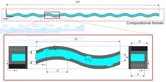
Figure 1.
Geometry of the wavy microchannel with grooves and computational domain comprising 10 cycles of wavy channel.
The information for the reference channel is shown in Table 1. In the reference channel, the horizontal locations of grooves on both the walls are the same (D = 0). Grooves are attached to crests and troughs when D = 0. As D increases, grooves on the left wall (located at z = 400 μm in Figure 1) move in the −x direction, and grooves on the right wall (located at z = 0 in Figure 1) move in the +x direction from a crest (or a trough).

Table 1.
Dimensions of the reference wavy channel with grooves.
Conjugate heat transfer analysis was carried out on the flow channel and solid domain for laminar flow in steady state using three-dimensional Navier-Stokes equations. The commercial computational fluid dynamics code ANSYS CFX 15.0® (Version 15.0, ANSYS Inc., Canonsburg, PA, USA, 2013) [] was used for the analysis. The boundary conditions are shown in Figure 2. The boundary conditions were used in the same way as in a previous study []. The working fluid was water at 300 K, and the material of the solid wall was copper.
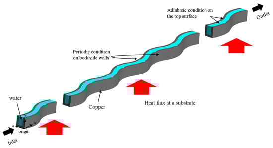
Figure 2.
Boundary conditions.
The inlet Reynolds number () was 700, and the corresponding flow rate was assigned at the inlet. The average velocity of water at the inlet is 1.992 m/s. The static pressure was used as an exit boundary condition. Periodic conditions for temperature were applied to both side boundaries (i.e., wavy surfaces) considering the neighboring microchannels. Uniform heat flux conditions (50 W/cm2) were applied to the bottom boundary (substrate), and the upper boundary was assumed to be adiabatic.
The fluid and solid computational domains consist of hexahedral and unstructured tetrahedral meshes, respectively. Since the flow velocity changes near the groove, dense meshes are placed there. Near the solid wall, dense meshes were also placed in anticipation of large temperature and velocity gradients due to the boundary layer. Figure 3 shows an example of the grid system. Convergence conditions were set so that the root-mean-squared residual values of all parameters fell to 1.00 × 10⁻⁶. Each computation took about 5–6 h on a computer with an Intel Core i7–4790K 4GHz CPU.
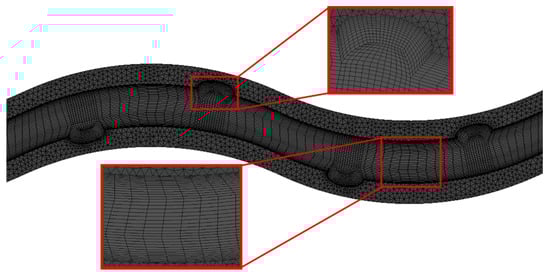
Figure 3.
Example of a computational grid system on one cycle of wavy channel.
3. Optimization Procedure
The multi-objective optimization problem was formulated as follows:
Minimize: F(x) = [F1(x), F2(x)]
Design variable bound: LB ≤ x ≤ UB, x∈R,
where F(x) is the vector of real-valued objective functions, x is a vector of the design variables, and LB and UB indicate the vectors of the lower and upper bounds, respectively []. Figure 4 shows a flowchart for the multi-objective genetic algorithm (MOGA) optimization process using a surrogate model. Firstly, the objective functions and constraints are defined according to the design goals. Secondly, the design variables and their ranges are selected.
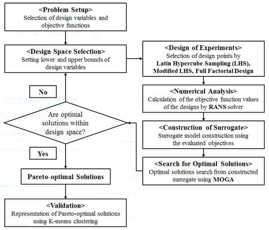
Figure 4.
Multi-objective optimization procedure.
The full factorial method, LHS, and modified LHS were used in DOE to select design points (i.e., sample designs). Values of the objective functions were evaluated by numerical analysis at these design points. Next, to approximate the objective functions, surrogate models were constructed using these objective function values. A genetic algorithm (GA) was used to find the global optima. Finally, Pareto-optimal solutions (a collection of non-dominated solutions) were derived using MATLAB (Release 14, the Math Work Inc., Natick, MA, USA, 2004) [].
3.1. Design Variables and Objective Functions
For optimization, three geometric parameters were selected as the design variables through a preliminary parametric study: the ratio of the groove depth to half of the side wall thickness (d/t), the ratio of the groove width to half of the cycle length (w/P), and the distance between staggered grooves on the opposite walls to half of the cycle length (D/P). The depth and width of the grooves were expected to affect the vortices occurring around the grooves and thus have sensitive effects on the heat transfer. The distance between staggered grooves affects the disturbance of the main flow.
The average Nusselt number is defined as follows []:
where Dh is the hydraulic diameter of the microchannel, and kw is the thermal conductivity of water. is the average convective heat transfer coefficient, which is defined as follows:
where q is the heat flux, Ab and Ac are the bottom area and the side area of the flow channel, and Tw and Tm are the average temperature at the solid wall and the average of the inlet and outlet temperatures, respectively.
The friction factor f is defined as follows []:
where dp, , and U are the pressure difference between the inlet and outlet, the density of water, and the average velocity at the inlet, respectively. The thermal resistance Rth is defined as follows []:
where Ts,max and Tf,inlet are the highest temperature at the bottom substrate and the average temperature of the cooling fluid at the inlet, respectively, and A is the area of the microchannel substrate. The local Nusselt number (Nux) is defined as follows:
where ql and Tw,l are the local heat flux and local temperature at the surface of the solid wall, respectively.
Rth and f were selected as objective functions for the multi-objective optimization: FRth = Rth and Ff = f. The thermal resistance Rth is related to the highest local temperature, which affects the performance of micro devices. The friction factor f was used to reduce the pressure drop through the microchannel. A parametric study was carried out for the performance functions using three design variables: D/P, w/P, and d/t. Based on the parametric study, the ranges of the three design variables were selected, as shown in Table 2.
Table 2.
Ranges of design variables.
3.2. Modified LHS
Factorial design [,] is a classical DOE method that explores the design space. 2–level and 3–level full factorial designs are widely used to estimate interactions between design variables. Figure 5 shows examples of 2– and 3–level full factorial designs for two design variables. In the 2–level full factorial design, the sample points are located at the ends of each boundary, as shown in Figure 5a. In the 3–level full factorial design, the sample points are located at the ends and middle of each boundary, as shown in Figure 5b. In these full factorial designs, the distribution and number of the sample points are determined according to the number of design variables when the level is determined.
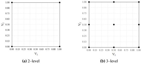
Figure 5.
Examples of the full factorial designs.
LHS [] is one of the most popular DOE methods for random sample distributions. To allocate p samples using LHS, the range of each parameter is separated into p bins, which yields a total number of pn bins for n design variables in the design space. The samples are randomly chosen in the design space, each sample is randomly arranged inside a bin, and for all one-dimensional projections of the p samples and bins, there is exactly one sample in each bin, as shown in Figure 6. Therefore, LHS is relatively incapable of handling samples at the boundaries of the design space compared to the full factorial designs.
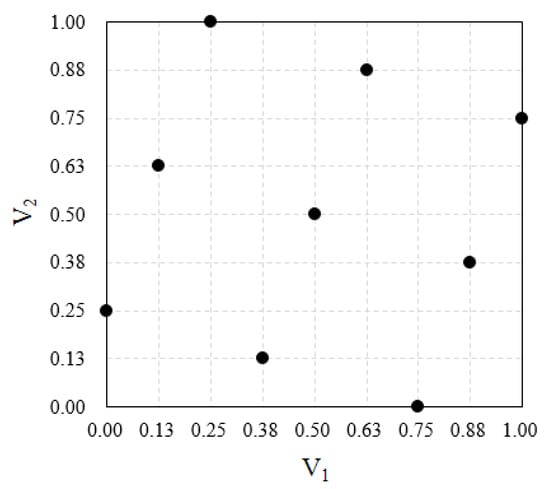
Figure 6.
Example of conventional LHS.
Since the surrogate model is built using the data at the sample points, the distribution of the sample points has a very significant influence on the prediction accuracy of the surrogate model. Therefore, when using LHS with sample points concentrated inside the design space, it is possible to predict the interaction well inside the design space, but predictions that are too high may occur at the boundaries where there are no data. On the other hand, in the full factorial design, the sample points are focused on the boundaries of the design space, so it is possible to make a relatively accurate prediction at the boundaries, but there is a problem in the prediction inside the design space.
To solve this problem, a modified LHS is proposed. In the modified LHS, sample points are extracted using the 2–level full factorial method at the boundaries of the design space, and the LHS method is used to select sample points inside the design space. An example of the modified LHS for two design variables is shown in Figure 7. In this method, the surrogate model does not show high predictions at the boundaries of the design space. Furthermore, by selecting the sample points inside the design space, the shortcomings of the full factorial design can be overcome. MATLAB [] was used to extract the sample points. Three–level full factorial design, LHS, and the modified LHS were tested for the same optimization problem. Twenty-seven sample points were extracted for all these DOE methods.
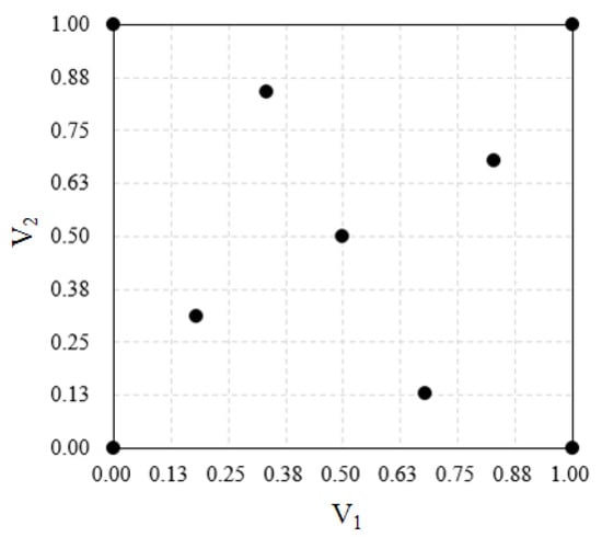
Figure 7.
Example of the modified LHS.
3.3. Surrogate Model and Searching Algorithm
The surrogate model was configured based on the sample points obtained using DOE methods. Response surface approximation (RSA) [] was used as the surrogate model. MOGA coupled with the RSA model was used to obtain Pareto-optimal solutions [].
The RSA model is multivariate polynomial model, and a continuous response y(x) is usually modeled as follows []:
where x is a vector of design variables, fj(x) (j = 1, …, N) are the terms of the model, βj (j = 1, …, N) are the coefficients, and the error ε is assumed to be uncorrelated and distributed with a mean of 0 and constant variance []. A second-order polynomial is used for the RSA model, and the model can be expressed as follows:
The model involves an intercept, linear terms, quadratic interaction terms, and squared terms (from left to right). R2 and Radj2 are used to decide the goodness of the fit and should be close to 1 for a good fit [].
GA is a random global search technique that solves problems based on natural evolution. An initial population of individuals is defined to represent a part of the solution to a problem []. Before starting the search, a set of chromosomes is randomly selected from the design space to obtain the initial population. Through subsequent computations, the individuals adapt in a competitive way. The initially selected set of chromosomes is called the parental generation, and the subsequent selected set of chromosomes is called the child generation. In this process, genetic search operators (selection, mutation, and crossover) are used to obtain chromosomes that are superior to the previous generation []. MATLAB [] was used to invoke the GA for multi-objective optimization.
4. Results and Discussion
4.1. Grid Dependency Test and Validation of Numerical Results
A grid dependency test was carried out for the reference shape based on Richardson’s extrapolation method and grid convergence index (GCI), which represents numerical uncertainty by estimating the discretization error according to the procedure presented by Roache [] and Celik and Karatekin [].
Table 3 shows the results of calculating the discretization error for . The number of grid nodes was adjusted by setting the grid segmentation index to 1.3, and three different grid systems were analyzed. When N2 was used, the extrapolation error () was about 0.3%, and was about 0.4%, which indicate small numerical uncertainty. Therefore, N2 was selected as the optimal grid system.
Table 3.
Analysis of grid convergence index.
To verify the numerical results, they were compared with experimental data obtained by Sui et al. [] for the Nusselt number and friction factor in a wavy microchannel under the same boundary conditions, as shown in Figure 8. As shown in Figure 8, the numerical results for the friction factor show good agreement with the experimental data, except at the lowest Reynolds number. The numerical results for the Nusselt number deviate slightly from the experimental data over the whole Re range but show the same qualitative tendency. At Re = 300, the errors are relatively large because the pressure drop and the flow rate are relatively small, as discussed by Sui et al. [].
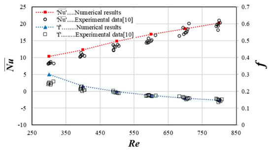
Figure 8.
Validation of numerical results compared with experimental data [].
4.2. Heat Transfer Performance Enhancement by Grooves
Table 4 shows the comparison of the performance parameters between the smooth and reference wavy microchannels. In the wavy channel with grooves, increased by about 8.34%, and Rth decreased by about 2%, but the friction factor f also increased by about 1.25% in comparison with the smooth wavy channel. This means that the grooves largely enhance the heat transfer but with less increase in the friction. This improvement in the heat sink performance with grooves is expected to be further increased by optimization.
Table 4.
Performance comparison between reference and smooth wavy microchannels.
The temperature distributions on the wavy wall on the right side of the reference and smooth microchannels are shown in Figure 9. In the case of the reference design, it can be seen that the temperature increase in the flow direction is smaller than that of the smooth microchannel, resulting in lower maximum temperature. This shows improved heat transfer performance on the sidewalls and confirms the results shown in Table 4.
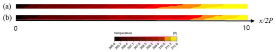
Figure 9.
Temperature distributions on a right side wall: (a) smooth microchannel and (b) reference design.
The local Nusselt number (Nux) distributions on the wavy side walls are shown in Figure 10. High Nux regions are found between the crest and the trough (e.g., x/2P = 5.75–6.25) on the left wall, but they are found between a trough and crest (e.g., x/2P = 6.25–6.75) on the right wall. In addition, most of the high Nux regions are distributed near the top and bottom of the flow path. In the case of the smooth microchannel, a low Nux region is found near the middle height of the flow path immediately after each crest (e.g., x/2P = 5.75). In the reference design, the high Nux regions are found just downstream of the grooves, and the total area of the high Nux regions is larger than that of the smooth channel. This results in high in the grooved microchannel, as shown in Table 4.
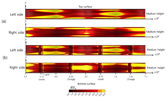
Figure 10.
Local Nusselt number distributions on wavy walls: (a) smooth microchannel and (b) reference design.
Figure 11 shows the flow fields of the reference design and the smooth wavy microchannel. Figure 11a shows that the velocity gradients near the left wall are larger than those near the right wall between a crest and trough (x/2P = 5.75–6.25), but vice versa between the trough and crest (x/2P = 6.25–6.75). This phenomenon occurs due to the fluid inertia. The regions with high velocity gradients and those with high Nux shown in Figure 10 are nearly the same. Thus, it can be inferred that the high velocity gradient near the wall promotes the heat transfer and enhances Nux.
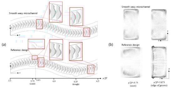
Figure 11.
Velocity vectors on x–z plane and y–z plane (a) velocity vectors on the x–z plane (y/H = 0.6) (b) velocity vectors on the y–z plane.
Figure 11b shows the velocity vectors in the y–z plane. Vortices are found near the top and bottom of the flow channel in the crest. In the case of the reference design with grooves, a complicated flow structure is found near the left wavy wall at the edge of a groove (x/2P = 5.875) due to the upward flow escaping from the groove, which promotes mixing of the fluid (and thereby heat transfer) in these regions. This is due to sudden contraction of the flow area just downstream of a groove and provides a reason for the high Nux regions downstream of the grooves shown in Figure 10b. Even though the grooves are at the same locations on both the wavy walls, the flow fields shown in Figure 11b are not symmetric in the z direction because the main flow upstream of the groove proceeds in the +z direction.
Figure 12 shows the temperature distributions in the y–z plane at the inflection point of the wavy channel (x/2P = 6). The temperature gradient is relatively small near the upper and lower sides of the flow path in common. This is thought to be due to the strong vortices shown in Figure 11b. These low temperature gradients also contribute to the distribution of high Nux in these regions (Figure 10). Figure 12 shows that the temperature on the left side in the reference design is still low, even at the medium height, unlike in the smooth wavy microchannel. This is due to the fluid mixing caused by the strong secondary flow downstream of the grooves.
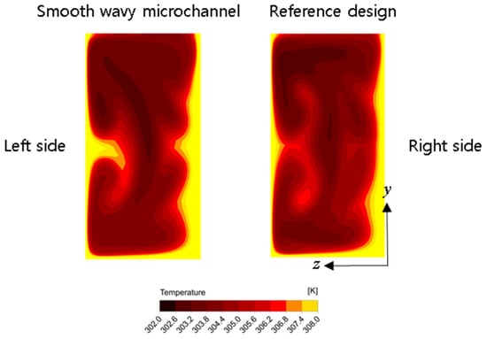
Figure 12.
Temperature distributions at inflection point (x/2P = 6) in the y–z plane.
4.3. Parametric Study
Figure 13 shows the results of the parametric study for , Rth, and f. When one parameter was changed, the other parameters were fixed at the reference values shown in Table 2. With the change of parameters, the friction factor f shows small variations of less than 2.5%. At d/t = 0.5, the maximum and f and minimum Rth are found, which indicates that there is an optimum groove depth for heat transfer enhancement.
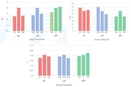
Figure 13.
Results of the parametric study.
Rth and are inversely correlated with the variation of d/t. and f have maximum values at w/P = 0.15, but Rth has a minimum value at w/P = 0.25. Rth decreases as w/P increases in the tested range. This means that wide grooves are effective in reducing thermal resistance. In the case of D/P, and f increase as D/P increases, but Rth shows a maximum at D/P = 0 (non-staggered grooves). This indicates that if the absolute value of D is fixed, the relative locations of grooves between the two wavy walls do not affect Rth unlike and f.
At D/P = 0.5, shows the maximum value of 20.2. This is the value improved by 23.2% from the value () of the wavy microchannel heat sink without grooves predicted by Sui et al. [] under the same geometric and Reynolds number conditions.
4.4. Optimization Results with Different DOEs
Figure 14 shows the distribution of sample points of three different DOEs. In Figure 14a, the 3-level full factorial design shows that the sample points are located on only the boundaries of the design space. In the case of the conventional LHS, the sample points are distributed in only the design space, as shown in Figure 14b. However, in the modified LHS, the sample points are located on the boundaries and inside of the design space, as shown in Figure 14c. The RSA models for the objective functions, Ff and FRth, were formulated in terms of the design variables normalized between 0 and 1 for three different DOEs as follows:
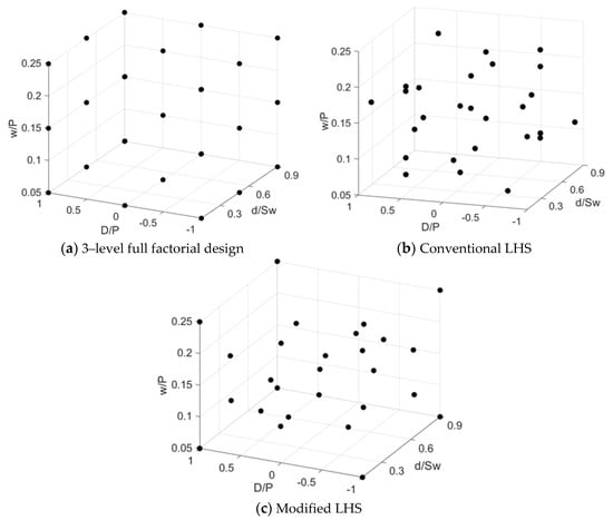
Figure 14.
Distributions of sample points for three different DOEs.
Figure 15 shows the Pareto-optimal solutions using three different DOEs. The Pareto-optimal solutions are the best solutions that can be achieved for one objective without disadvantaging another objective and are sensitive to the constructed surrogate model []. Pareto-optimal fronts obtained using the conventional and modified LHS methods have similar smooth curves, as shown in Figure 15. However, the full factorial design shows a curve that has two inflection points, unlike the other curves. The Pareto-optimal front from modified LHS predicts the lowest optimum values of the two objective functions among the tested DOEs in most of the range. The Pareto-optimal fronts of the two LHS methods cover wider ranges than that of the full factorial design.
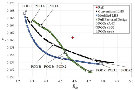
Figure 15.
Pareto-optimal solutions for three different DOEs.
To compare the optimization results, three Pareto-optimal designs (PODs) were extracted from each Pareto-optimal front using K-means clustering [], as presented in Figure 15. The predicted objective function values at the PODs and numerical calculations at the same PODs are compared in Table 5. In case of the full factorial design, the PODs are close to the boundaries of one or two design variables. However, the PODs of conventional LHS are found inside the design space. In this case, a POD close to a boundary (D/P = −0.8802 in POD A) yields a larger relative error between the predicted and calculated objective function values than the other PODs. As mentioned earlier, the surrogate model obtained using conventional LHS over-predicts the values at the boundary of the design space, and the error increases near the boundary.
In the case of the modified LHS, even the POD located close to the boundary shows good prediction with maximum relative error less than 1.5%. Thus, the modified LHS shows the best prediction accuracy among the tested DOEs. The full factorial design and conventional LHS generally over-predict the objective function values with positive relative errors at the three PODs, but the modified LHS generally under-predicts the values. Therefore, there is not much difference in the calculated objective function values at the PODs among the tested DOEs.
The R2 and adjusted R2 values of the RSA models constructed using three different DOEs are listed in Table 6. As mentioned earlier, values closer to 1 indicate a better surrogate model. In this respect, the modified LHS shows the best results in Table 6. This is consistent with the results shown in Table 5. In addition, the RSA model with the full factorial design has the worst performance. Applying a DOE method that properly locates the sample points on the boundaries and inside of the design space makes it possible to construct a more accurate surrogate model and obtain superior optimization results.
4.5. Analysis of the Optimized Design
POD 2 obtained with the modified LHS was selected for further analysis because the values of both the objective functions were improved compared to the reference design. In POD 2, Rth and f are reduced by 1.55% and 3.00%, respectively, compared with those of the reference design. The Nux distributions on the wavy walls are shown in Figure 16, which compares the heat transfer performance between POD 2 and the reference design. In the case of the reference design, there are high Nux regions on the left wall between the grooves in the crest and the trough (x/2P = 5.75–6.25). In the case of POD 2, high Nux regions are shown on the left side wall between the inflection point where the groove is located and the trough (x/2P = 5.50–6.25). The right wall between x/2P = 7.00 and 7.50 shows the same Nux distribution as the left wall between x/2P = 5.50 and 6.25. Unlike the reference design, the high Nux distribution for POD 2 from the inflection point to the crest (x/2P = 5.50–5.75) seems to be one of the important factors in reducing Rth compared to the reference design.
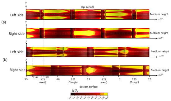
Figure 16.
Local Nusselt number distributions on wavy walls: (a) reference design, and (b) optimal design (POD2).
Figure 17 shows the streamlines and velocity vectors. Figure 17a shows that the recirculating flow develops in the grooves in the reference design. These recirculating flow regions correspond to the low Nux regions in the grooves in Figure 16. This occurs because the flow recirculation hinders the heat transfer on the wall. Figure 17b shows the velocity vectors at the cross sections perpendicular to the flow direction. As mentioned earlier, in the reference design, a strong interaction between the vortical flow in the channel and upward flow from the groove is found near the left wall at the edge of the groove (x/2P = 5.875). In the case of POD 2, this phenomenon is also found near the left wavy wall at the edge of the groove (x/2P = 5.593) but is weaker than in the reference design. This seems to be affected by the location of the groove (which is the crest in the reference design but an inflection point in POD 2) and the fact that the two grooves on both the walls are attached at the same location in the reference design.
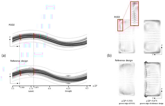
Figure 17.
Streamlines and velocity vectors: (a) streamline distributions on the x–z plane (y/H = 0.6) (b) velocity vector in cross-section perpendicular to flow direction.
However, in POD 2, the vortices in the channel become stronger at a location downstream (x/2P = 5.875). This is consistent with the Nux distributions shown in Figure 16. In the reference design, the high Nux region persists from the groove edge (x/2P = 5.875) to a location far downstream but disappears before the next groove. However, in POD 2, the high Nux region is relatively narrow at the edge of the groove (x/2P = 5.593) but grows downstream and becomes widest at the upstream edge of the next groove. Thus, the total area of the high Nux regions is larger in POD 2 than that in the reference design.
5. Conclusions
A wavy microchannel heat sink with grooves was optimized using RANS analysis of the flow and conjugate heat transfer. In the reference wavy channel with grooves, increased by about 8.34%, and Rth decreased by about 2%, but the friction factor f also increased by about 1.25% compared to the smooth wavy channel. Thus, using grooves, the enhancement of the heat transfer surpasses the increase in the friction.
For optimization, the distance between staggered grooves on opposite wavy walls, the groove depth, and the groove width were selected as design variables. The thermal resistance (Rth) and friction factor (f) were used as objective functions. A modified LHS that uses the advantages of conventional LHS and the three–level full factorial method was also proposed. The optimization performance of three DOE methods was estimated. Surrogate models of the objective functions were constructed by RSA with each DOE method. The corresponding Pareto optimal solutions were derived, and three representative optimal solutions were selected to compare the predictions of the DOE methods.
The results showed that the optimal solutions using modified LHS methods have the best predictions with less than 1.5% error compared to the numerical calculations. They also had the largest R2 and adjusted R2 values, which indicate the best statistical accuracy of the RSA models. For one of the representative optimal solutions, POD2, Rth and f decreased by 1.55% and 3.00%, respectively, compared to the reference design, indicating that both the objective functions were improved. Therefore, the multi–objective optimization with modified LHS could effectively improve the performance of the wavy microchannel heat sink with grooves.
Author Contributions
M.-C.P. presented the main idea of the wavy microchannel heat sink with groove; M.-C.P. and S.-B.M. contributed to the overall composition and writing of the manuscript; M.-C.P. analyzed the proposed wavy microchannel with grooves and performed the numerical analysis; S.-B.M. analyzed the data; K.-Y.K. revised and finalized the manuscript. All authors have read and agreed to the published version of the manuscript.
Funding
This work was supported by the National Research Foundation of Korea (NRF) grant funded by the Korean government (MSIT) (No. 2019R1A2C1007657).
Institutional Review Board Statement
Not applicable.
Informed Consent Statement
Not applicable.
Data Availability Statement
Data is contained within the article.
Conflicts of Interest
The authors declare no conflict of interest.
Nomenclature
| Ab | The bottom area of the flow channel (m2) |
| As | Side area of the flow channel (m2) |
| d | Groove depth (μm) |
| D | Distance between staggered grooves (μm) |
| Dh | Hydraulic diameter (m) |
| F | Friction factor |
| h | Height of flow path (μm) |
| H | Height of microchannel (μm) |
| kw | Thermal conductivity (W/K) |
| Nu | Nusselt number |
| Nux | Local Nusselt number |
| U | Average velocity at the inlet (m/s) |
| p | Pressure (N/m2) |
| P | Half of wave length of channel wall (μm) |
| q | Heat flux (W/cm2) |
| Re | Reynolds number |
| Rth | Thermal resistance (K/W) |
| t | Side wall thickness of channel (μm) |
| Tw | Average temperature at the solid wall (K) |
| Tm | Average temperature of the inlet and outlet (K) |
| Ts,max | Highest temperature at the bottom substrate (K) |
| Tf,inlet | Average temperature of the cooling fluid at the inlet (K) |
| w | Groove width (μm) |
| W | Width of channel (μm) |
| x, y, z | Rectangular coordinates |
| ρ | Density (kg/m3) |
References
- Sauciuc, L.; Chrysler, G.; Mahajan, R.; Szleper, M. Air-cooling Extension-Performance Limits for Processor cooling applicatioins. In Proceedings of the 19th Annual IEEE Semiconductor Thermal Measurement and Management Symposium, San Jose, CA, USA, 11–13 March 2003; pp. 74–81. [Google Scholar]
- Krishnan, S.; Garimella, S.V.; Chrysler, G.M.; Mahajan, R.V. Towards a Thermal Moore’s Law. IEEE Trans. Adv. Packag. 2007, 30, 462–474. [Google Scholar] [CrossRef]
- Tuckerman, D.F.; Pease, R.F.W. High-Performance heat sinking for VLSI. IEEE Electron Device Lett. 1981, 2, 126–129. [Google Scholar] [CrossRef]
- Wang, G.-L.; Yang, D.-W.; Wang, Y.; Niu, D.; Zhao, X.-L.; Ding, G.-F. Heat Transfer and Friction Characteristics of the Microfluidic Heat Sink with Variously-Shaped Ribs for Chip Cooling. Sensors 2015, 15, 9547–9562. [Google Scholar] [CrossRef] [PubMed]
- Ansari, D.; Husain, A.; Kim, K.-Y. Multiobjective Optimization of a Grooved Micro-Channel Heat Sink. IEEE Trans. Components Packag. Technol. 2010, 33, 767–776. [Google Scholar] [CrossRef]
- Farhanieh, B.; Herman, C.; Sundén, B. Numerical and experimental analysis of laminar fluid flow and forced convection heat transfer in a grooved duct. Int. J. Heat Mass Transf. 1993, 36, 1609–1617. [Google Scholar] [CrossRef]
- Greiner, M.; Spencer, G.J.; Fischer, P.F. Direct Numerical Simulation of Three-Dimensional Flow and Augmented Heat Transfer in a Grooved Channel. J. Heat Transf. 1998, 120, 717–723. [Google Scholar] [CrossRef]
- Xie, Y.; Shen, Z.; Zhang, D.; Lan, J. Thermal Performance of a Water-Cooled Microchannel Heat Sink With Grooves and Obstacles. J. Electron. Packag. 2014, 136, 021001. [Google Scholar] [CrossRef]
- Gong, L.; Kota, K.; Tao, W.; Joshi, Y. Parametric Numerical Study of Flow and Heat Transfer in Microchannels with Wavy Walls. ASME J. Heat Transf. 2011, 133, 1356–1373. [Google Scholar] [CrossRef]
- Sui, Y.; Lee, P.; Teo, C. An experimental study of flow friction and heat transfer in wavy microchannels with rectangular cross section. Int. J. Therm. Sci. 2011, 50, 2473–2482. [Google Scholar] [CrossRef]
- Qun, A.K.; Huang, V.L.; Suganthan, P.N. Differential Evolution Algorithm with Strategy Adaption for Global Numerical Optimization. IEEE Trans. Evol. Comput. 2008, 13, 398–417. [Google Scholar] [CrossRef]
- Leung, Y.W.; Wang, Y. An orthogonal genetic algorithm with quantization for global numerical optimization. IEEE Trans. Evol. Comput. 2001, 5, 41–53. [Google Scholar] [CrossRef]
- Tu, Z.; Lu, Y. A robust stochastic genetic algorithm (StGA) for global numerical optimization. IEEE Trans. Evol. Comput. 2004, 8, 456–470. [Google Scholar] [CrossRef]
- Kim, J.-H.; Ovgor, B.; Cha, K.-H.; Kim, J.-H.; Lee, S.; Kim, K.-Y. Optimization of the Aerodynamic and Aeroacoustic Performance of an Axial-Flow Fan. AIAA J. 2014, 52, 2032–2044. [Google Scholar] [CrossRef]
- Kim, K.-Y.; Samad, A.; Benini, E. Design Optimization of Fluid Machinery; John Wiley & Sons. Ltd.: Hoboken, NJ, USA, 2019; ISBN 978-1-119-18829-2. [Google Scholar]
- Robinson, T.D.; Eldred, M.S.; Willcox, K.E.; Haimes, R. Surrogate-Based Optimization Using Multifidelity Models with Variable Parameterization and Corrected Space Mapping. AIAA J. 2008, 46, 2814–2822. [Google Scholar] [CrossRef]
- Regis, R.G. Trust regions in Kriging-based optimization with expected improvement. Eng. Optim. 2016, 48, 1037–1059. [Google Scholar] [CrossRef]
- Buragohain, M.; Mahanta, C. A novel approach for ANFIS modelling based on full factorial design. Appl. Soft Comput. 2008, 8, 609–625. [Google Scholar] [CrossRef]
- Pholdee, N.; Bureerat, S. An efficient optimum Latin hypercube sampling technique based on sequencing optimization using simulated annealing. Int. J. Syst. Sci. 2013, 46, 1780–1789. [Google Scholar] [CrossRef]
- Goel, T.; Haftka, R.T.; Shyy, W.; Queipo, N.V. Ensemble of surrogates. Struct. Multidiscip. Optim. 2006, 33, 199–216. [Google Scholar] [CrossRef]
- Deb, K.; Agrawal, S.; Pratap, A.; Meyarivan, T. A Fast Elitist Non-Dominated Sorting Genetic Algorithm for Multi-Objective Optimization: NSGA-II. In Parallel Problem Solving from Nature PPSN VI; Springer: Berlin/Heidelberg, Germany, 2000; pp. 849–858. [Google Scholar]
- ANSYSCFX 15.0 Solver Theory Guide; ANSYS Inc.: Canonsburg, PA, USA, 2013.
- Afzal, A.; Kim, K.-Y. Optimization of pulsatile flow and geometry of a convergent–divergent micromixer. Chem. Eng. J. 2015, 281, 134–143. [Google Scholar] [CrossRef]
- MATLAB. The Language of Technical Computing; Release 14; the Math Work Inc.: Natick, MA, USA, 2004. [Google Scholar]
- Koziel, S.; Yang, X.-S. Surrogate-Based Methods. In Computational Optimization, Methods and Algorithms; Springer: Berlin/Heidelberg, Germany, 2011; Volume 356, pp. 33–59. [Google Scholar]
- Roache, P.J. Verification of Codes and Calculations. AIAA J. 1998, 36, 696–702. [Google Scholar] [CrossRef]
- Celik, I.; Karatekin, O. Numerical Experiments on Application of Richardson Extrapolation with Nonuniform Grids. J. Fluids Eng. 1997, 119, 584–590. [Google Scholar] [CrossRef]
- Baumgartner, U.; Magele, C.; Renhart, W. Pareto Optimality and Particle Swarm Optimization. IEEE Trans. Magn. 2004, 40, 1172–1175. [Google Scholar] [CrossRef]
- Afzal, A.; Kim, K.-Y. Three-objective optimization of a staggered herringbone micromixer. Sens. Actuators B Chem. 2014, 192, 350–360. [Google Scholar] [CrossRef]
Publisher’s Note: MDPI stays neutral with regard to jurisdictional claims in published maps and institutional affiliations. |
© 2021 by the authors. Licensee MDPI, Basel, Switzerland. This article is an open access article distributed under the terms and conditions of the Creative Commons Attribution (CC BY) license (http://creativecommons.org/licenses/by/4.0/).