Numerical Analysis of a Flow over Spheres Embedded on a Flat Wall

Abstract

This paper presents the results of numerical simulations of flow in a periodic channel with the walls covered in the central part by spherical elements that have the same overall surface areas but different radii. Two distributions of the sphere are considered, with the subsequent rows placed one after another or shifted. The computations are performed using the high-order code, whereas the solid elements are modelled with the help of the immersed boundary method. For selected cases, the results are validated by comparison with the solutions obtained using the ANSYS Fluent code on a very dense body-fitted mesh. It was found that the increase in the sphere diameter slows down the flow, which is attributed to the larger blockage of the channel cross-section caused by larger spheres and the occurrence of intense mixing (recirculation) between the spheres. The velocity profiles in the vicinity of the sphere are largely dependent on sphere diameter and rise when it increases. It was found that the distribution of the spheres plays an important role only when the spheres are large. In the part of the channel far from the sphere, the velocity profiles are significantly influenced by the sphere diameter but seem to be independent of the sphere distributions.

1. Introduction

Flows over rough surfaces occur commonly in nature and the industry. Roughness is often the result of natural processes based on adaptation to environmental conditions (e.g., tree bark or animal skin) or created purposely to improve or control the efficiency of technical devices (e.g., heat exchangers, golf balls, turbine blades, airplanes). In the latter case, the required roughness is usually obtained during the manufacturing process by shaping the walls to obtain waviness or by embedding small solid elements on their surfaces. The type of roughness is particularly important when the roughness height is large compared to the boundary layer thickness and changes not only the near-wall flow characteristics but also affects the mean flow quantities. This often happens in microchannels, where even small changes in wall topology can significantly impact local and global flow behavior (e.g., laminar-turbulent transition, drag force). Experimental analysis of the flow over rough walls is possible but cumbersome as it requires very precise placing of measurement probes (thermocouples, pressure probes, laser beam cross-section) in between particular surface elements or waviness. Often, the impact of wall topology is analyzed from the point of view of its influence on the flow parameters downstream of the rough wall. For example, Dróżdż et al. [1] analyzed the effect of amplitude waviness on the skin friction and separation behind the wavy wall part.

The rapid development of computers and novel computational methods allows for the investigation of the flows over the rough walls using computational fluid dynamics (CFD) that employs direct numerical simulation (DNS) or large eddy simulation (LES). Chan et al. [2] investigated the flow in a pipe with a sinusoidal wall. They found that the inclination of waviness is as important as its height. Flows over sinusoidal walls of various frequencies and amplitudes were analyzed by, among others, Dharaiya and Kandlikar [3], Cherukat et al. [4], Kaisar et al. [5], Bhaganagar et al. [6] and Harikrishan et al. [7]. They found that the waviness of the wall increases velocity fluctuations and vorticity magnitude, which in non-isothermal problems, intensifies the heat transfer between the flowing medium and the wall. Harikrishan et al. [7] analyzed the impact of wall skewness on flow and heat transfer. It was reported that the skewness induces secondary flows, which increases the overall tridimensionality of the flow that enhances the heat exchange. Hu et al. [8], Croce and D’Agaro [9], and Guo et al. [10] considered the roughness formed by rectangular, triangular, prismatic elements or peaks distributed randomly or in a predefined manner. They found that the topology of these elements, both the type and localization, significantly affects the pressure drop, drag force, and heat transfer. The impact of trapezoidal, triangular, rectangular, and cylindrical elements embedded in the walls and wall waviness on skin friction, slip velocity, and heat transfer was analyzed by Rawool et al. [11], Herwig et al. [12] and Noorian et al. [13]. A detailed analysis of flow around conical elements with various shapes placed on the walls of microchannels was performed by Croce et al. [14]. The influence of the Reynolds number and the roughness type (triangular, rectangular, spherical elements) on the Nusselt and Poiseuille number was studied by Zhang et al. [15]. They found that the type of elements affects them more than the changes in mean flow velocity.

The above brief review shows that the flows over rough walls constitute an important field of research. The variety of wall topologies and elements used to obtain roughness indicates that no definite conclusions on their optimal shapes have been formulated so far. In the present paper, we focus on the impact of half-spherical elements embedded in the wall surface on mean velocity field and its fluctuations. Rather than trying to find an optimal configuration of the sphere that would fulfil the assumed goal, we analyze whether and to what extent the size and distribution of the spheres can be treated as the parameters that control the mean flow quantities, the turbulence intensity and the mixing process. The research is performed using a high-order numerical code based on the compact difference discretization method. The solid walls together with the embedded spheres are modelled using the immersed boundary (IB) approach, which was found to be very efficient and accurate in this type of research [16,17]. In the present work, the accuracy of the IB method is confirmed by comparison with the results obtained on a body-fitted mesh.

2. Mathematical Modelling

We consider incompressible flows described by the continuity equation and the Navier–Stokes equations defined as follows:

$${\partial }_t\rho +\nabla ·\left(\rho \mathbf{u}\right)=0$$

(1)

$$\rho \left({\partial }_t\mathbf{u}+(\mathbf{u}·\nabla )\mathbf{u}\right)+\nabla p=\nabla ·\tau +{\mathbf{f}}^{\mathrm{BF}}+{\mathbf{f}}^{\mathrm{IB}}$$

(2)

where p is the hydrodynamic pressure; $\mathbf{u}$—velocity vector; $\rho$—density; $\tau$—viscous stress tensor. The term ${\mathbf{f}}^{\mathrm{BF}}$ is the source term that causes the fluid movement and ${\mathbf{f}}^{\mathrm{IB}}$ originates from the IB method. Its role is to act on the flow field as if there was a solid body embedded in the flow domain. Definitions and discussion of these terms are presented later.

2.1. Solution Algorithm

The solution algorithm for Equations (1) and (2) is formulated in the framework of a projection method for pressure-velocity coupling [18]. Time integration is based on a predictor-corrector approach (Adams–Bashforth/Adams Moulton) and the spatial discretisation is performed using the sixth-order compact difference schemes on half-staggered meshes [19,20]. Details of the IB method can be found in [21] and here, we only present its most important elements. The main solution algorithm is defined as follows.

Predictor step. Generally, we assume that the time-step ($\Delta t$) can vary as the flow velocity changes in the successive time-steps, $...,n-1,n,n+1,...$. With this assumption, the second-order Adams–Bashforth method is given as follows:

$$\begin{array}{c}\hfill \frac{\rho {\mathit{u}}^{*}-\rho {\mathbf{u}}^n}{\Delta t^n}=\left(1+\frac{\Delta t^n}{2\Delta t^{n-1}}\right)\mathrm{Res}\left({\mathbf{u}}^n\right)-\frac{\Delta t^n}{2{\Delta }^{n-1}}\mathrm{Res}\left({\mathbf{u}}^{n-1}\right)-\nabla p^n+{\mathbf{f}}^{\mathrm{BF}}+{\mathbf{f}}^{\mathrm{IB},*}\end{array}$$

(3)

where $\mathrm{Res}\left(\mathit{u}\right)$ represent the convection and diffusion terms of the Navier–Stokes equations. The source term ${\mathbf{f}}^{\mathrm{IB}}$ is integrated in time in a fully implicit manner that is discussed later. The velocity field ${\mathit{u}}^{*}$ computed from Equation (3) does not fulfil the continuity equation (i.e., ${\partial }_t\rho +\nabla ·\left(\rho {\mathit{u}}^{*}\right)\ne 0$) and according to the projection method, it must be corrected [18] using the gradients of pressure correction ($p^{\prime }$) according to the following formula:

$$\rho {\mathit{u}}^{**}=\rho {\mathit{u}}^{*}-\Delta t^n\nabla p^{\prime }$$

(4)

where $p^{\prime }$ is computed from the Poisson equation:

$$\nabla ·(\nabla p^{\prime })=\frac{1}{\Delta t^n}\left[\nabla ·\left(\rho {\mathit{u}}^{*}\right)\right]$$

(5)

resulting from the condition ${\partial }_t\rho +\nabla ·\left(\rho {\mathit{u}}^{**}\right)=0$.

Corrector step. The second-order Adams–Moulton method is defined as follows:

$$\frac{\rho {\mathbf{u}}^{*}-\rho {\mathbf{u}}^n}{\Delta t^n}=\frac{1}{2}(\mathrm{Res}\left({\mathbf{u}}^{**}\right)+\mathrm{Res}\left({\mathbf{u}}^n\right))-\nabla p^n+{\mathbf{f}}^{\mathrm{BF}}+{\mathbf{f}}^{\mathrm{IB},*}$$

(6)

Again, the velocity field ${\mathbf{u}}^{*}$ does not fulfil the continuity equation and its correction is defined as follows:

$$\rho {\mathbf{u}}^{n+1}=\rho {\mathbf{u}}^{*}-\Delta t^n\nabla p^{\prime }$$

(7)

The equation ${\rho }_t^{n+1}+\nabla ·\left(\rho {\mathbf{u}}^{n+1}\right)=0$ leads to the Poisson equation analogous to Equation (5). Its solution allows us to correct the velocity using (7) and to update the pressure field as follows:

$$p^{n+1}=p^n+p^{\prime }$$

(8)

IB–VP source term. The IB–VP method works through penalising the difference between the actual and assumed velocity of the solid body. The role of the source term ${\mathbf{f}}^{\mathrm{IB}}$ is to mimic the presence of solid objects in the flow domain. In the volume penalisation (VP) variant of the IB method, it is defined as follows:

$${\mathbf{f}}^{\mathrm{IB}}=-\frac{\rho }{\eta }\mathrm{\Gamma }\left(\mathbf{x}\right)(\mathbf{u}-{\mathbf{u}}_s)$$

(9)

where $\eta \ll 1$ is the so-called penalisation parameter measured in time units, and $\mathrm{\Gamma }$ is a phase indicator defined as follows:

$$\mathrm{\Gamma }\left(\mathbf{x}\right)=\left\{\begin{array}{cc}0,\hfill & \mathrm{for}\mathbf{x}\in {\mathrm{\Omega }}_f\hfill \\ 1,\hfill & \mathrm{for}\mathbf{x}\in {\mathrm{\Omega }}_s\hfill \end{array}\right.$$

(10)

where ${\mathrm{\Omega }}_f$ and ${\mathrm{\Omega }}_s$ represent the fluid and soild parts, respectively, of the computational domain. For $\mathrm{\Gamma }\left(\mathbf{x}\right)=1$ with $\eta \ll 1$, both Equations (3) and (6) reduce to ${\mathbf{u}}^{*}={\mathbf{u}}^{n+1}\approx \Delta t^n{\mathbf{u}}_s/(\eta +\Delta t^n)$, which for $\eta \ll \Delta t^n$ leads to ${\mathbf{u}}^{*}={\mathbf{u}}^{n+1}\approx {\mathbf{u}}_s$. Thus, the forcing term can enforce the no-slip boundary conditions on the wall or set the required velocity if the solid objects are moving. In the computations, we set $\eta ={10}^{-10}$ and the time-step computed based on the CFL criterion ($\mathrm{CFL}=0.4$) oscillated around $\Delta t=1.5\times {10}^{-4}$. The simplicity of the IB–VP method has the direct consequence of lower accuracy. Similarly, as in the classical IB method with the stepwise approach (i.e., without interpolation [22]), the formal order of the IB–VP method is at most equal to one [23,24]. However, as shown in [25], the combination of the high-order discretisation method with the IB method with the stepwise approach can lead to the solutions characterized by the second-order accuracy. We will compare the results of the IB–VP method with those obtained on a body-fitted mesh.

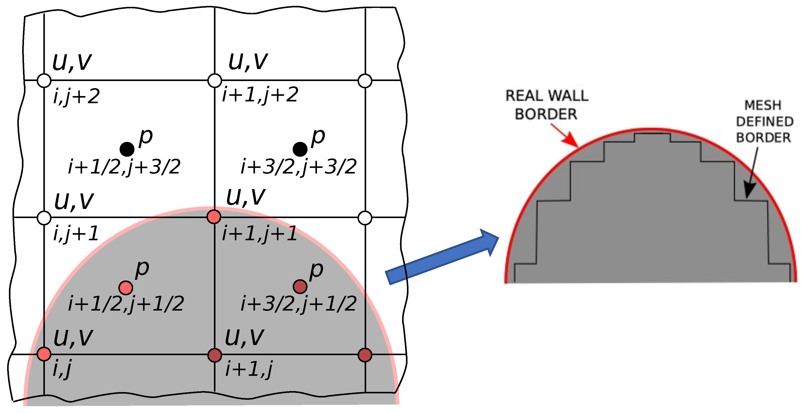
2.2. Spatial Discretisation

All terms in the continuity and the Navier–Stokes equations are discretised using a high-order compact difference method up to the sixth order. The solution algorithm is based on a half-staggered mesh in which the so-called pressure nodes are shifted to the cell centres, as shown in Figure 1. It may happen that within one computational cell, let us say ($i+3/2,j+1/2$), part of the nodes (i.e., the pressure node and three velocity nodes) lie inside the solid object, while one node ($i+2,j+1$) lies in the fluid zone. The proposed algorithm is not sensitive to these situations and such partially divided cells are treated in the same way as the cells placed fully inside or outside solid regions.

A study by [19] showed that the use of the half-staggered mesh structure has a stabilising effect, which is extremely important when high-order discretisation methods are applied. It often turns out that small discontinuities in the flow field or occurrence of large gradients of the flow variables cause instability and divergence of solution procedures [26]. Taking into account that the presence of solid elements inside the computational domains can lead to local flow discontinuities, the stabilising properties of node staggering seem to be very desirable. Indeed, the presented results show that in all analysed cases, the flow fields are smooth and free from any unwanted numerical artefacts. Details of the solution method for the algorithm not involving the IB–VP technique can be found in [19,20].

3. Computational Configuration

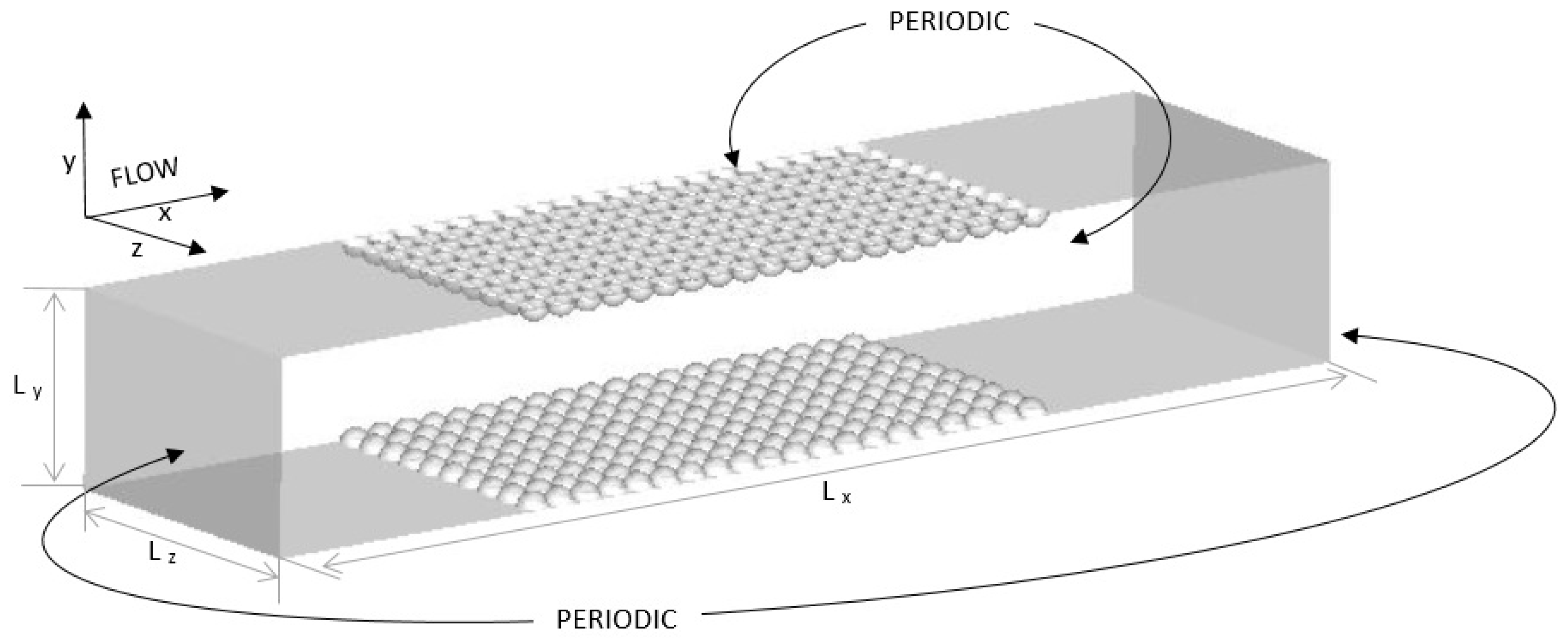
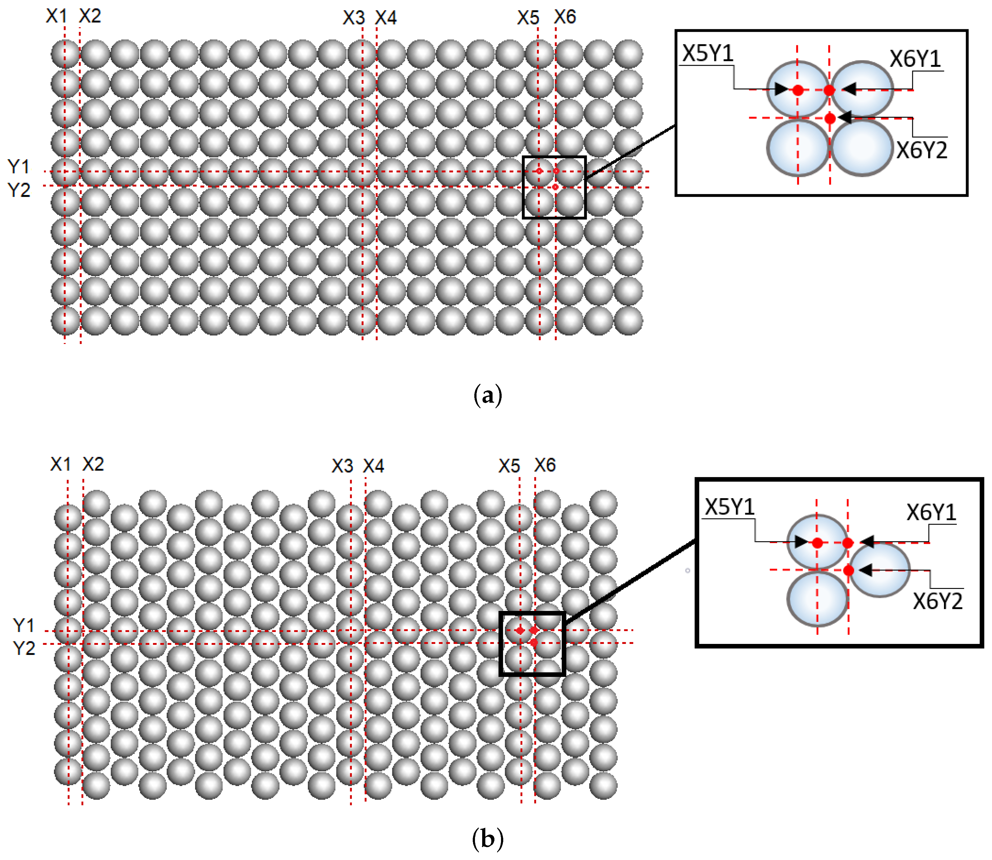
3.1. Computational Domain and Spheres Localizations

In real situations, roughness is mostly a complex 3D structure formed during the manufacturing process or created artificially by a special forming of the wall surface. In the present work, we consider the latter approach and analyse the flow in between the walls with spherical elements embedded in their surfaces. As shown in Figure 2, the spherical elements are pressed into the solid slabs to half of their diameters. The computational domain is a straight channel with dimensions $L_x\times L_y\times L_z=4\pi \times 2\times \pi$. Note that we consider a non-dimensional reference frame and refer to the Reynolds number ${\mathrm{Re}}_{\tau }=u_{\tau }h/\nu =180$, where $u_{\tau }=\sqrt{{\nu \partial u/\partial y|}_{y=\pm h}}$ is the friction velocity where u is the velocity component in the ‘x’-direction, $\nu$ is the kinematic viscosity, and $h=L_y/2$. As will be presented later, the small value of the Reynolds number allowed us to obtain accurate results without using a turbulence model. For a flat-channel configuration, the applied high-order discretisation method ensures accurate solutions on a moderate mesh density even for ${\mathrm{Re}}_{\tau }=590$, as demonstrated in [19].

The flow is periodic in the ‘x’- and ‘z’-directions and is forced by the constant pressure gradient $dp/dx=-u_{\tau }^2\rho /h$. The first row of spheres is placed at $x=\pi$, whereas the localization of the last row depends on the size of the spheres. We compare the results for three configurations in which the overall surface of all spheres is the same and equal to $S=2\times {\pi }^3$. In the first configuration, the basic one, (S1.0) there are 200 spheres with the diameter $D=\pi /10$ arranged in $10\times 20$ rows. In the configuration S0.5, there are 800 spheres ($20\times 40$ rows) with $D=\pi /20$, whereas in the configuration S2.0, there are 50 spheres with $D=\pi /5$ in $5\times 10$ rows. Note that the cross-sectional areas of the spheres in particular configurations are equal to $\mathrm{\Omega }=10\times \pi D^2/4=10\times \pi {(\pi /10)}^2/4={\pi }^3/40$ (in the configuration S1.0), $\mathrm{\Omega }=20\times \pi {(\pi /20)}^2/4={\pi }^3/80$ (in S0.5), and $\mathrm{\Omega }=5\times \pi {(\pi /5)}^2/4={\pi }^3/20$ (in S2.0), which means that the largest blockage of the channel ($B=\mathrm{\Omega }/(L_z\times L_y)$) occurs in the case S2.0 and it equals to $B={\pi }^2/40$. It is two times larger than in S1.0 ($B={\pi }^2/80$) and four times than in S0.5 ($B={\pi }^2/160$).

We analyse how the sphere size affects the mean flow velocity and fluctuations. Furthermore, we verify to what extent the ordering of the spheres in subsequent rows influences the velocity field. We consider two sphere arrangements presented in Figure 3. In the first one, the spheres are orderly placed one after another. In the second case, the subsequent rows are shifted in the ‘z’-direction by the half diameter. Note that in the former situation, the spheres are in contact along the ‘x’- and ‘z’-directions. In the latter, the spheres touch one another only along the ‘z’-direction, whereas in the ‘x’-direction, there are small gaps between them. In the following analyses, these configurations are denoted by the letter ‘o’ or ‘s’ added to the case name, e.g., S1.0o, S1.0s, S2.0o, etc. At this point, one should mention that an alternative approach to the constant overall spheres surface would be to assume the same volume of spheres. However, the present settings seem to be more meaningful for the heat transfer processes, which directly depend on the surface area being in contact with a flowing medium.

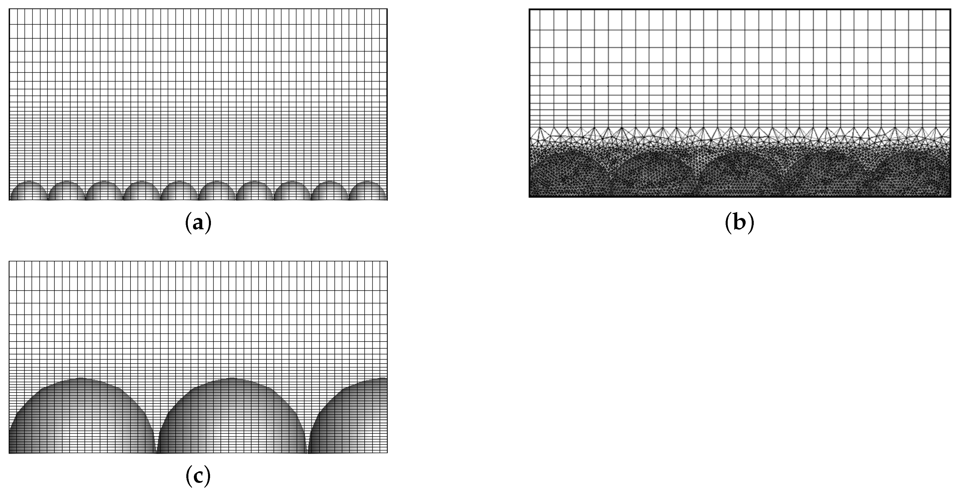
3.2. Computational Meshes

The computations were performed for two computational meshes consisting of $400\times 96\times 100$ and $600\times 144\times 150$ nodes in the ‘x’-, ‘y’- and ‘z’-directions, respectively. In both cases, the meshes were uniform in the ‘x’- and ‘z’-directions and compacted towards the walls up to the region slightly above the largest sphere, as can be seen in Figure 4a,c showing the coarse mesh and the spheres in the configurations S0.5 and S2.0 visible in the background. In the vicinity of the spheres and flat walls, the cell sizes in the ‘y’-direction were uniform and set such that $y+=u_{\tau }\Delta y/\nu$ in the near-wall point was equal to $y+=2.05$ (coarse mesh), and $y+=0.995$ (dense mesh). Note, that depending on the sphere sizes, their volumes were discretised by different numbers of mesh points.

Table 1. Characteristics of the computational meshes.

	S0.5			S1.0			S2.0
Mesh	D/Δx	D/Δy	D/Δz	D/Δx	D/Δy	D/Δz	D/Δx	D/Δy	D/Δz
Coarse	5.0	13.81	5.0	10.0	27.63	10.0	20.0	55.26	20.0
Dense	7.5	28.11	7.5	15.0	56.22	15.0	30.0	112.44	30.0

shows the ratios of the sphere diameters to the cell sizes $\Delta x$, $\Delta y$ and $\Delta z$ on the coarse and dense mesh. It can be seen that in the ‘y’-direction, there are significantly more points across the spheres than in the ‘x’- and ‘z’-directions. The preliminary computations with different mesh densities have shown that the mesh resolution in the ‘y’-direction is crucial for obtaining accurate results. The test simulations performed with the help of the ANSYS Fluent code were performed for the configuration S1.0. In this case, the mesh was fitted to the sphere surfaces, as shown in Figure 4b, and consisted of $17.5\times {16}^6$ cells compacted towards the wall such that $y+<1.0$ both on the flat channel parts and on sphere surfaces. These computations were carried out using the LES method with the WALE subgrid model. The aim of these computations was to verify the solution accuracy of the IB–VP approach without employing any turbulence model. They were aimed to verify the solution accuracy of the IB-VP approach without employing any turbulence model. As will be shown the agreement is good that proves that the present DNS-like solutions are reliable.

4. Results

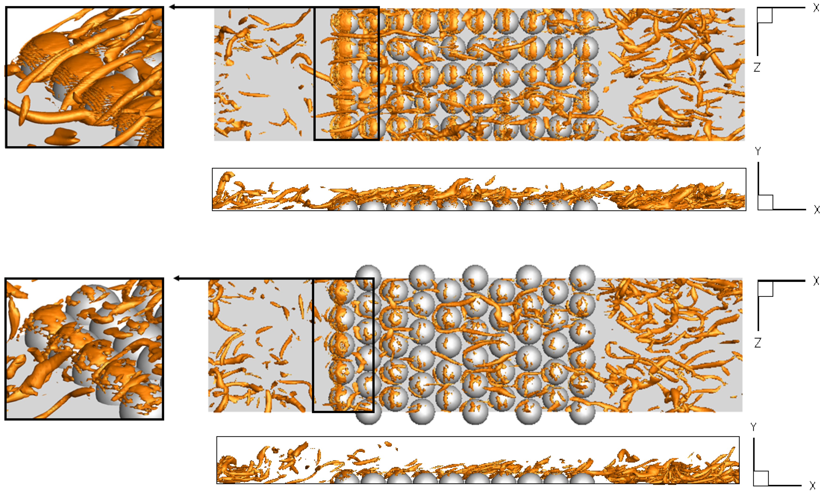
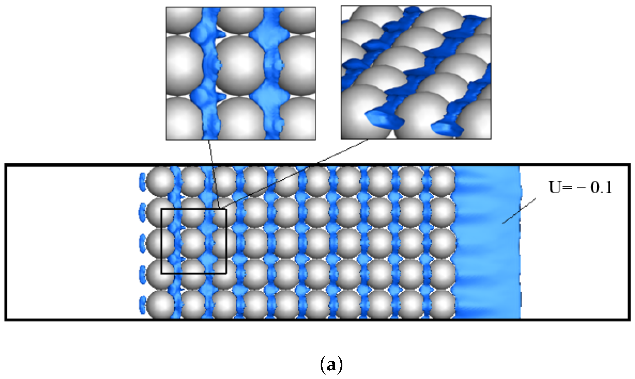
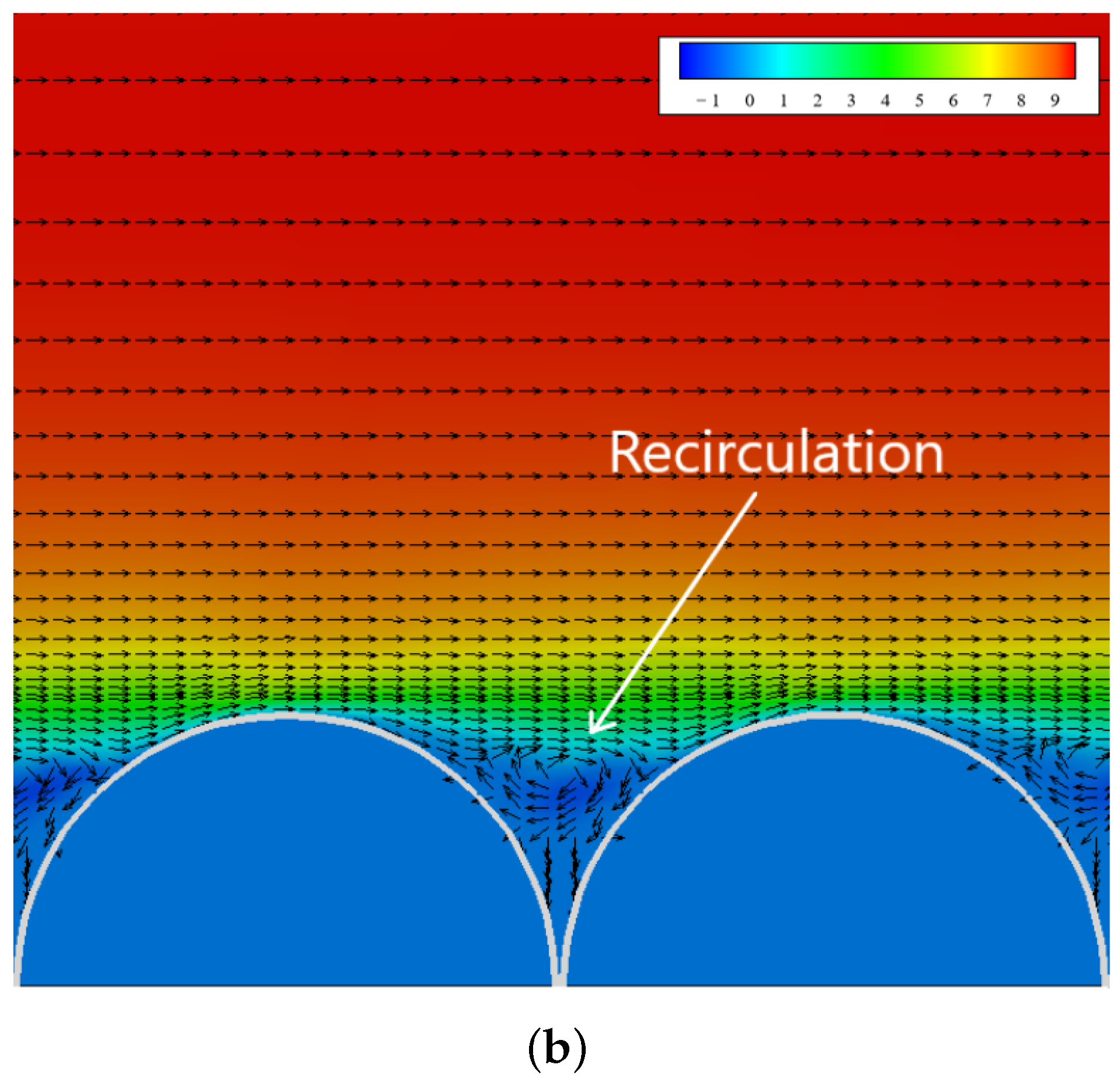
4.1. Instantaneous Flow Behavior

In all cases, the computations started with the uniform velocity in the ‘x’-direction equal to $U=15.0$, with random disturbances at the level of $0.1U$ assumed for all velocity components. These artificial fluctuations induced the appearance of natural turbulent structures and the flow adapted to the forcing imposed by the constant pressure gradient. After the initial transient phase ($t>20$), the flow could be considered as fully developed. Figure 5 shows the Q-parameter ($Q=415$) in the vicinity of the lower walls in the configurations S2.0o and S2.0s. The Q-parameter is one of the quantities that are often used to indicate vortical structures. It is defined as $Q=1/2({\mathrm{\Omega }}_{ij}{\mathrm{\Omega }}_{ij}-S_{ij}{S}_{ij})$, where $S_{ij}$ and ${\mathrm{\Omega }}_{ij}$ are the symmetrical and anti-symmetrical parts of the velocity gradient tensor. Here, the Q-parameter shows long streamwise-oriented vortices formed in between the spheres and small vortices occurring on the sphere surfaces. It can be seen that on the flat parts of the channel, flow behavior is very similar, whereas significant differences are seen in the vicinity of the spheres. In the configuration S2.0o, the number of long vortices is distinctly larger and its occurrence is more regular. In the zoomed figures of the regions of the first rows of the spheres, it can be seen that the longitudinal thin vortices originate in the gaps between the spheres. Depending on sphere arrangement, they either extend along the ‘x’-direction being pulled by the mean flow (S2.0o) or are destroyed by the subsequent row of the spheres (S2.0s). In both cases, however, these vortices reveal strongly turbulent flow behavior near the spheres.

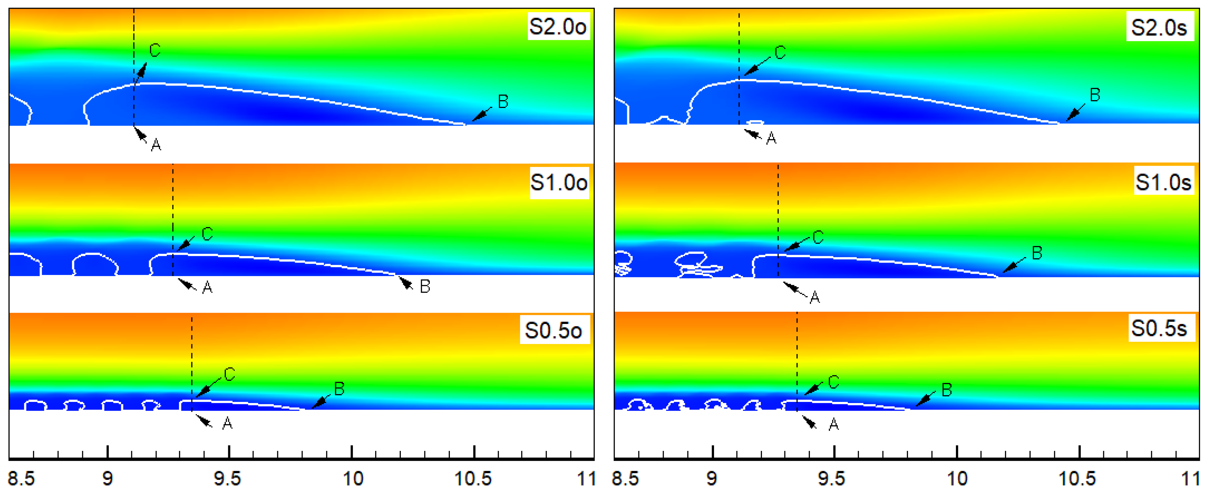
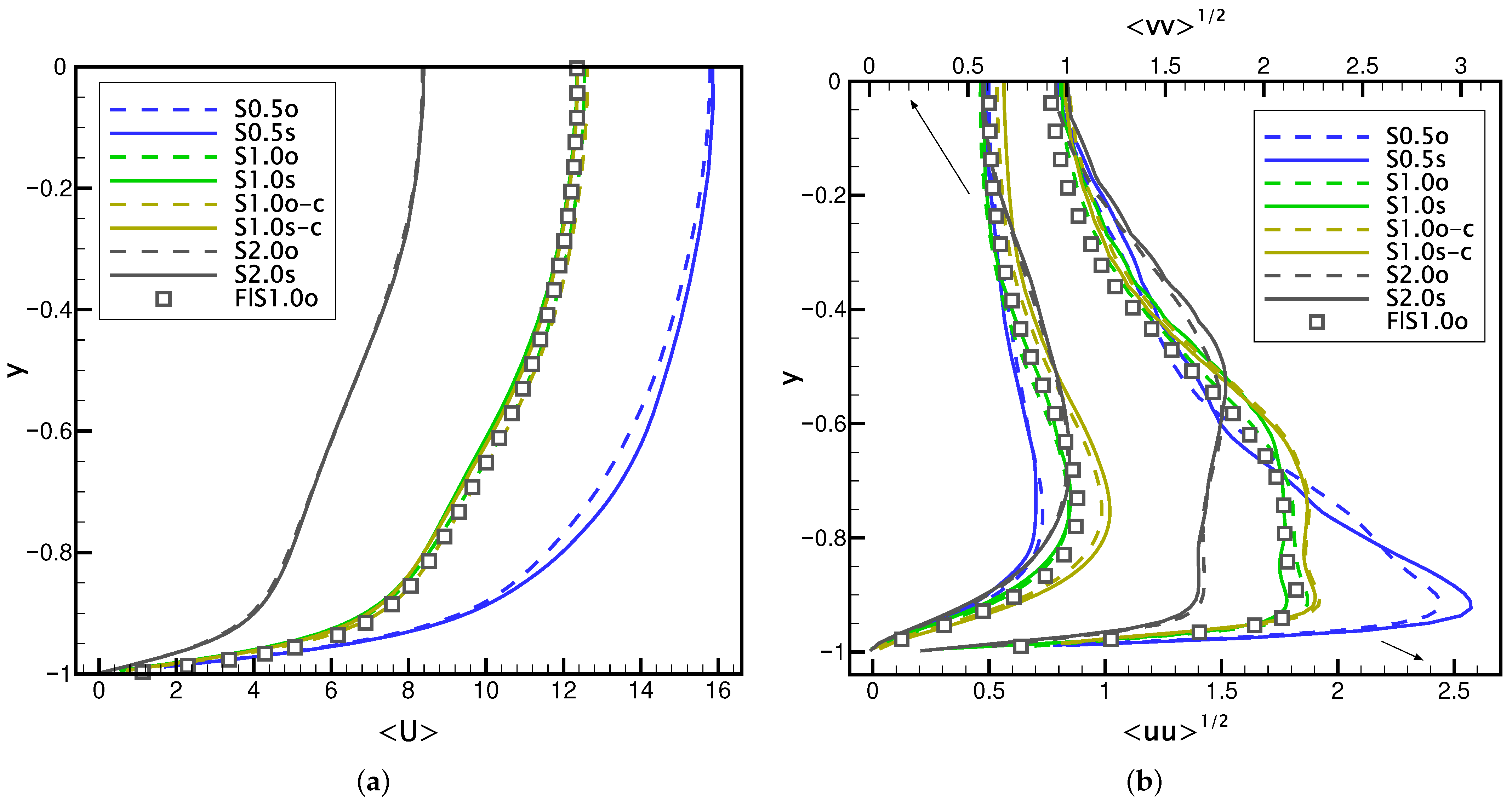
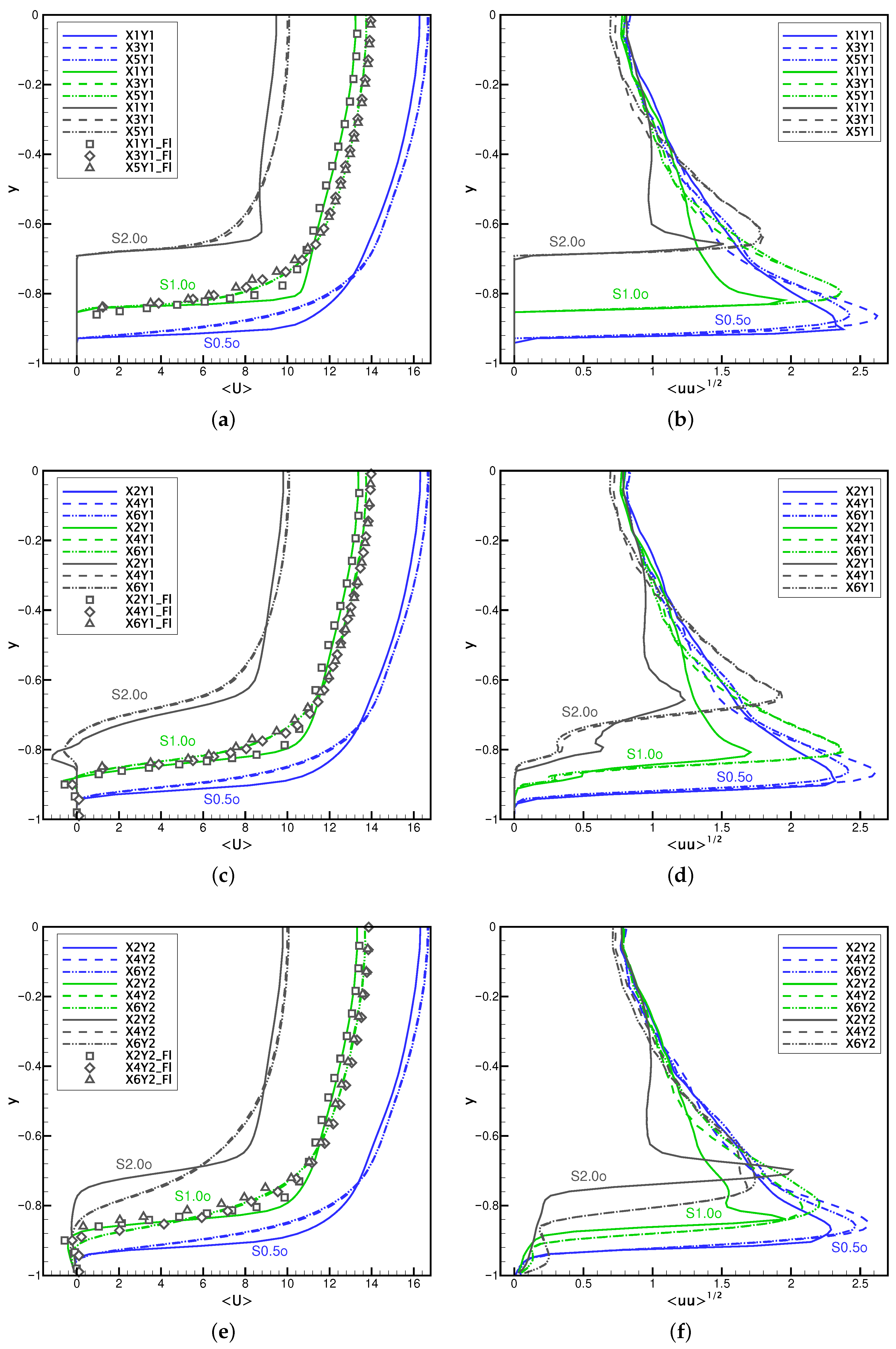
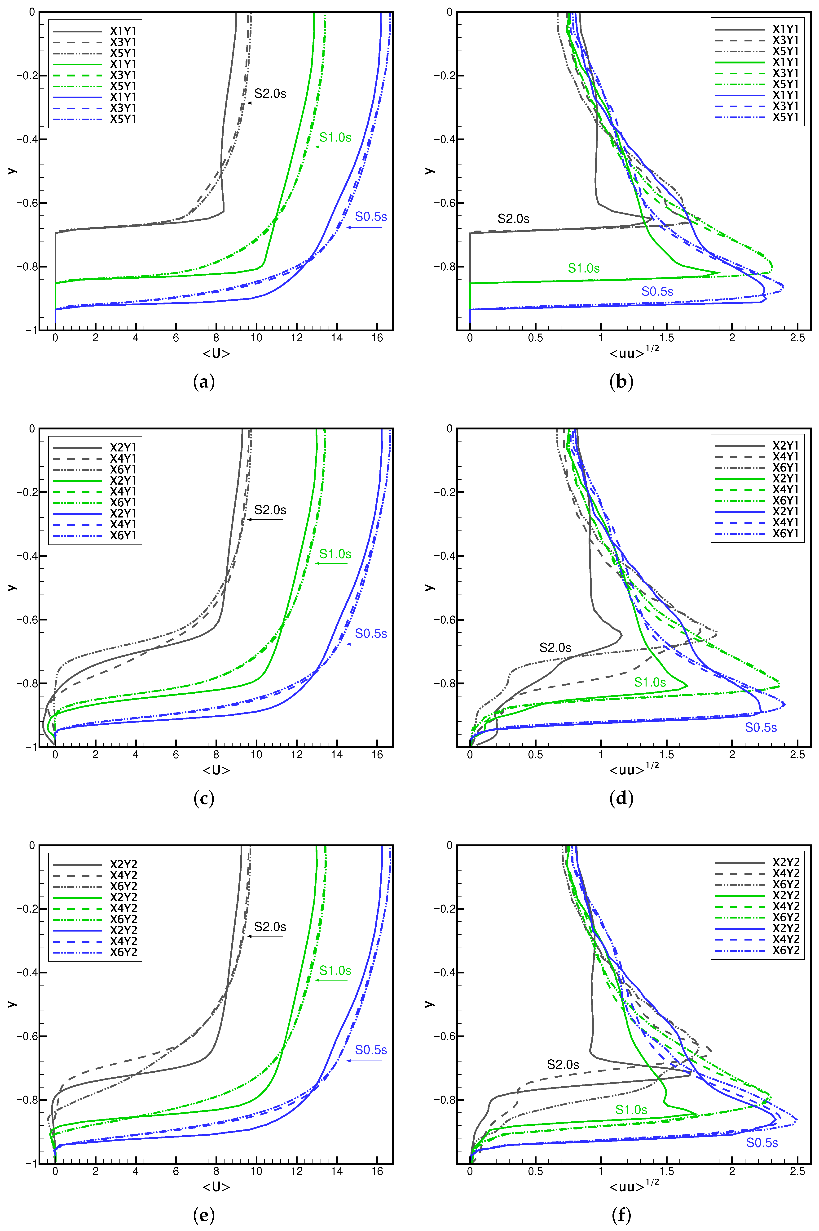
4.2. Time-Averaged Results

The time-averaging procedure was started at the time moment $t=25$ and lasted up to $t=105$, which was long enough to obtain well convergent mean quantities. Figure 6a presents the iso-surface of the time-averaged streamwise velocity equal to $\langle U\rangle =-0.1$. One can easily deduce that in the front of the first row and in between the spheres, the recirculation zones are formed that intensify the mixing process. Figure 6b presents the contours of the streamwise velocity in the ‘x-y’ cross-section plane at $z=2.5D=2.5\pi /5$ that for the case S2.0o corresponds to the localization across the spheres. The velocity vectors show how the flow recirculates in between the spheres. The sizes of the recirculation regions and the length of the recirculation zones formed downstream of the last rows of the spheres are largely dependent on the diameters of the spheres and their spatial distribution.

Figure 7 shows the contours of the time-averaged streamwise velocity that was additionally averaged along the ‘z’-direction. Point A indicates the localization of the last row of the spheres, points B and C correspond to the length and height of the recirculation zones, respectively. It can be seen that these parameters change depending on the sphere diameter and arrangement. Their detailed values are given in

Table 2. Characteristic dimensions of the recirculation zones.

Case	$\left|AC\right|$	$\left|AB\right|$	$\left|AC\right|/\left|AB\right|$	$S=1/2\left|AC\right|\left|AB\right|$
S2.0o	0.19	1.30	0.146	0.123
S1.0o	0.10	0.97	0.103	0.048
S0.5o	0.04	0.46	0.087	0.009
S2.0s	0.17	1.35	0.126	0.115
S1.0s	0.09	0.98	0.092	0.044
S0.5s	0.04	0.46	0.087	0.009

.

One can notice that in the case of the smallest spheres (S05o and S0.5s), the arrangement of the spheres (one after another or shifted) has no impact on the size of the recirculation zone. Differences are seen only when the sphere diameter is larger. In general, when the spheres are placed one after another, the recirculation zone is greater, whereas when the sphere rows are shifted, the recirculation zone is longer. In effect, the inclination angles of their upper border, approximately reflected by the ratio $\left|AC\right|$/$\left|AB\right|$, change significantly. For instance, for the cases S2.0o and S2.0s, the difference in respect to the mean value ($\left|AC\right|$/${\left|AB\right|}_{\mathrm{mean}}=0.136$) reaches $15\%$. The overall region of the recirculating flow computed as the surface area (S) of the triangles formed by the sections $\left|AC\right|$ and $\left|AB\right|$ is larger for the cases with the spheres distributed one after another. As shown by Niegodajew et al. [27], the near-wall recirculation impacts on the skin friction, with its efficient control regarded as one of the most important issues in wall-bounded flows. Hence, based on the obtained results, one can assume that the methodology of sphere distribution on the wall can be treated as one of the parameters of skin friction control.

Profiles of the Mean Velocity and Its Fluctuations

Figure 8 shows the profiles of the time-averaged streamwise velocity and the fluctuations of the streamwise and wall-normal velocity components along the channel height at $x=0,z=L_z/2$ for all analyzed configurations. The results denoted as S1.0o-c and S1.0s-c were obtained on the coarser mesh, while the square symbols denote the solutions obtained using the ANSYS Fluent code for the case S1.0o. Firstly, it can be seen that the agreement of the results is very good. Both the mean velocity and its fluctuations fit well, which confirms that the applied IB–VP method yields accurate results. Secondly, one can observe that the impact of mesh density is very small, which can be attributed to the applied high-order discretization method that, in theory, should ensure grid-independent results on moderately dense meshes. It seems that this property is well reflected in the present simulations.

Table 3. Maxima and mean values of the streamwise velocity and fluctuations of the wall-normal and streamwise velocity.

Case	$\mathrm{Max}\langle U\rangle$	$\mathrm{Mean}\langle U\rangle$	$\mathrm{Max}{\langle \mathrm{uu}\rangle }^{1/2}$	$\frac{\mathrm{Mean}{\langle uu\rangle }^{1/2}}{\mathrm{Mean}\langle U\rangle }$	$\mathrm{Max}{\langle vv\rangle }^{1/2}$	$\frac{\mathrm{Mean}{\langle vv\rangle }^{1/2}}{\mathrm{Mean}\langle U\rangle }$
S2.0o	8.435	6.259	1.509	0.156	1.014	0.094
S1.0o	12.423	10.399	1.862	0.116	1.019	0.060
S0.5o	15.869	13.394	2.429	0.099	0.877	0.047
S2.0s	8.470	6.338	1.517	0.154	1.015	0.093
S1.0s	12.623	10.239	1.887	0.120	1.019	0.063
S0.5s	15.928	13.470	2.569	0.101	0.878	0.049

shows the maxima and spatially averaged mean values of the streamwise velocity and fluctuations of the wall-normal and streamwise velocity component. Regarding the differences between the particular configurations, the following observation can be made: (i) the impact of row arrangement (one after another or shifted) is small and decreases with the increasing sphere diameter; (ii) the maxima and mean velocity values decrease with the increasing sphere diameter; this is related to different blockage of the channel, as explained in Section 3, and differences in the flow behavior between the spheres in the central part of the channel, as will be discussed later; it is worth noting that the gradient of the mean velocity profile in the vicinity of the wall increases with sphere diameter (see Figure 8a); (iii) the absolute values of the streamwise velocity fluctuations are the largest for the case S0.5; note that in the configurations S1.0 and S2.0, the fluctuation profiles are flattened in the region of $-0.9<y<-0.6$ (see Figure 8b); the wall-normal fluctuations have maximum values for the cases S1.0 and they exceed approximately 15% of the fluctuation level observed for S0.5; this means that the larger spheres induce a stronger flow in the ‘y’-direction; note that when the mean velocity fluctuations are normalized by the mean streamwise velocity, their largest values are found for the case S2.0.

Figure 9 and Figure 10 show the profiles of the time-averaged streamwise velocity and its fluctuations in the control points X1-X6 and Y1-Y2 marked in Figure 3. Note that the points X1Y1, X3Y1, and X5Y1 are placed on the centers of the sphere surface and the remaining points lie in between the spheres. The presented results were obtained for the denser mesh. For reference, the solutions obtained for the configuration S1.0o using the ANSYS Fluent code are also shown in Figure 9. Again, it can be seen that the agreement of the results is very good, and subtle differences between the profiles in different control points are accurately captured. A general remark is that in the central part of the channel, i.e., $-0.5<y<0$ the mean velocity profiles and the profiles of velocity fluctuations are not significantly dependent on sphere configuration. Although there are some evident quantitative differences between particular profiles, all solutions show similar qualitative behavior. Important differences are seen only when moving closer to the sphere surfaces. There, in addition to different values of the velocity, the character of the flow changes. In some cases, the recirculation zones appear, which is manifested as negative values of mean velocity. The fluctuation maxima significantly differ in the values and the place where they occur above the spheres. The irregularity of the fluctuation profiles increases with the sphere diameter, which can be regarded as a control parameter for turbulence intensity modulation.

The analysis of the solutions obtained for points X1Y1, X3Y1, and X5Y1 (centers of the spheres) shows that in these locations, the profiles quickly become very similar along the channel, i.e., the solutions in the points X3Y1 and X5Y1 are almost identical both for the ordered- and shifted-row configuration. The situation changes in the locations in between the spheres in the points X2, X4, and X6. In the cases S1.0o and S2.0o, mean velocity profiles reveal the occurrence of local recirculation in between $-0.86<y<-0.78$. In points X4Y1 and X6Y1, the profiles are still very similar (see Figure 9c) but the recirculation in these locations is weaker than in X2Y1, although it extends more to the central part of the channel. Note that the appearance of the recirculation in the flow around the spheres increases the shape drag. This is the second factor which, along with the larger blockage of the channel cross-section for the cases S1.0 and S2.0 causes slowing of the mean flow. The velocity fluctuations in the region of recirculation are characterized by pronounced irregularity of the profiles (see Figure 9d). Note that in the case S0.5o, there are no negative mean velocity values.

When the subsequent rows of the spheres are shifted, the mean velocity profile changes. In the configurations S1.0s and S2.0s (see Figure 10c), the recirculation in between the spheres occurs very close to the wall, which is accompanied by wavy profiles of fluctuation. The reason for that is the location of the point Y1, which, when the rows are shifted, lies in the gap behind the spheres, as can be seen in Figure 3b. This enables the development of a larger sized recirculation zone. It is worth noticing that for the case S2.0s the profiles at X2Y1, X4Y1, and X6Y1 are significantly different, particularly taking into account velocity fluctuations. This is not the case for S1.0s and S0.5s, as in these two configurations, the profiles of both mean velocity and its fluctuations at X4Y1 and X6Y1 are hardly distinguishable.

Similar conclusions can be drawn regarding the solutions in the points X2Y2, X4Y2, and X6Y2. Here, again only for the case S2.0s, the profiles at points X4Y2 and X6Y2 visibly diverge (see Figure 10e). In comparison to the solutions at points X4Y1 and X6Y1, the important differences are: (i) the near-wall recirculation zone is weaker; (ii) in the close vicinity of the spheres ($-0.8<y<-0.7$ in the case S2.0s) the mean velocity at the location X4 is the largest and it is the smallest at X6; in the cases X4Y1 and X6Y1, the opposite situation is observed, i.e., the mean velocity at the location X6 is the largest. Note, that the same behavior is found for the fluctuation profiles.

5. Conclusions

The paper presented the results of numerical simulations of the flow in a periodic channel in which the walls were covered in the central part by spherical elements that had the same overall surface areas but different radii. The computations were performed using the high-order code, whereas solid elements were modelled with the help of the immersed boundary method. For selected cases, the results were validated by comparison with the solutions obtained using the ANSYS Fluent code on the very dense body-fitted mesh. It was found that the increase of the sphere diameter causes larger overall drag force, which is attributed to the larger blockage of the channel cross-section and the occurrence of the recirculation between the large diameter spheres. In effect, with the assumed constant pressure gradient forcing term the mass flow decreases and the flow slows down. Regarding the differences between particular solutions, the velocity profiles in the vicinity of the spheres are largely dependent on sphere diameter and they rise when it increases. It was found that the distribution of the spheres plays an important role only when the spheres are large and when the recirculation zones formed behind them are characterized by different intensities and sizes. In the neighbourhood of the last rows of the spheres, the triangular recirculation zones are formed, with their height and length increasing with the sphere diameter. In the part of the channel far from the spheres, the velocity profiles seem to be independent of spheres distribution and the solutions for the cases with the ordered and shifted rows of the spheres are almost identical, yet significantly influenced by the sphere diameter. One can conclude that the placement of the spheres on the walls affects the results only in the region close to the spheres and mainly when they are large. In such cases, the distribution of the spheres could be treated as a control parameter influencing the local skin friction, and thus the drag force occurring on the sphere surfaces, and the turbulence intensity. Its efficient modulation and higher value would facilitate the control of the mixing process and heat exchange in non-isothermal flows. This subject is left for future studies.

References

1. Dróżdż, A.; Niegodajew, P.; Romańczyk, M.; Sokolenko, V.; Elsner, E. Effective use of the streamwise waviness in the control of turbulent separation. Exp. Therm. Fluid Sci. 2021, 121, 110291. [Google Scholar]
2. Chan, L.; MacDonald, M.; Ooi, A. A systematic investigation of roughness height and wavelength in turbulent pipe flow in the transitionally rough regime. J. Fluid Mech. 2015, 771, 743–777. [Google Scholar] [CrossRef] [Green Version]
3. Dharaiya, V.V.; Kandikar, S.G. A numerical study on the effects of 2d structured sinusoidal elements on fluid flow and heat transfer at microscale. Int. J. Heat Mass Transf. 2013, 57, 190–201. [Google Scholar] [CrossRef]
4. Cherukat, P.; Na, Y.; Hanratty, T.J.; McLaughlin, J.B. Direct Numerical Simulation of a Fully Developed Turbulent Flow over a Wavy Wall. Theor. Comput. Fluid Dyn. 2018, 11, 109–134. [Google Scholar] [CrossRef]
5. Kaisar, M.; Hossain, M.; Hossain, A.; Karim, A. Flow Characteristics in Convective Lid-Driven Trapezoidal Cavity with Wavy Bottom Surface. IOSR J. Mech. Civ. Eng. 2019, 16, 37–41. [Google Scholar]
6. Bhaganagar, K.; Kim, J.; Coleman, G. Effect of Roughness on Wall-Bounded Turbulence. Flow Turbul. Combust. 2004, 72, 463–492. [Google Scholar] [CrossRef]
7. Harikrishnan, S.; Tiwari, S. Heat transfer characteristics of sinusoidal wavy channel with secondary corrugations. Int. J. Therm. Sci. 2019, 145, 105973. [Google Scholar] [CrossRef]
8. Hu, Y.D.; Werner, C.; Li, D.Q. Influence of three-dimensional roughness on pressure-driven flow through microchannels. J. Fluids Eng. ASME Digit. Collect. 2003, 125, 871–879. [Google Scholar] [CrossRef]
9. Croce, G.; D’Agaro, P. Numerical analysis of roughness effect on microtube heat transfer. Superlattices Microstruct. 2004, 35, 601–616. [Google Scholar] [CrossRef]
10. Guo, L.; Xu, H.; Gong, L. Influence of wall roughness models on fluid flow and heat transfer in microchannels. Appl. Therm. Eng. 2015, 84, 399–408. [Google Scholar] [CrossRef]
11. Rawool, A.S.; Mitra, S.K.; Kandlikar, S.G. Numerical simulation of flow through microchannels with designed roughness. Microfluid. Nanofluids 2006, 2, 215–221. [Google Scholar] [CrossRef]
12. Herwig, H.; Gloss, D.; Wenterodt, T. Flow in Channels With Rough Walls–Old and New Concepts Heat Transfer Engineering. Heat Transf. Eng. 2010, 31, 658–665. [Google Scholar] [CrossRef]
13. Noorian, H.; Toghraie, D.; Azimian, A.R. The effects of surface roughness geometry of flow undergoing Poiseuille flow by molecular dynamics simulation. Heat Mass Transf. 2014, 50, 95–104. [Google Scholar] [CrossRef]
14. Croce, G.; D’Agaro, P.; Nonino, C. Three-dimensional roughness effect on microchannel heat transfer and pressure drop. Int. J. Heat Mass Transf. 2007, 50, 5249–5259. [Google Scholar] [CrossRef]
15. Zhang, Y.Z.; Sun, C.; Bao, Y.; Zhou, Q. How surface roughness reduces heat transport for small roughness heights in turbulent Rayleigh-Benard convection. J. Fluid Mech. 2018, 836, 045114. [Google Scholar] [CrossRef]
16. Anderson, W. An immersed boundary method wall model for high-Reynolds-number channel flow over complex topography. Int. J. Numer. Methods Fluids 2012, 71, 1588–1608. [Google Scholar] [CrossRef]
17. Banyassady, R.; Piomelli, U. Turbulent plane wall jets over smooth and rough surfaces. J. Turbul. 2014, 15, 186–207. [Google Scholar] [CrossRef]
18. Fletcher, C.A.J. Computational Techniques for Fluid Dynamics; Springer: Berlin/Heidelberg, Germany, 1991. [Google Scholar]
19. Tyliszczak, A. A high-order compact difference algorithm for half-staggered grids for laminar and turbulent incompressible flows. J. Comput. Phys. 2014, 276, 438–467. [Google Scholar] [CrossRef]
20. Tyliszczak, A. High-order compact difference algorithm on half-staggered meshes for low Mach number flows. Comput. Fluids 2016, 127, 131–145. [Google Scholar] [CrossRef]
21. Tyliszczak, A.; Szymanek, E. Modeling of heat and fluid flow in granular layers using high-order compact schemes and volume penalization method. Numer. Heat Transf. Part A Appl. 2019, 76, 737–759. [Google Scholar] [CrossRef]
22. Fadlun, E.A.; Verzicco, R.; Orlandi, P.; Mohd-Yusof, J. Combined immersed-boundary finite-difference methods for three-dimensional complex flow simulations. J. Comput. Phys. 2000, 161, 35–60. [Google Scholar] [CrossRef]
23. Khadra, K.; Angot, P.; Parneix, S.; Caltagirone, J.P. Fictitious domain approach for numerical modelling of Navier-Stokes equations. Int. J. Numer. Methoda Fluids 2000, 34, 651–684. [Google Scholar] [CrossRef]
24. Kadoch, B.; Kolomenskiy, D.; Angot, P.; Schneider, K. A volume penalization method for incompressible flows and scalar advection diffusion with moving obstacles. J. Comput. Phys. 2012, 231, 4365–4383. [Google Scholar] [CrossRef]
25. Tyliszczak, A.; Ksiezyk, M. Large eddy simulations of wall-bounded flows using a simplified immersed boundary method and high-order compact schemes. Int. J. Numer. Methods Fluids 2018, 87, 358–381. [Google Scholar] [CrossRef]
26. Wang, Z.J.; Fidkowski, K.; Abgrall, R.; Bassi, F.; Caraeni, D.; Cary, A.; Deconinck Hartmann, H.; Hillewaert, R.; Huynh, K.; Kroll, H.T.; et al. High-order CFD methods: Current status and perspective. Int. J. Numer. Methods Fluids 2013, 72, 811–845. [Google Scholar] [CrossRef]
27. Niegodajew, P.; Dróżdż, A.; Elsner, W. A new approach for estimation of the skin friction in turbulent boundary layer under the adverse pressure gradient conditions. Int. J. Heat Fluid Flow 2019, 79, 108456. [Google Scholar] [CrossRef]
Figure 1. Half-staggered computational mesh with a region with the red nodes belonging to the solid body. The figure on the right shows how the solid curved wall is seen on the mesh.
Processes 09 00277 g001
Figure 2. Schematic view of the computational domain with spherical elements embedded in the upper and lower walls.
Processes 09 00277 g002
Figure 3. Ordered (a) and shifted (b) arrangement of sphere rows. Subfigures show the localizations of the control points.
Processes 09 00277 g003
Figure 4. Computational meshes in the vicinity of the spheres for the configurations S0.5 (a), S1.0 with the mesh used for the computations using the ANSYS Fluent code (b) and S2.0 (c).
Processes 09 00277 g004
Figure 5. Q-parameter iso-surface in the configurations S2.0o (upper figures) and S2.0s (lower figures).
Processes 09 00277 g005
Figure 6. Iso-surface U = 0.1 of the time-averaged streamwise velocity (a) and their contours in the ‘x-y’ cross-section (b) in the configuration S2.0o
Processes 09 00277 g006aProcesses 09 00277 g006b
Figure 7. Contours of the time-averaged streamwise velocity in the ‘x-y’ plane.
Processes 09 00277 g007
Figure 8. Profiles of the time-averaged streamwise velocity (a) and the profiles of the fluctuations of the streamwise and wall-normal velocity components (b) along the channel height at x = 0 .
Processes 09 00277 g008
Figure 9. Profiles of the time-averaged streamwise velocity (a,c,e) and its fluctuations (b,d,f) along the channel height at the selected control points X and Y defined in Figure 3a. The results for the configurations S0.5o, S1.0o, and S2.0o.
Processes 09 00277 g009
Figure 10. Profiles of the time-averaged streamwise velocity (a,c,e) and its fluctuations (b,d,f) along the channel height at the selected control points X and Y defined in Figure 3b. The results for the configurations S0.5s, S1.0s, and S2.0s.
Processes 09 00277 g010