Energy Saving for Tissue Paper Mills by Energy-Efficiency Scheduling under Time-of-Use Electricity Tariffs

Abstract

Environmental concerns and soaring energy prices have brought huge pressure of energy saving and emission reduction to tissue paper mills. Electricity is one of the main energy sources of tissue paper mills. The production characteristics of tissue paper mills make it easy to decrease energy cost by using time-of-use (TOU) electricity tariffs. This study investigates the bi-objective energy-efficiency scheduling of tissue paper mills under time-of-use electricity tariffs, the objectives of which are makespan and energy cost. First, considering the processing energy cost, setup energy cost, and transportation energy cost, an energy cost model of a tissue paper mill under TOU electricity tariffs is established. Second, the energy-efficiency scheduling model under TOU electricity tariffs is built based on the energy cost model. Finally, on the basis of decomposition and teaching–learning optimization, this study proposes a novel multi-objective evolutionary algorithm and further combined with the variable neighborhood search to solve the problem. The case study results demonstrate that our study of tissue paper mill energy saving is feasible, and the proposed method has better performance than the existing methods.

1. Introduction

The paper industry is an energy-intensive industry. In 2019, its energy consumption reached 1483.2 trillion British thermal units (Btu), of which electricity consumption was 205.3 trillion Btu. [1]. At the same time, the carbon dioxide emissions of the paper industry reached 48 million tons in 2019, accounting for 4.45% of the total carbon dioxide emissions of the manufacturing industry [2]. Under the pressure from environmental degradation and rising energy costs, the papermaking industry is faced with huge energy-saving and emission reducing pressure. Studying the energy-efficiency scheduling under the time-of-use (TOU) electricity tariffs is of great significance for papermaking enterprises to improve energy efficiency. In general, one day can be divided into three periods based on the electricity demand, namely, the on-peak period, the mid-peak period, and the non-peak period. Due to the imbalance in the demand for electricity, waste will be generated in the off-peak or mid-peak periods, while the demand will exceed the supply during the on-peak period. To deal with this issue, the TOU pricing scheme is used to encourage users to use electricity in the mid-peak period and off-peak period, thus balancing the demand of electricity. In the production process, the electricity consumption of each job is different, indicating that the operation with high electricity consumption is arranged in off-peak or mid-peak periods and the operation with low electricity consumption is arranged in an on-peak period, so that the electricity cost can be decreased. The energy-efficiency scheduling under TOU electricity tariffs is based on above idea, which has attracted more attention in recent years.

Mouzon and Yildirim are the pioneers that regard energy consumption as the objective of production scheduling [3]. Energy-efficiency scheduling mainly improves energy efficiency in two ways: reducing energy consumption and reducing energy cost by scheduling. The existing research on energy-efficiency scheduling focuses on how to decrease energy consumption in different stages, such as decreasing the energy consumption in the processing stage, the setup stage, and the standby stage [4,5,6,7,8,9]. Recently, energy-efficiency scheduling decreases energy cost considering both energy consumption and energy price. Energy-efficiency scheduling under TOU electricity tariffs is an efficient way to reduce energy cost. Scholars have carried out a lot of research on energy-efficiency scheduling under TOU electricity tariffs in different generic manufacturing systems. Simple manufacturing systems, such as single machine and parallel machine, have been studied by many researchers [10,11,12,13]. However, there are few reports on complex manufacturing systems, such as flow shop, flexible flow shop, job shop, flexible job shop, etc. [14,15,16]. The generic manufacturing systems are different from the real manufacturing systems. In order to study the energy-efficiency scheduling models in line with the actual manufacturing system, some scholars have investigated energy-efficiency scheduling in the actual production and manufacturing system, such as hardware manufacturing and iron and steel industry [17,18,19,20,21,22].

According to different production stages, the energy cost mainly consists of processing energy cost, setup energy cost, standby energy cost, etc. [23]. Many studies discuss processing energy cost, which accounts for the largest proportion of the total energy cost [24,25]. Setup energy cost cannot be ignored in many industries, especially in the processing industry. In addition, transport energy cost may be negligible in many industries, but it cannot be ignored in heavy industry. Setup time and transportation time may span multiple time periods, leading to different electricity prices in the same setup stage or transportation stage. Consequently, it is difficult to build an efficient energy cost model. Many research studies on energy-efficiency scheduling under TOU electricity tariffs fails to consider the setup energy cost and the transportation energy cost.

The feasibility of reducing material wastage and energy consumption in tissue paper mills has been proved through production scheduling [26]. Energy consumption in tissue paper mills can be decreased by combining process optimization and production scheduling [27]. However, the previous research fails to consider TOU electricity tariffs. This study investigates the energy-efficiency scheduling under TOU electricity tariffs for tissue paper mills. There are three main contributions in this paper: First, a new mathematical model of energy-efficiency scheduling under TOU electricity tariffs is established for tissue paper mills. Energy cost includes processing energy cost, setup energy cost and transportation energy cost. Second, a novel Multi-Objective Evolutionary Algorithm based on Decomposition and Teaching–Learning-Based Optimization (MOEA/DTL) is proposed, which further improves the performance of the MOEA/DTL by Variable Neighborhood Search (IMOEA/DTLB). Third, the effectiveness of the proposed IMOEA/DTL is verified by carrying out a case study. Lastly, the energy-saving potential of the IMOEA/DTL is evaluated based on a practical scheduling problem in a tissue paper mill.

This paper is structured as follows. In Section 2, the production process and the energy-efficiency scheduling of tissue paper mills under electricity tariffs are described. Moreover, an energy cost model under TOU electricity tariffs is built, and the energy-efficiency scheduling model under TOU electricity tariffs is built. Section 3 introduces the proposed IMOEA/DTL method. Section 4 verifies the feasibility of the study and the effectiveness of the proposed algorithm by carrying out a case study. Finally, Section 5 summarizes the study and proposes the future research direction.

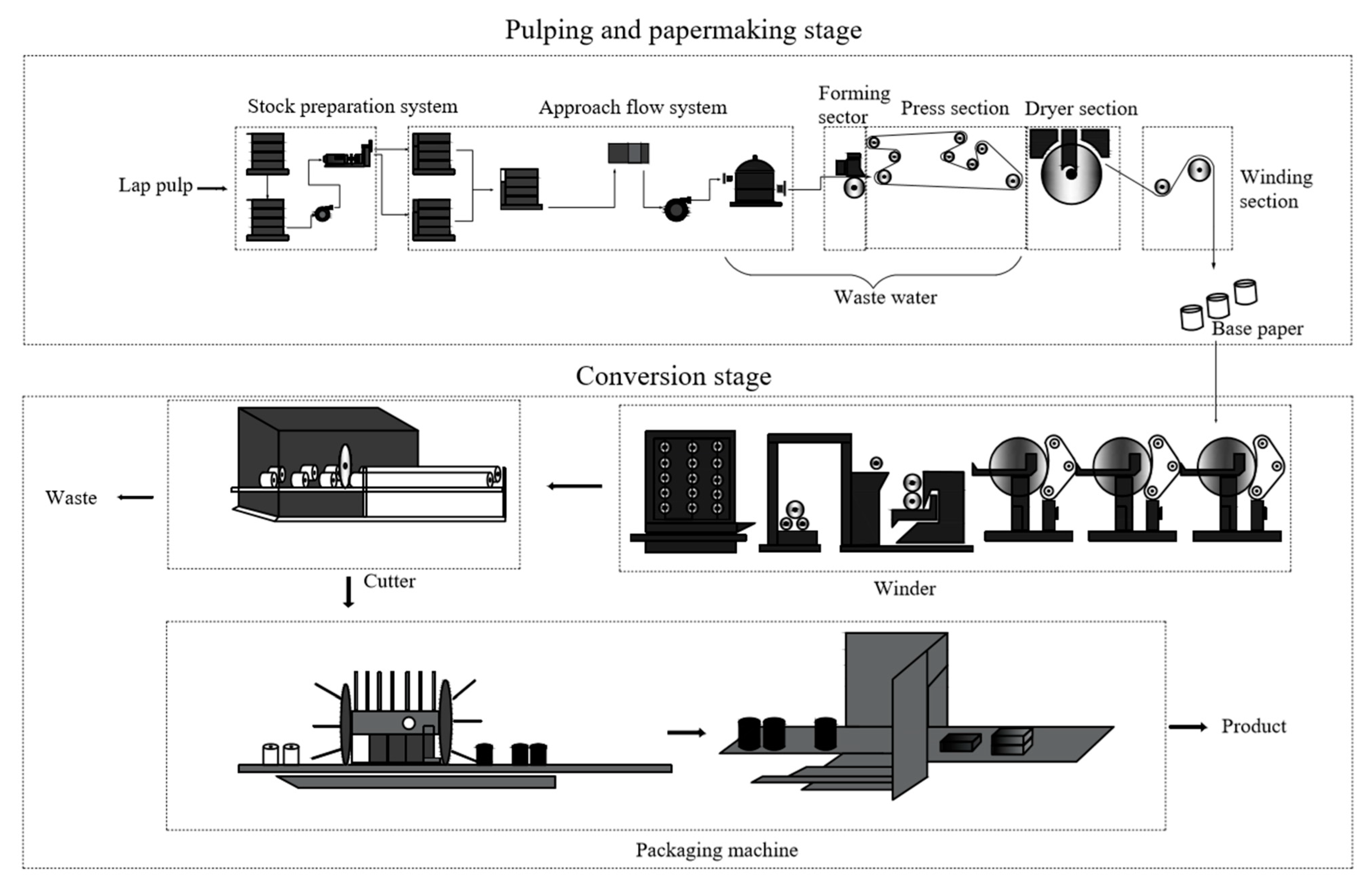
2. Problem Description and Modeling

As shown in Figure 1, the production of a tissue paper mill mainly includes two stages, namely the pulping and papermaking stage and the conversion stage. In the pulping and papermaking stage, the first production unit is the stock preparation system, which is composed of a pulper, a refiner, and a chest. The pulper is the first equipment used in the pulping and papermaking stage. The paperboard is first mixed with water and then disintegrated by the pulper to obtain the pulp with a certain concentration. The obtained pulp is stored in the chest (there are usually multiple chests). However, the quality of the pulp disintegrated by the pulper cannot meet the requirements of papermaking. Therefore, it is necessary to further improve the quality of the pulp using the refiner. The pulp obtained by the refiner will be stored in other chests. The pulper and the refiner operate intermittently, which mainly depends on the liquid level of the chest. Afterwards, the pulp is sent to the forming sector through the approach flow system. The forming sector removes part of the water, and finally, the paper is formed. Next, the paper is further dehydrated by the press section. The dryness of the paper from the press section falls far short of the requirements. Paper is dried in the dryer section to make the dryness of the paper meet the requirements. The last step of the pulping and papermaking stage is the winding section. The paper is reeled by the reel cylinder, thus forming the parent roll. The parent roll will be further processed in the conversion stage.

In the conversion stage, a certain number of parent rolls are simultaneously rolled into reels using the winder, and the number of the parent rolls depends on the numbers of paper layers in the finished product. The reel paper is cut into small reels with a cutter. Finally, the small reels are packaged into the finished product by the packaging machine. Discrete production mainly occurs in the pulping process and the processing between the pulping and papermaking stage and the conversion stage. The processing is continuous in the papermaking or conversion stage. The interval time between two stages is uncertain. Different from other flow shops, only when enough parent rolls are produced in the papermaking stage can the conversion stage be started, rather than after finishing a roll of parent roll in the papermaking stage. The interval time between two stages is related to the product characteristics and the machine speed. Too long of an interval time will increase the pressure on work-in-process inventory. However, a short interval time is likely to cause frequent downtime of the machine in the conversion stage. Therefore, it is important to determine the optimal interval time in the production scheduling.

The scheduling of a tissue paper mill, which is two-stage flexible flow shop scheduling, is composed of the pulping and papermaking stage and the conversion stage. Each job is processed by a production line in the pulping and papermaking stage and a production line in the conversion stage. The energy consumption in the processing stage accounts for the vast majority of energy consumption in tissue paper mills. Product characteristics can determine the processing energy consumption. Different product characteristics mean different process parameters, and the energy consumed by machines under different process parameters varies significantly. For example, the products with high grammage will consume more energy in the papermaking stage, and vice versa. Under TOU electricity tariffs, the energy cost can be reduced in two ways: (i) arranging the job to the production line with low processing energy consumption; and (ii) arranging the job with high grammage production in the off-peak or mid-peak period and the job with low grammage production in the on-peak period. When there are two different consecutive jobs, production changeover will occur in tissue paper mills. The parameters of the machine should be adjusted to process the new later job, which will consume a lot of energy in the setup stage. In general, the setup energy cost can be reduced by arranging jobs with lower setup energy consumption processed consecutively. Under TOU electricity tariffs, the setup energy cost can be further reduced by arranging the jobs with higher setup energy consumption processed in the off-peak or mid-peak period and the jobs with lower setup energy consumption processed in the on-peak period. The parent rolls produced in the pulping and papermaking stage should be transported to the conversion stage for further processing. The transport energy consumption is related to the distance between the papermaking line and the conversion line. Similarly, the transportation distance can be shortened to decrease the transport energy cost. Moreover, the transport energy cost can be further reduced by arranging the jobs with high transportation energy consumption in the off-peak or mid-peak period and the jobs with low transportation energy consumption in the on-peak period. Tissue paper mills can decrease the energy cost by utilizing the TOU electricity pricing scheme in job scheduling.

Table 1. Time-of-use (TOU) electricity tariffs implemented in Guangdong.

Period Type	Time Periods	Electricity Price (CNY/kWh)
Off-peak	00:00–08:00	0.3351
Mid-peak	08:00–09:00; 12:00–19:00; 22:00–24:00	0.6393
On-peak	09:00–12:00; 19:00–22:00	1.0348

shows the TOU electricity tariffs in Guangdong, China.

2.1. Energy Cost Modeling

According to the characteristics of energy consumption in tissue paper mills, this study mainly considers energy cost from three aspects: processing energy cost, setup energy cost, and transportation energy cost. Processing energy cost is related to processing energy consumption and electricity price. Under the TOU electricity pricing scheme, different electricity prices are set for different periods in a day. This study establishes a processing energy cost model combined with the TOU electricity pricing scheme and the processing energy consumption. The processing energy cost model is as below.

$$EP={\displaystyle \sum }_{j=1}^m{\displaystyle \sum }_{i=1}^n\left(EP1+EP2+EP3+EP4\right)\ast O_{i,j}$$

(1)

$$\begin{array}{c}EP1=MIN\left(CEIL\left(S_{i,j}\right)-S_{i,j},FG\left(CEIL\left(S_{i,j}+T_{i,j}\right),CEIL\left(S_{i,j}\right)\right)\right)\times U_{i,j}\\ \times P_{FLOOR\left(MOD\left(S_{i,j},K\right)\right)}\end{array}$$

(2)

$$EP2={\displaystyle \sum }_{k=CEIL\left(MOD\left(S_{i,j},K\right)\right)}^{FLOOR\left(MOD\left(S_{i,j},K\right)+\left(T_{i,j}-FIX\left(T_{i,j},K\right)\ast K\right)\right)}\left(P_k\times U_{i,j}\right)$$

(3)

$$EP3=\left(S_{i,j}+T_{i,j}-FLOOR\left(S_{i,j}+T_{i,j}\right)\right)\times U_{i,j}\times P_{FLOOR\left(MOD\left(S_{i,j}+T_{i,j},K\right)\right)}$$

(4)

$$EP4=FIX\left(T_{i,j},K\right)\times {\displaystyle \sum }_{k=1}^K\left(P_k\times U_{i,j}\right)$$

(5)

where $EP$ is the processing energy cost, and Equation (1) is the calculation formula of the processing energy cost. The processing energy cost is divided into four parts, namely $EP1$, $EP2$, $EP3$, and $EP4$. Equation (2) represents the processing energy cost from the start of the job to the next period. Equation (3) represents the processing energy cost from the next period of the start of the job to the previous period of the completion of the job. Equation (4) represents the processing energy cost from the previous period of the completion of the job to the completion of the job. If the job spans for several cycles, Equation (5) represents the processing energy cost of the job in several cycles. $m$ and $n$ are the numbers of production lines and jobs, respectively. $O_{i,j}$ denotes whether production line $j$ processes job $i$. $O_{i,j}$ is set to one when production line $j$ processes job $i$; otherwise, it is set to zero. $CEIL$ is a function that rounds up to an integer. $T_{i,j}$ is the processing time of job $i$ in production line $j$. $S_{i,j}$ is the start time of job $i$ processed in production line $j$. Function $FG$ has two parameters. When the first parameter is equal to the second parameter, $FG$ is set to one; otherwise, it is set to zero. $U_{i,j}$ represents the power of job $i$ in production line $j$, $P_k$ represents the electricity price in $k$ period. $FLOOR$ is a function that rounds down to an integer, $K$ is the number of periods, $MOD$ represents modulo operation, and $FIX$ is the quotient operation.

The setup time is up to several hours, especially in the pulping and papermaking stage, which cannot be ignored in tissue paper mills. Under the TOU electricity pricing scheme, the machine setup energy cost may be different when the setup occurs at different periods due to different energy prices in different periods. The off-peak or mid-peak period has lower setup energy cost compared with the on-peak period. Moreover, the setup may span multiple periods. The setup energy cost model is formulated as follows:

$$ES={\displaystyle \sum }_{j=1}^m{\displaystyle \sum }_{i=1}^{N_j}ES1+ES2+ES3+ES4$$

(6)

$$\begin{array}{c}ES1=MIN\left(CEIL\left(F_{i-1,j}\right)-F_{i-1,j},FG\left(CEIL\left(F_{i-1,j}+T{S}_{i,i-1,j}\right),CEIL\left(F_{i-1,j}\right)\right)\right)\\ \times U{S}_{i,i-1,j}\times P_{FLOOR\left(MOD\left(F_{i-1,j},K\right)\right)}\end{array}$$

(7)

$$ES2={\displaystyle \sum }_{k=CEIL\left(MOD\left(F_{i-1,j},K\right)\right)}^{FLOOR\left(MOD\left(F_{i-1,j},K\right)+\left(T{S}_{i,i-1,j}-FIX\left(T{S}_{i,i-1,j},K\right)\times K\right)\right)}\left(P_k\times U{S}_{i,i-1,j}\right)$$

(8)

$$\begin{array}{c}ES3=\left(F_{i-1,j}+T{S}_{i,i-1,j}-FLOOR\left(F_{i-1,j}+T{S}_{i,i-1,j}\right)\right)\times U{S}_{i,i-1,j}\\ \times P_{FLOOR\left(MOD\left(F_{i-1,j}+T{S}_{i,i-1,j},K\right)\right)}\end{array}$$

(9)

$$ES4=FIX\left(T{S}_{i,i-1,j},K\right)\times {\displaystyle \sum }_{k=1}^K\left(P_k\times U{S}_{i,i-1,j}\right)$$

(10)

where $ES$ represents the setup energy cost, and Equation (6) is the calculation formula of the setup energy cost. The setup energy cost is divided into four parts, namely $ES1$, $ES2$, $ES3$, and $ES4$. Equation (7) represents the setup energy cost from the start of the setup to the next period. Equation (8) represents the setup energy cost from the next period of the start of the setup to the previous period of the completion of the setup. Equation (9) represents the setup energy cost from the previous period of the completion of the setup to the completion of the setup. If the setup spans for several cycles, Equation (10) represents the setup energy cost of the job in several cycles. $N_j$ represents the number of jobs processed in production line $j$, $F_{i-1,j}$ is the completion time of job $i-1$ in production line $j$, $T{S}_{i,i-1,j}$ is the setup time in the conversion from job $i-1$ to job $i$ in production line $j$. $U{S}_{i,i-1,j}$ is the power when job $i-1$ is converted to job $i$ in production line $j$.

In tissue paper mills, the parent roll produced in the papermaking line should be transported to the conversion line for further processing. However, the distance between papermaking lines and conversion lines is different. The longer the distance, the higher the energy cost of transporting the parent roll from the papermaking line to the conversion line. The transportation time in tissue paper mills is up to tens of minutes. In the production scheduling process, it is necessary to consider the processing route with short distance to reduce the transportation energy cost. Under the TOU electricity pricing scheme, the transportation energy cost varies in different time periods. Similarly, the transportation time may span multiple time periods. The transportation energy cost model of tissue paper mills is formulated as below:

$$ET={\displaystyle \sum }_{i=1}^n{\displaystyle \sum }_{l=1}^{m2}\left(\left(TP1\times P1+TP2\times P2+TP3\times P3\right)\times W_i\times TC\left({\displaystyle \sum }_{h=1}^{m1}{O}_{i,h},l\right)\right)$$

(11)

$$TP1=\frac{ET1\left(1\right)+ET2\left(1\right)+ET3\left(1\right)}{{{\displaystyle \sum }}_{s=1}^3\left(ET1\left(s\right)+ET2\left(s\right)+ET3\left(s\right)\right)}$$

(12)

$$TP2=\frac{ET1\left(2\right)+ET2\left(2\right)+ET3\left(2\right)}{{{\displaystyle \sum }}_{s=1}^3\left(ET1\left(s\right)+ET2\left(s\right)+ET3\left(s\right)\right)}$$

(13)

$$TP3=\frac{ET1\left(3\right)+ET2\left(3\right)+ET3\left(3\right)}{{{\displaystyle \sum }}_{s=1}^3\left(ET1\left(s\right)+ET2\left(s\right)+ET3\left(s\right)\right)}$$

(14)

$$\begin{array}{c}ET1\left(s\right)=MIN\left(CEIL\left(S_{i,l}\right)-S_{i,l},FG\left(CEIL\left(S_{i,l}+T_{i,l}\right),CEIL\left(S_{i,l}\right)\right)\right)\\ \times Q\left(FLOOR\left(MOD\left(S_{i,j},K\right)\right),s\right)\end{array}$$

(15)

$$ET2\left(s\right)={\displaystyle \sum }_{k=CEIL\left(MOD\left(S_{i,j},K\right)\right)}^{FLOOR\left(MOD\left(S_{i,l},K\right)+\left(T_{i,l}-FIX\left(T_{i,l},K\right)\times K\right)\right)}Q\left(k,s\right)$$

(16)

$$ET3\left(s\right)=\left(S_{i,l}+T_{i,l}-FLOOR\left(S_{i,l}+T_{i,l}\right)\right)\times Q\left(FLOOR\left(MOD\left(S_{i,j},K\right)\right),s\right)$$

(17)

$$ET4\left(s\right)=FIX\left(T_{i,l},K\right)\times {\displaystyle \sum }_{k=1}^{K}Q\left(k,s\right)$$

(18)

where $ET$ is the transportation energy cost, Equations (12)–(14) calculate the proportions of the processing time of job i in the off-peak, mid-peak, and on-peak periods to the total processing time, respectively. Equation (15) represents the transportation energy cost from the start of the transportation to the next period. Equation (16) represents the transportation energy cost from the next period of the start of the transportation to the previous period of the complete of the transportation. Equation (17) represents the transportation energy cost from the previous period of the completion of the transportation to the completion of the transportation. If the transportation spans for several cycles, Equation (18) represents the transportation energy cost of the job in several cycles. $m1$ represents the number of production lines in the pulping and papermaking stage, while $m2$ is the number of production lines in the conversion stage. $TP1$, $TP2$, and $TP3$ represent the proportions of the processing time of job $i$ in the off-peak, mid-peak, and on-peak periods to the total processing time, respectively. $W_i$ is the scale of job $i$. $C\left({{\displaystyle \sum }}_{h=1}^{m1}{O}_{i,h},l\right)$ represents energy consumed by transporting job $i$ from papermaking line $h$ to conversion line $l$. The function $Q\left(k,s\right)$ can judge whether the time period $k$ belongs to period type $s$. The parameter $s$ is the period type, and $s$ values equal to 1, 2, and 3, respectively represent the off-peak, mid-peak, and on-peak period, respectively.

2.2. Energy-Efficiency Scheduling Modeling

In the pulping and papermaking stage or the conversion stage, there are multiple parallel production lines with different speeds. Each job must be first processed in a production line in the first stage and then processed in a production line in the second stage. The pulping and papermaking line or the conversion line only processes one job at a time. In this study, the job cannot be stopped once being processed in the pulping and papermaking line or the conversion line. In addition, the time interval between two stages is uncertain. The scheduling problem is the variant of a two-stage flexible flow shop scheduling problem. According to the production scheduling characteristics of tissue paper mills and the above established energy cost model, the energy-efficiency scheduling model is as below. The model in this study contains two optimization objectives, which are multi-objective optimization problems. Multi-objective optimization problems are different from single-objective optimization problems. The quality of the solution needs to be evaluated through the dominance relationship. When all the objectives of solution S1 are better than all the objectives of solution S2, it can be said that S1 dominates S2. If S1 only has some objectives better than S2, then S1 and S2 are non-dominated. If a solution is not dominated by any other solution, the solution is called a non-dominated solution. The solution to the multi-objective optimization problem is a set of non-dominated solutions.

$$\{\begin{array}{c}min\left(MAX\left(C_i\right)\right) \forall i\in \left\{1,2,\dots ,n\right\}\\ min\left(EP+ES+ET\right)\hfill \end{array}$$

(19)

$${\displaystyle \sum }_{i=1}^n{\displaystyle \sum }_{j=1}^{m1}{O}_{i,j}=1$$

(20)

$${\displaystyle \sum }_{i=1}^n{\displaystyle \sum }_{j=1}^{m2}{O}_{i,j}=1$$

(21)

$$I_{j,l}\ge F_{j,l-1}+T{S}_{l,l-1,j} \forall j\in 1,\dots ,m;\forall l\in 2,\dots ,N_j$$

(22)

$$B_{i,2}\ge B_{i,1}+f\left({\displaystyle \sum }_{l=1}^{m1}{V}_{i,l}\times O_{i,l},{\displaystyle \sum }_{h=1}^{m2}{V}_{i,h}\times O_{i,h},W_i\right) \forall i=1,\dots ,n$$

(23)

$$f\left(v1,v2,w\right)=\{\begin{array}{c}\frac{H}{v1} v1\ge v2\\ \frac{w}{v1}-\frac{w}{v2}+\frac{H}{v1} v1<v2 \end{array}$$

(24)

$$m1+m2=m$$

(25)

$${\displaystyle \sum }_{j=1}^m{N}_j=n$$

(26)

Formula (19) is the optimization objectives, and there are two optimization objectives, which are makespan and energy cost. $C_i$ is the completing time of the job i in conversion line. Constraint (20) guarantees every job can and must be processed once in the pulping and papermaking line. Constraint (21) guarantees that every job can and must be processed once in the conversion line. Constraint (22) guarantees that every papermaking line or converting line can only process one job at the same time, indicating that only when the previous job and the setup are complete can the next job be started, where $I_{j,l}$ is the beginning time of the l-th job in production line $j$. Constraint (23) guarantees there is a time interval between two stages. $B_{i,1}$ is the beginning time of job $i$ in the papermaking line, and $B_{i,2}$ is the beginning time of job $i$ in the conversion line. There is a time interval between $B_{i,1}$ and $B_{i,2}$, where $f\left({{\displaystyle \sum }}_{l=1}^{m1}{V}_l\times O_{i,l},{{\displaystyle \sum }}_{h=1}^{m2}{V}_h\times O_{i,h},W_i\right)$ represents the time interval, which is related to the speed of the papermaking line $l$ when processing job $i$ ($V_{i,l}$), the speed of the conversion line $h$ when processing job $i$ ($V_{i,h}$), and the scale of job ($W_i$). Formula (24) is the calculation method of the time interval between $B_{i,1}$ and $B_{i,2}$, where $H$ represents the value of the length of the parent roll multiplying the number of paper layers in finished products. Formulas (25) and (26) are equality constraints.

3. The Proposed Optimization Algorithm

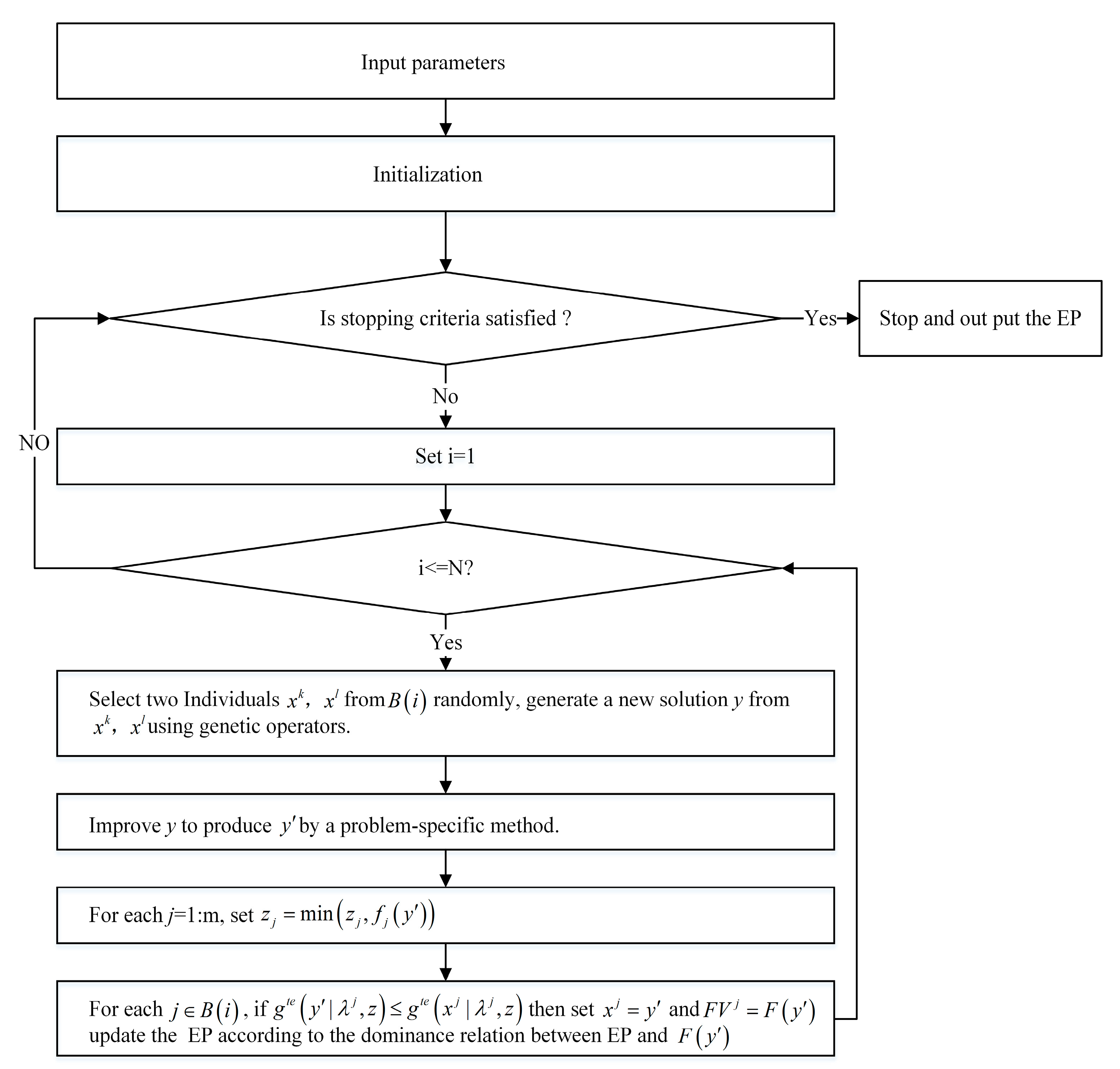
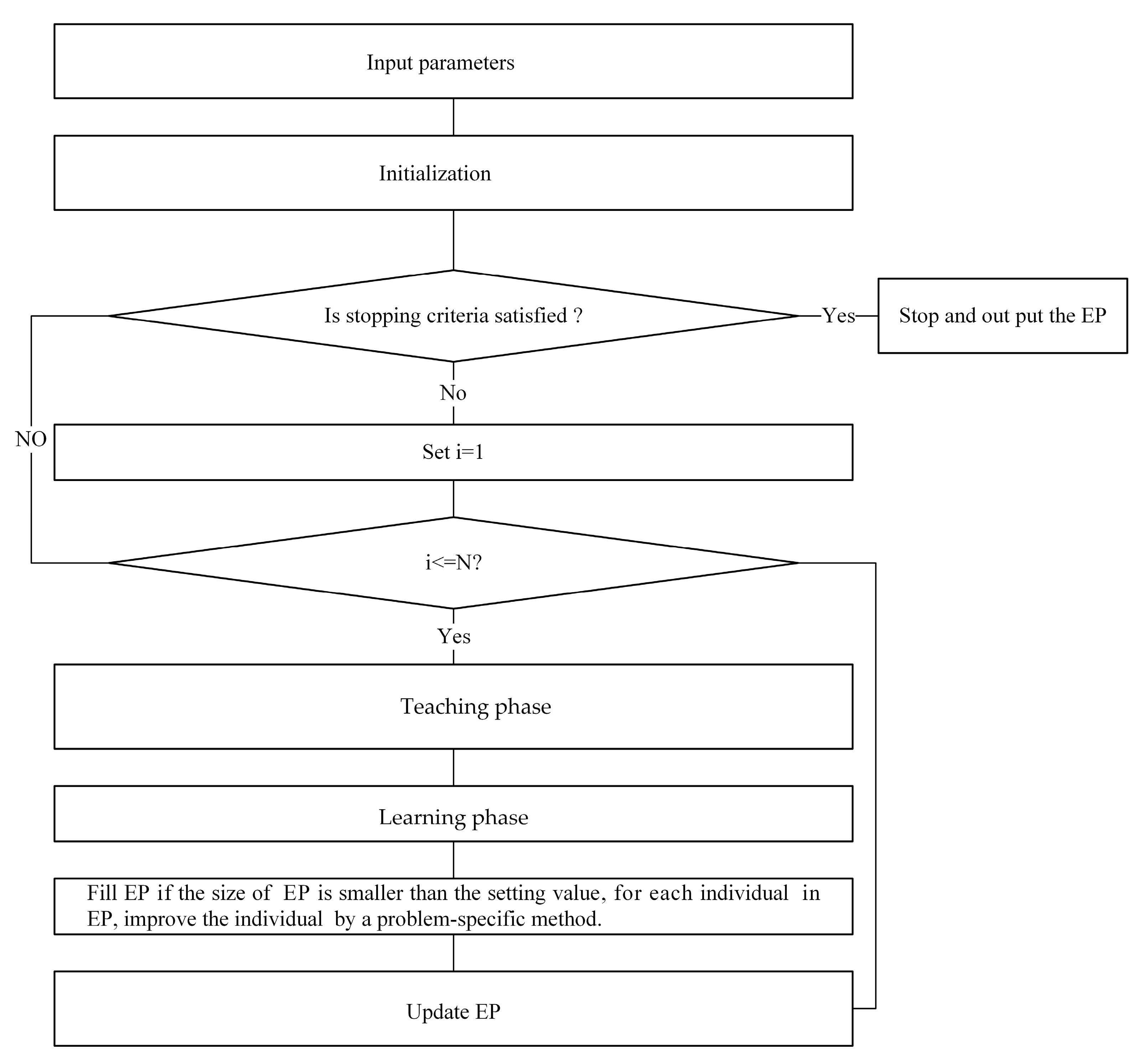
In this section, the MOEA/DTL is proposed based on two outstanding methods, namely teaching-learning-based optimization (TLBO) and MOEA/D. In order to further improve the quality of the solutions, a variable neighborhood search (VNS) algorithm is designed to be combined with the MOEA/DTL to improve the performance of the algorithm (IMOEA/DTL).

3.1. MOEA/DTL

MOEA/D uses multiple weight vectors to decompose the multi-objective optimization problem into multiple single-objective sub-optimization problems. When the weight vectors are distributed uniformly, the MOEA/D assumes Pareto optimal solutions with uniform distribution generated by combining the solutions of sub-optimization problems. Every individual is corresponding to a sub-optimization problem in MOEA/D. In each iteration of MOEA/D, each individual exchanges information with neighbors and coevolves [28]. The flow chart of the standard MOEA/D is shown in Figure 2.

The input parameters are consistent with the input parameters of the proposed algorithm; refer to the input parameters of the proposed algorithm below. The initialization is the same as the proposed algorithm; refer to the proposed algorithm below. $g^{te}\left(x^i|{\lambda }^i,z\right)$ is the decomposition approach. There are many decomposition approaches; among them, the boundary intersection approach, Tchebycheff approach, and weighted sum approach are three popular decomposition approaches.

The basic idea of TLBO is to simulate the learning process of the class, which is completed in two phases: the teaching phase and the learning phase. Each individual learns from the teacher (the best individual is selected as the teacher) in the teaching phase. Individuals learn from each other (an individual is randomly selected) in the learning phase. The TLBO is originally designed to solve the continuous optimization problem because the formulas used to update individuals in the teaching and learning phase are continuous variable oriented. Some changes should be made when the scheduling problem is solved by the TLBO. This study modifies the TLBO by replacing the update formula by the discrete crossover operation. According to the idea of MOEA/D and TLBO, this study proposes a hybrid method (MOEA/DTL). The Figure 3 shows the flow chart of MOEA/DTL. The details of the proposed MOEA/DTL are shown in Algorithm 1.

Algorithm 1 MOEA/DTL

1. Initialize the population scale and the number of subproblems.   2. Initialize the maximum number of iterations (Mt).   3. Initialize a set of $N$ weight vectors with uniform distribution (${\lambda }^1,{\lambda }^2,\dots ,{\lambda }^N$).   4. Initialize the number of neighbors for every weight vector (T).   5. Set the external population $EP=\mathsf{\Phi }$.   6. for each $i=1 to N$do   7.   The nearest $T$ weight vectors of the i-th weight vector is calculated according to Euclidean distances.   8.   Set $B\left(i\right)=\left\{{\lambda }_1^i,{\lambda }_2^i,\dots ,{\lambda }_T^i\right\}$, where $B\left(i\right)$ is the neighbors of ${\lambda }^i$ with $T$ weight vectors.   9. end for 10. Generate $x^1,x^2,\dots ,x^N$ by a specific method. 11. $F{V}^i=F\left(x^i\right)$ is set by the decomposition approach. 12. Set $z={\left(z_1,z_2,\dots ,z_n\right)}^T$, where $z_j=mi{n}_{1\le i\le N}\left(f_j\left(x^i\right)\right)$, $f_j\left(x^i\right)$ is the j-th objective of solution $x^i$. 13. while true do 14.  for $i=1 to N$ do 15.   Teaching phase: 16.   if $x^i$ is not the best individual among its $T$ neighbors 17.    An individual from its $T$ neighbors is randomly set as teacher $Th$ with a       probability Ps, or an individual is randomly selected from $EP$ as teacher $Th$ with a       probability 1-Ps. 18.   else 19.    An individual is randomly selected from $EP$ as $Th$. 20.   end if 21.   A new individual $y$ is generated by a crossover operation from $x^i$ and $Th$. 22.   Mutation operation is applied to $y$ with probability $Pm$ to generate a new individual $y^{\prime }$. 23.   for each $j\in [1,\dots ,m]$ do 24.    Set $z_j=min\left(z_j,f_j\left(y^{\prime }\right)\right)$. If $g^{te}\left(y^{\prime }|{\lambda }^i,z\right)\le g^{te}\left(x^i|{\lambda }^i,z\right)$, set $x^i=y^{\prime }$ and $F{V}^i=F\left(y^{\prime }\right)$. 25.   end for 26.   Learning phase: 27.   for each $j\in B\left(i\right)$ do 28.    if $x^j$ is not the best individual in the $T$ neighbors of $x^i$ 29.     A new individual $y^{″}$ is first generated by crossover operation from $x^i$ and $x^j$. 30.     A new individual $y^{‴}$ is generated by applying the mutation operation to $y^{″}$ with probability $Pm$. 31.    else 32.     Continue to the next iteration. 33.    end if 34.    for each $j\in \left[1,\dots ,m\right]$do 35.     set $z_j=min\left(z_j,f_j\left(y^{\prime }\right)\right)$. 36.     if $g^{te}\left(y^{‴}|{\lambda }^i,z\right)\le g^{te}\left(x^i|{\lambda }^i,z\right)$ 37.      Set $x^i=y^{‴}$ and $F{V}^i=F\left(y^{‴}\right)$. 38.     end if 39.    end for 40.   end for 41.  end for 42.  Update $EP$: a new non-dominated set is selected from $EP$ and the new population as the     new $EP$, and get rid of the duplicate solution. If the size of $EP$ is smaller than the setting     value, some randomly generated individuals ($E{P}^{\prime }$) are added to $EP$ until the size of     $EP$ is equal to the setting value. 43.  for each $i=1 to size\left(EP\right)$ do 44.   An individual $x^i$ is randomly selected from $EP-E{P}^{\prime }$, and an individual $x^j$ is ran-      bdomly selected from $EP-E{P}^{\prime }$ with a probability $Pc$, or an individual $x^j$ is selected      from $E{P}^{\prime }$ with a probability $1-Pc$. 45.   A new $y$ is generated by crossover operation from $x^i$ and $x^j$. 46.   Mutation operation is applied to $y$ with probability $Pm$ to generate a new $y^{\prime }$. 47.  end for 48.  Update $EP$: select a new non-dominated set from $EP$ and the new population as the new $EP$ 49.  if the stopping criterion is not satisfied 50.   Continue. 51.  else 52.   Stop and output $EP$. 53.   end if 54. end while

The weight vectors can determine the quality of solution obtained by MOEA/DTL. With the uniformly distributed weight vectors, the solution obtained by MOEA/DTL is more evenly distributed and closer to the Pareto optimal solution. Thus, the method of generating some weight vectors with even distribution is of great importance to MOEA/DTL. In this study, a number of weight vectors are generated as follows:

• Step (1) Set $\gamma =\left({\gamma }^1,{\gamma }^2,\dots ,{\gamma }^{N+1}\right)$, where ${\gamma }^i=\left({\gamma }_1^i,{\gamma }_2^i\right)$ For each $i=0 to N$, do:

${\gamma }_1^i=\frac{i}{N}$, ${\gamma }_2^i=1-\frac{i}{N}$.

• Step (2) Generate weight vectors $\lambda =\left({\lambda }^1,{\lambda }^2,\dots ,{\lambda }^N\right)$ by randomly selecting $N$ vectors from $\gamma$.

The parameter Ps is one of the important factors affecting the convergence speed of the algorithm. If Ps is too small, it means that most of the teachers are from the global optimal individual, and it is easy to fall into the local optimal value. If Ps is too large, it means that most of the teachers come from the best individuals in the neighborhood, and the convergence speed will be slower. The value of Ps between 0.7 and 0.9 is reasonable. The decomposition approach is also important for MOEA/DTL. The makespan and the energy cost are converted into an objective using the weighted sum approach. The makespan and the energy cost are the two different scalar objectives. Therefore, the decomposition method must have the function of normalization. The decomposition approach is as below:

$$g^i={\displaystyle \sum }_{j=1}^m\frac{{\lambda }_j^i\times \left(f_j\left(x^i\right)-f_j^{min}\right)}{f_j^{max}-f_j^{min}}$$

(27)

where $g^i$ is the scalar optimization objective of solution $x^i$, $f_j^{max}$ is the maximum of the j-th objective, and $f_j^{min}$ is the minimum of the j-th objective.

3.2. Variable Neighborhood Search

With the advantages of high efficiency and simple implementation, the Variable Neighborhood Search (VNS) algorithm has been successfully applied in many engineering fields [29,30]. The VNS algorithm uses the neighborhood structure of different actions to search alternately, thus achieving a good balance between concentration and evacuation. Firstly, the VNS is carried out in a small neighborhood. If the quality of the solution cannot be improved, VNS will be carried out in a larger neighborhood. When a better solution is found, the VNS is conducted in a smaller neighborhood again. The cycle is repeated until the end of the algorithm. The VNS algorithm is simple in principle, easy to implement, and has good optimization performance. The procedure of the VNS algorithm used in this paper is shown in Algorithm 2:

Algorithm 2 VNS

1. Construct the set of neighborhood structures $S_i$, $i=1,2,3$. 2. Set the maximum iterations $M$ for searching in the first, second, and third neighborhood structures $M1$, $M2$, $M3$. 3. Set the initial solution. 4. for each $i\in \left[1,2,\dots ,M\right]$ do 5.  for each $j\in \left[1,2,\dots ,M1\right]$ do 6.   Based on the current solution, the first neighborhood structure $S_1$ is used to search for     better solutions than the current solution, and it means that the solutions found can     dominate the current solution. 7.  end for 8.  for each $j\in \left[1,2,\dots ,M2\right]$ do 9.   Based on the current solution, the second neighborhood structure $S_2$ is used to search     for better solutions than the current solution, and it means that the solutions found can     dominate the current solution. 10.  end for 11.  for each $j\in \left[1,2,\dots ,M3\right]$ do 12.   Based on the current solution, the third neighborhood structures $S_3$ is used to search      for better solutions than the current solution, and it means that the solutions found can      dominate the current solution. 13.  end for 14.  If the stopping criteria are not satisfied, continue; otherwise, stop and output the best solution. 15. end for

The core of the VNS algorithm lies in the design of neighborhood structure set. In the production scheduling, the neighborhood structure of VNS can be obtained by exchanging the order of two jobs or inserting one job before another. This study designs three neighborhood structures, which are $S_1$, $S_2$, and $S_3$. The neighborhood solutions of $S_1$ are generated as follows: select two jobs randomly and exchange their positions to generate a new neighborhood solution. The neighborhood solutions of $S_2$ are generated as follows: select three jobs randomly and then disrupt their order to generate five new neighborhood solutions. The neighborhood solutions of $S_3$ are generated as follows: select four jobs randomly and then disrupt their order to generate 23 new neighborhood solutions. The parameters M, M1, M2, and M3 affect the search range. A large value means a large search range, but at the same time, it reduces the operating efficiency of the algorithm. On the contrary, the operating efficiency of the algorithm will improve, but it means that the search range becomes smaller. In order to balance the two, it is reasonable to set their value within 10.

3.3. IMOEA/DTL

Despite the outstanding global search capability of MOEA/DTL, it is likely to miss the locally better solution because MOEA/DTL does not search the neighborhood of the solution in detail in each iteration process. The MOEA/DTL is combined with VNS (IMOEA/DTL) to enhance its local search ability and performance. In IMOEA/DTL, the solution obtained in each iteration of MOEA/DTL is searched locally using the VNS algorithm to find a better solution. This study carries out VNS after the first update of EP, and VNS is carried out as Algorithm 3.

Algorithm 3 Combination method of VNS and MOEA/DTL

1. for each $i\in \left[1,2,\dots ,N\right]$ do 2.  $nex\_x^i=VNS\left(x^i\right)$ 3. end for 4. Output the new population.

4. Case Study

In order to demonstrate the feasibility of the energy-efficiency scheduling model under TOU electricity tariffs for tissue paper mills and the superiority of the proposed IMOEA/DTL, three popular multi-objective optimization algorithms, namely, MOEA/D-MR [31], Non-dominated Sorting Genetic Algorithm II (NSGA-II), and Strength Pareto Evolutionary Algorithm 2 (SPEA2), are compared with the IMOEA/DTL in eight scheduling problems. The energy-saving potential of the IMOEA/DTL is evaluated by comparing IMOEA/DTL with workers in practice. The whole experiments are implemented in MATLAB 2015b.

4.1. Experiment Data

The data are collected from a tissue paper mill in Guangdong, China. The data are collected from the Jiangmen branch of Vinda Paper (China) Co., Ltd., Jiangmen City, Guangdong Province, China. The data collection time is from 2017 to 2018. The scheduling data and product process data are mainly collected from the production scheduling department. These data come from the enterprise resource planning system. Machine data and energy consumption data are automatically collected by the manufacturing execution system. There are six production lines in the pulping and papermaking stage and seven production lines in the conversion stage. A total of 16 scheduling instances are generated randomly, the numbers and names of jobs in each scheduling problem are listed in

Table 2. The name and number of jobs of 16 scheduling problems.

Problems	Job Number
Job1	50
Job2	60
Job3	70
Job4	80
Job5	90
Job6	100
Job7	110
Job8	120
Job9	130
Job10	140
Job11	150
Job12	160
Job13	170
Job14	180
Job15	190
Job16	200

. In each scheduling problem, the size of each job is generated randomly and obeys uniform distribution in the range of [10,000, 600,000]. In the tissue paper mill, the speed of the production line varies with the type of products, but each production line has a maximum speed. The maximum speeds in the pulping and papermaking stage and the conversion stage are shown as

Table 3. The maximum speed of the production line in the pulping and papermaking stage and the converting stage.

Pulping and Papermaking Stage	Speed (m/min)	Converting Stage	Speed (bag/min)
PL1	990	BL1	260
PL2	950	BL2	320
PL3	1010	BL3	330
PL4	970	BL4	325
PL5	1050	BL5	335
PL6	1110	BL6	360
		BL7	400

. Similarly, the power of each production line also varies with the product type. The maximum power of the pulping and papermaking stage and the conversion stage is shown

Table 4. The maximum power of the production line in the pulping and papermaking stage and the converting stage.

Pulping and Papermaking Stage	Power (kW)	Converting Stage	Power (kW)
PL1	1210	BL1	130
PL2	1280	BL2	145
PL3	1380	BL3	148
PL4	1470	BL4	120
PL5	1330	BL5	138
PL6	1490	BL6	135
		BL7	137

. The setup energy consumption is dependent on the setup time and the setup power. In this study, the setup time of the pulping and papermaking stage and the conversion stage is randomly generated based on the real situation. The setup time of the pulping and papermaking stage shows uniform distribution in the range of [10, 100], while the setup time of the conversion stage shows uniform distribution in the range of [10, 60].

Table 5. The setup power of the production line in the pulping and papermaking stage and the converting stage.

Pulping and Papermaking Stage	Power (kW)	Converting Stage	Power (kW)
PL1	813	BL1	82
PL2	821	BL2	97
PL3	878	BL3	104
PL4	902	BL4	70
PL5	870	BL5	87
PL6	922	BL6	91
		BL7	88

lists the setup power of the pulping and papermaking stage and the conversion stage. The transportation energy consumption is related to the distance between production lines. The transportation energy consumption per unit product is shown in

Table 6. The transportation energy consumptions per unit product (kW).

	BL1	BL2	BL3	BL4	BL5	BL6	BL7
PL1	4	6	16	17	18	20	24
PL2	5	3	15	16	19	23	25
PL3	16	18	3	4	6	19	21
PL4	17	15	5	2	3	15	16
PL5	26	27	22	20	17	4	3
PL6	27	26	23	21	18	3	5

.

4.2. Performance Metrics

The performance of the IMOEA/DTL, MOEA/D-MR, NSGA-II, and SPEA2 is evaluated using two metrics, which are Hypervolume indicator (HV-metric) and Set Coverage (C-metric). C-metric reflects the dominance between two non-dominated solution sets. $A$ and $B$ represent two non-dominated solutions, $C\left(A,B\right)$ can be defined as the proportion of solutions in $B$ that are dominated by at least one solution in $A$. The formulation of $C\left(A,B\right)$ is shown as follows.

$$C\left(A,B\right)=\frac{\left|\left\{b\in B|a\in A:a\succ b\right\}\right|}{\left|B\right|}$$

(28)

The $C\left(A,B\right)$ equal to one means that all solutions in $B$ are dominated by some solutions in $A$. Meanwhile, $C\left(A,B\right)$ equal to zero means there is no solution in $B$ dominated by the solutions in $A$. When $C\left(A,B\right)$ is greater than $C\left(B,A\right)$, then the quality of the solution $A$ is better than that of $B$.

The HV-metric of a non-dominated set can be represented by the size of portion of objective space that is dominated by those solutions collectively and bounded above by a reference point. The HV-metric can not only assess the proximity of the non-dominated set but also can assess the diversity of the non-dominated set. The HV-metric needs to be given a reference point, where we use the maximum value of the solutions obtained by all algorithms. When the HV-metric has a larger value, the approximate non-dominated solution set is better.

Moreover, considering the randomness of the evolutionary algorithm, this study carries out the Wilcoxon signed-rank test to detect whether the results obtained by different algorithms are different significantly. The significance level is 0.05. A p-value of the Wilcoxon signed-rank test less than 0.05 indicates significant differences between the two algorithms.

4.3. Parameters Setting

Table 7. Parameters setting of MOEA/D-MR, Strength Pareto Evolutionary Algorithm 2 (SPEA2), Non-dominated Sorting Genetic Algorithm II (NSGA-II), and MOEA/DTL by Variable Neighborhood Search (IMOEA/DTL).

MOEA/D-MR	SPEA2	NSGA-II	IMOEA/DTL
N: 100 Mt: 100 F: 0.5 CR: 0.2 H: 99 Tm: 10 Tr: 10	N: 100 Size of archive: 100 Mt: 100 Pc: 0.8 Pm: 0.2	N: 100 Mt: 100 Pc: 0.8 Pm: 0.2	N: 100 Mt: 100 Size of EP: 100 T: 10 Ps: 0.7 Pm: 0.3 Pc: 0.7 M: 5 M1: 10 M2: 5 M3: 3

summarizes the parameters of IMOEA/DTL, MOEA/D-MR, SPEA2, and NSGA-II. The population size and the maximum iterations are set as the same value to compare the performance of IMOEA/DTL, MOEA/D-MR, SPEA2, and NSGA-II. The parameters of NSGA-II, SPEA2, and MOEA/D-MR are set based on some literature and the trial and error method [31,32,33,34,35]. Moreover, considering the randomness of the evolutionary algorithm, three algorithms are run ten times for each scheduling problem, and the result is the average of ten times.

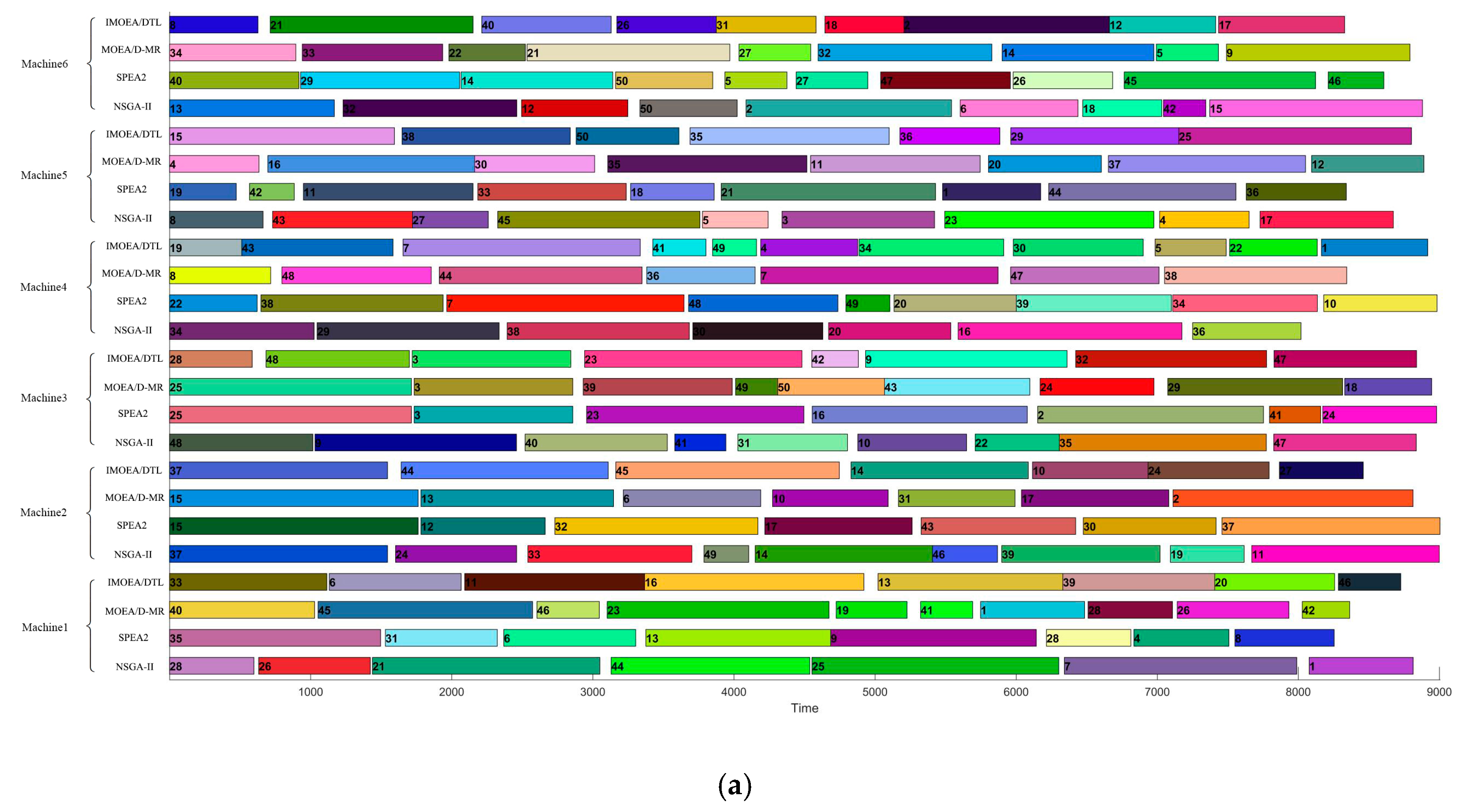
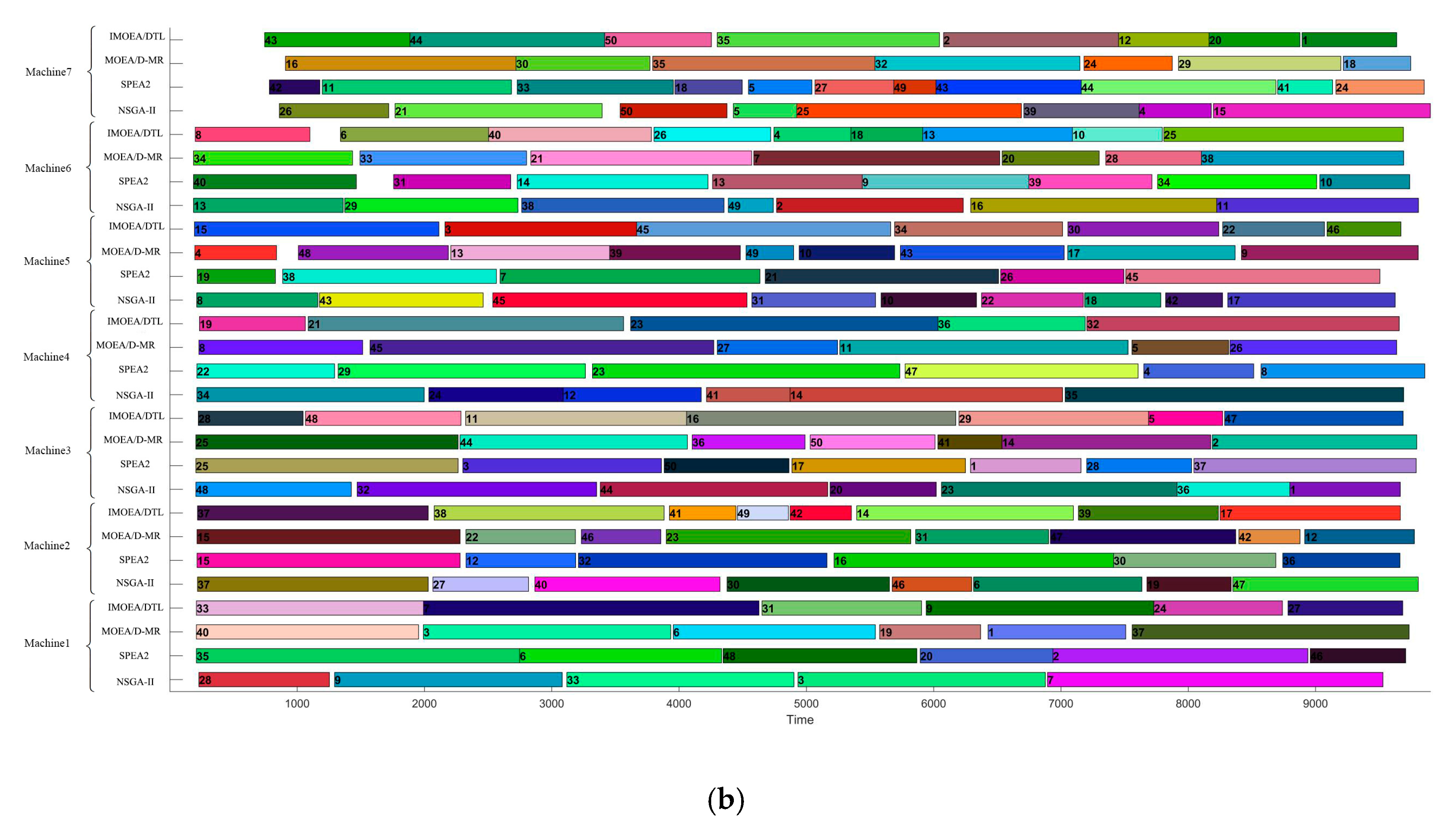
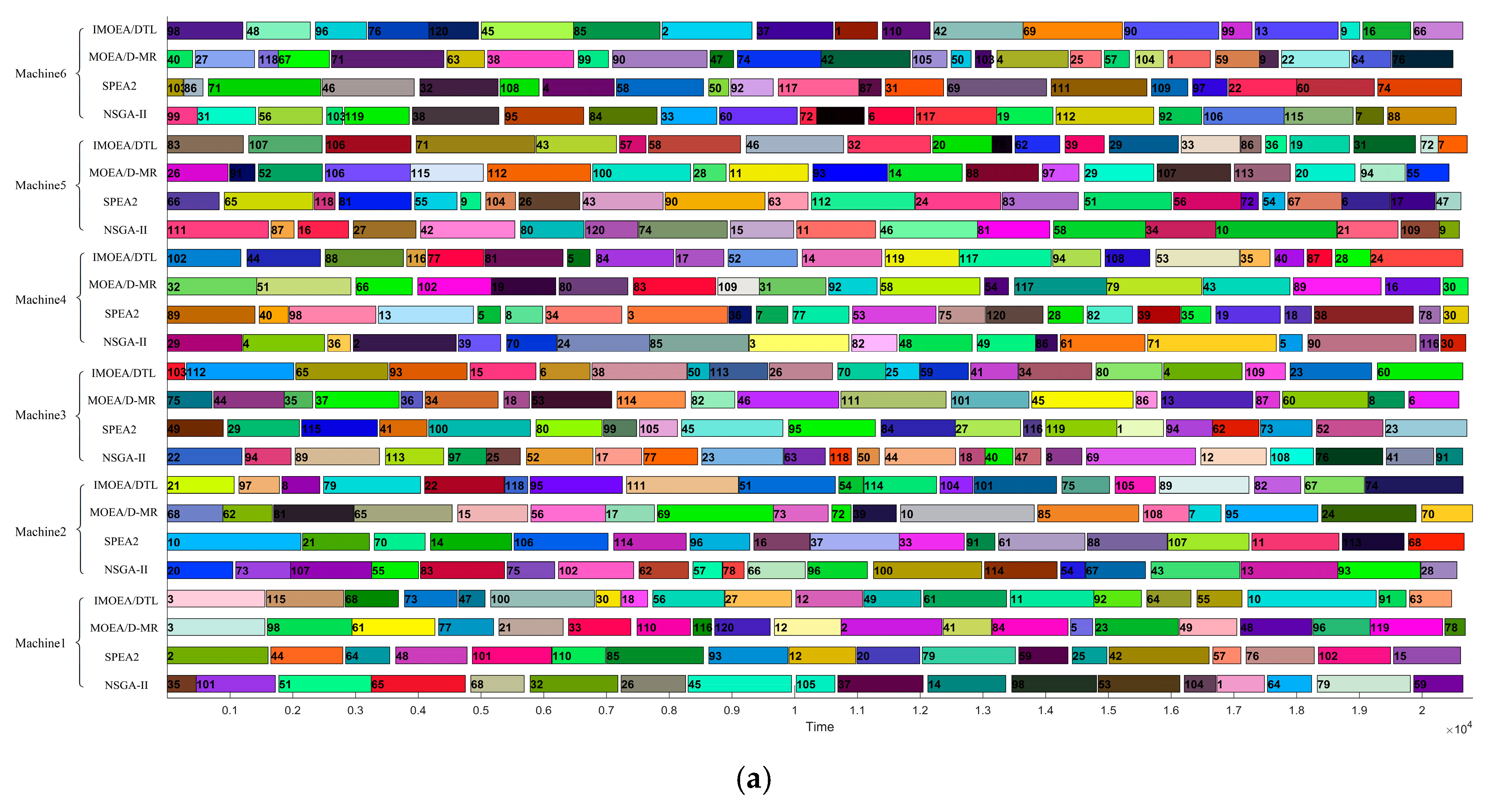
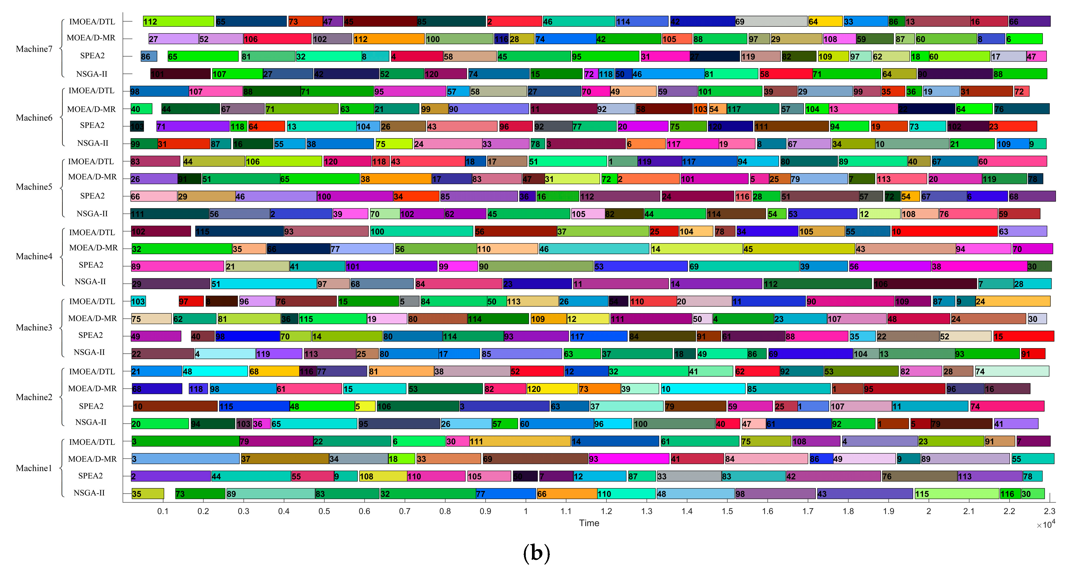
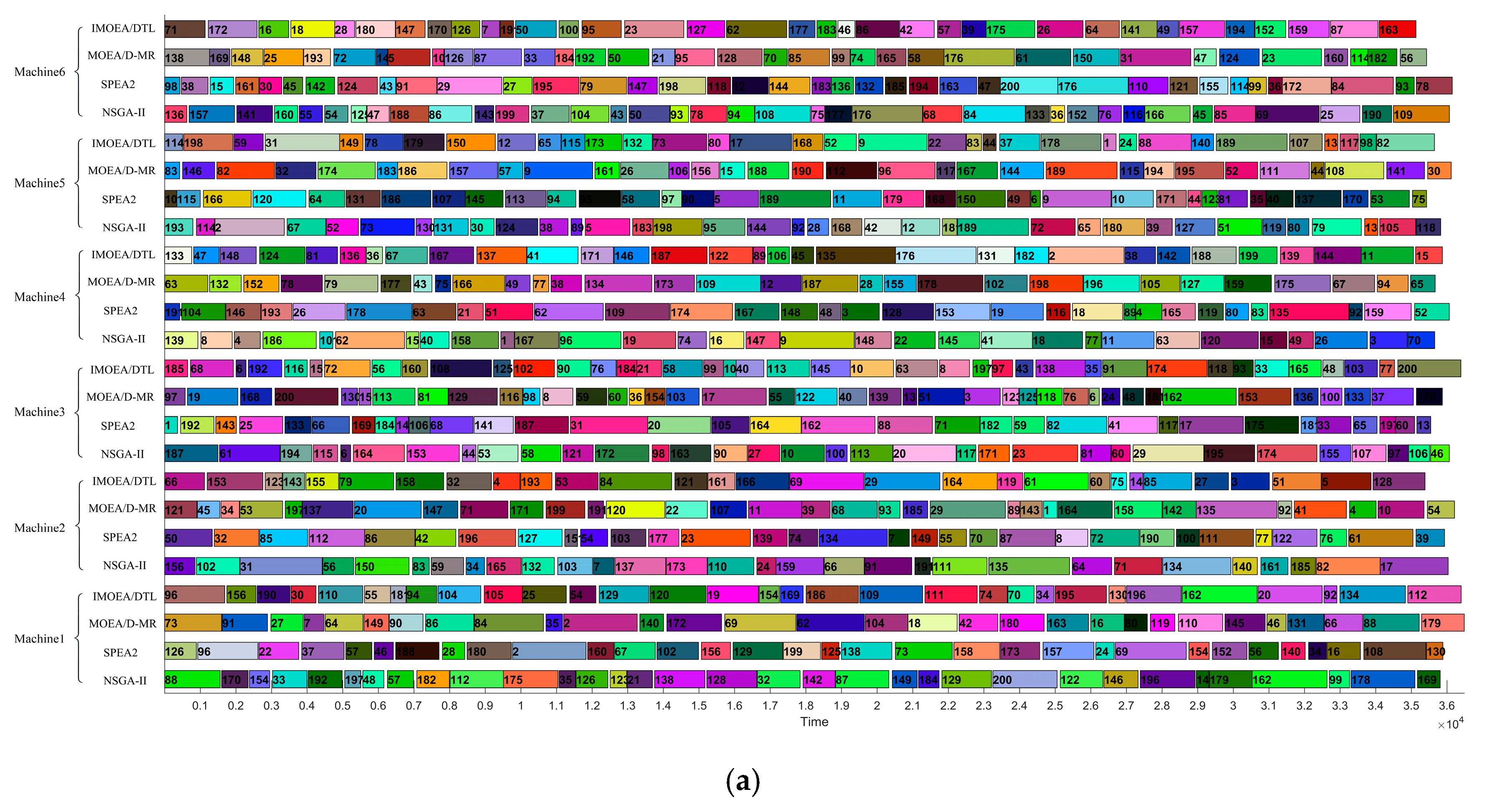
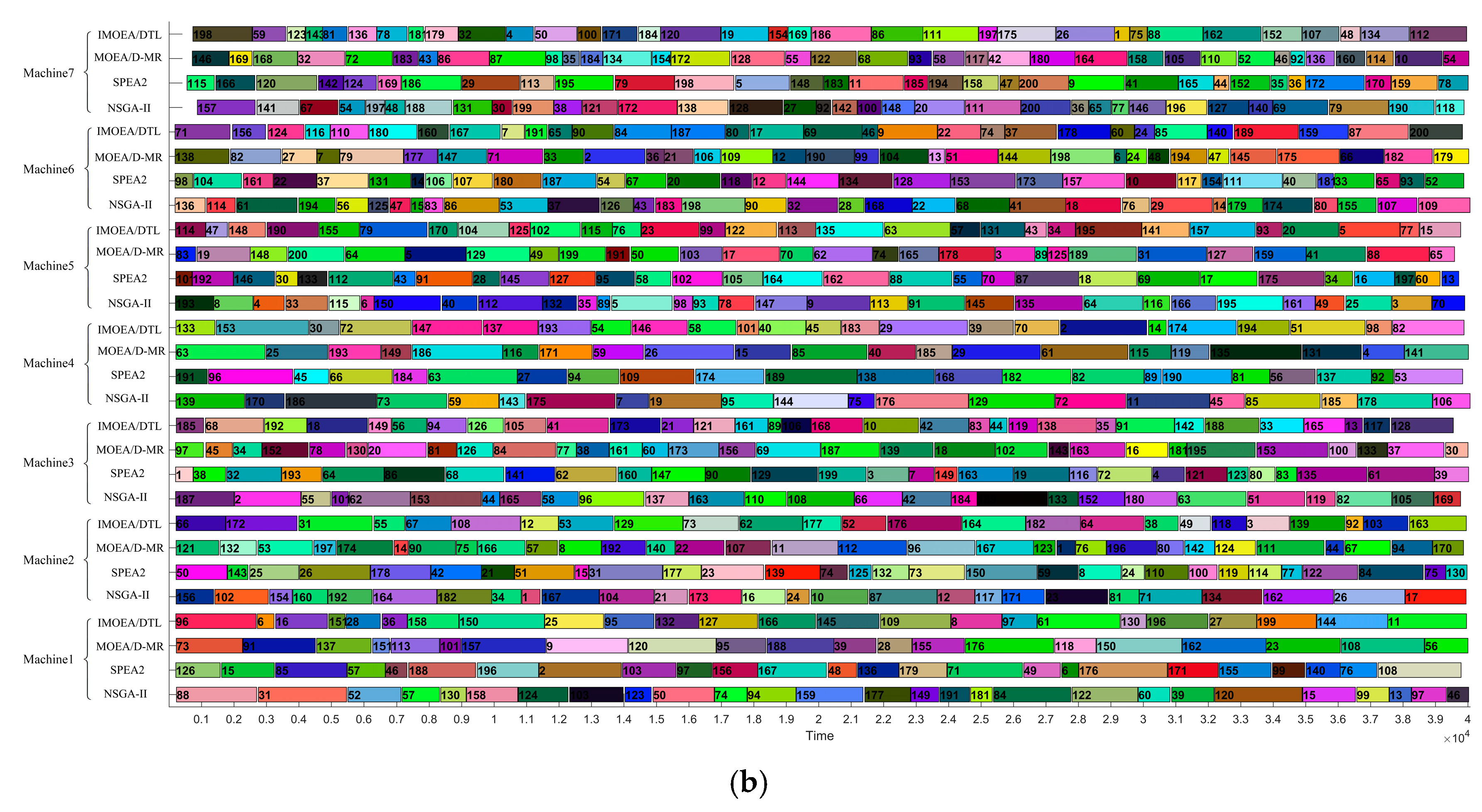
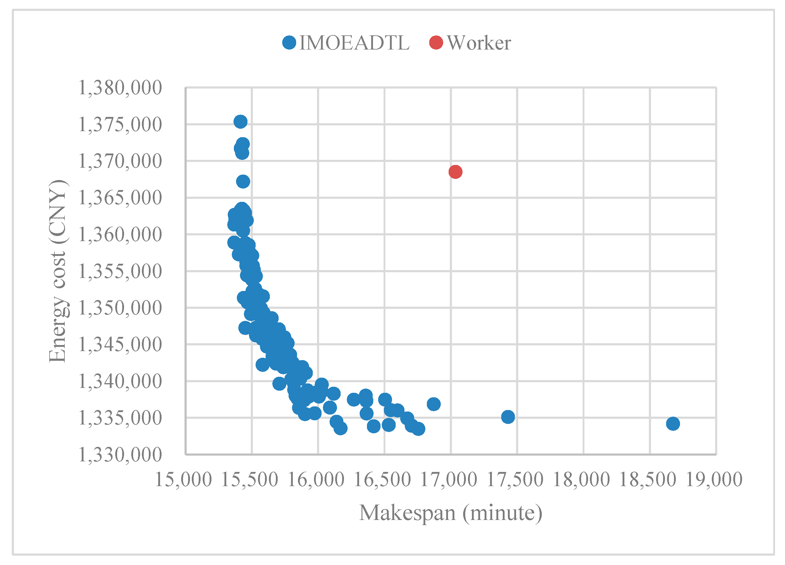
4.4. Results and Discussion

Table 8. C-metric of the solutions obtained by MOEA/D-MR, NSGA-II, SPEA2, and IMOEA/DTL.

Problems	$\mathit{C}\left(\mathit{W},\mathit{Z}\right)$	$\mathit{C}\left(\mathit{Z},\mathit{W}\right)$	$\mathit{C}\left(\mathit{X},\mathit{Z}\right)$	$\mathit{C}\left(\mathit{Z},\mathit{X}\right)$	$\mathit{C}\left(\mathit{Y},\mathit{Z}\right)$	$\mathit{C}\left(\mathit{Z},\mathit{Y}\right)$
Job1	0	1	0	0.98	0	1
Job2	0	1	0	1	0	1
Job3	0	1	0	1	0	1
Job4	0	1	0	1	0	1
Job5	0	1	0	1	0	1
Job6	0	1	0	1	0	1
Job7	0	1	0	1	0	1
Job8	0	1	0	1	0	1
Job9	0	1	0	1	0	1
Job10	0	1	0	1	0	1
Job11	0	1	0	1	0	1
Job12	0	1	0	1	0	1
Job13	0	1	0	1	0	1
Job14	0	1	0	1	0	0.98
Job15	0	1	0	1	0	1
Job16	0	1	0	1	0	1

describes the mean C-metric of the solutions obtained by IMOEA/DTL, MOEA/D-MR, SPEA2, and NSGA-II. W, X, Y, and Z represent the solutions obtained by MOEA/D-MR, NSGA-II, SPEA2, and IMOEA/DTL, respectively. From Table 8, it can be seen that $C\left(Z,W\right)$ is larger than $C\left(W,Z\right)$, $C\left(Z,X\right)$ is larger than $C\left(X,Z\right)$, and $C\left(Z,Y\right)$ is larger than $C\left(Y,Z\right)$ in 16 scheduling problems. The values of $C\left(Z,W\right), C\left(Z,X\right)$ and $C\left(Z,Y\right)$ are close to one in the eight scheduling problems. Meanwhile, the values of $C\left(W,Z\right), C\left(X,Z\right)$, and $C\left(Y,Z\right)$ are almost equal to zero. The C-metric indicates that other methods dominate the few solutions obtained by IMOEA/DTL. However, some solutions of IMOEA/DTL dominate all solutions obtained by MOEA/D-MR, NSGA-II, and SPEA2. As shown in Table 8, the solutions obtained by IMOEA/DTL have better performance than those obtained by MOEA/D-MR, NSGA-II, and SPEA2 in C-metric.

Table 9. The p-value of the Wilcoxon signed-rank test of the C-metric between two algorithms.

Problems	P1	P2	P3
Job1	0.0020	0.0020	0.0020
Job2	0.0020	0.0020	0.0020
Job3	0.0020	0.0020	0.0020
Job4	0.0020	0.0020	0.0020
Job5	0.0020	0.0020	0.0020
Job6	0.0020	0.0020	0.0020
Job7	0.0020	0.0020	0.0020
Job8	0.0020	0.0020	0.0020
Job9	0.0020	0.0020	0.0020
Job10	0.0020	0.0020	0.0020
Job11	0.0020	0.0020	0.0020
Job12	0.0020	0.0020	0.0020
Job13	0.0020	0.0020	0.0020
Job14	0.0020	0.0020	0.0020
Job15	0.0020	0.0020	0.0020
Job16	0.0020	0.0020	0.0020

shows the p-value in the Wilcoxon signed-rank test of the C-metric between two algorithms. P1 represents the p-value of the Wilcoxon signed-rank test of the C-metric between IMOEA/DTL and MOEA/D-MR, P2 represents the p-value of the Wilcoxon signed-rank test of the C-metric between IMOEA/DTL and NSGA-II, and P3 represents the p-value of the Wilcoxon signed-rank test of the C-metric between IMOEA/DTL and SPEA2. P1, P2, and P3 are less than 0.05 in 16 scheduling problems, indicating significant differences between IMOEA/DTL and MOEA/D-MR, IMOEA/DTL and NSGA-II, IMOEA/DTL and SPEA2. Table 8 and Table 9 indicate that IMOEA/DTL is superior to MOEA/D-MR, NSGA-II, and SPEA2 in terms of C-metric.

Table 10. Average values of hypervolume indicator (HV-metric) of the solutions obtained by MOEA/D-MR, NSGA-II, SPEA2, and IMOEA/DTL.

Problems	MOEA/D-MR	NSGA-II	SPEA2	IMOEA/DTL
Job1	3.46 × 107	3.32 × 107	3.42 × 107	5.43 × 107
Job2	1.75 × 107	1.65 × 107	1.58 × 107	2.79 × 107
Job3	7.02 × 107	6.38 × 107	6.60 × 107	9.82 × 107
Job4	5.33 × 107	5.04 × 107	5.15 × 107	8.27 × 107
Job5	3.33 × 107	3.06 × 107	3.09 × 107	4.92 × 107
Job6	3.40 × 107	3.53 × 107	3.37 × 107	5.87 × 107
Job7	4.22 × 107	3.74 × 107	4.03 × 107	6.29 × 107
Job8	2.40 × 107	2.01 × 107	2.07 × 107	3.65 × 107
Job9	5.99 × 107	5.44 × 107	5.75 × 107	8.79 × 107
Job10	2.66 × 107	2.62 × 107	2.60 × 107	4.32 × 107
Job11	4.41 × 107	4.49 × 107	4.45 × 107	7.30 × 107
Job12	4.43 × 107	4.07 × 107	4.18 × 107	6.58 × 107
Job13	5.43 × 107	5.43 × 107	5.46 × 107	8.77 × 107
Job14	3.32 × 107	3.27 × 107	3.35 × 107	5.16 × 107
Job15	4.83 × 107	4.54 × 107	4.62 × 107	7.67 × 107
Job16	8.19 × 107	7.78 × 107	8.15 × 107	1.19 × 107

lists the average value of HV-metric of the solutions obtained by IMOEA/DTL, MOEA/D-MR, SPEA2, and NSGA-II. The solutions obtained by IMOEA/DTL have a larger average HV-metric than those obtained by MOEA/D-MR, SPEA2, and NSGA-II in all scheduling problems, indicating that the proximity and diversity of the solutions of IMOEA/DTL are best in all solutions. As shown in Table 10, the solutions obtained by MOEA/D-MR, NSGA-II, and SPEA2 are inferior to that obtained by IMOEA/DTL in terms of HV-metric. The p-value of the Wilcoxon signed-rank test of the HV-metric between two algorithms is shown in

Table 11. The p-value of the Wilcoxon signed-rank test of the HV-metric between two algorithms.

Problems	P1	P2	P3
Job1	0.0020	0.0020	0.0020
Job2	0.0020	0.0020	0.0020
Job3	0.0020	0.0020	0.0020
Job4	0.0020	0.0020	0.0020
Job5	0.0020	0.0020	0.0020
Job6	0.0020	0.0020	0.0020
Job7	0.0020	0.0020	0.0020
Job8	0.0020	0.0020	0.0020
Job9	0.0020	0.0020	0.0020
Job10	0.0020	0.0020	0.0020
Job11	0.0020	0.0020	0.0020
Job12	0.0020	0.0020	0.0020
Job13	0.0020	0.0020	0.0020
Job14	0.0020	0.0020	0.0020
Job15	0.0020	0.0020	0.0020
Job16	0.0020	0.0020	0.0020

. P1 represents the p-value of the Wilcoxon signed-rank test of the HV-metric between IMOEA/DTL and MOEA/D-MR, P2 represents the p-value of the Wilcoxon signed-rank test of the HV-metric between IMOEA/DTL and NSGA-II, and P3 represents the p-value of the Wilcoxon signed-rank test of the HV-metric between IMOEA/DTL and SPEA2. P1, P2, and P3 are less than 0.05, demonstrating the significant differences between IMOEA/DTL and MOEA/D-MR, IMOEA/DTL and NSGA-II, and IMOEA/DTL and SPEA2. Table 10 and Table 11 indicate that IMOEA/DTL is superior to MOEA/D-MR, NSGA-II, and SPEA2 in terms of HV-metric.

In order to intuitively show the scheduling schemes obtained by different algorithms, some Gantt charts of scheduling schemes obtained by different algorithms are provided, as shown in Figure 4, Figure 5 and Figure 6. Each scheduling scheme corresponds to a solution in the Pareto front. We only provide Gantt charts of Job1, Job8, and Job16, and the Gantt charts for other scheduling problems are similar to these three. In the Gantt charts below, we can see how the jobs are organized and processed for the scheduling scheme obtained by each algorithm, and it can be seen that the scheduling scheme obtained by IMOEA/DTL has a smaller makespan. Not only that, in all the following scheduling schemes, IMOEA/DTL has the smallest energy cost.

Table 12. The average makespan and average energy cost obtained by MOEA/D-MR, NSGA-II, SPEA2, and IMOEA/DTL.

Problems	Makespan (Minute)				Energy Cost (CNY)
	MOEA/D-MR	NSGA-II	SPEA2	IMOEA/DTL	MOEA/D-MR	NSGA-II	SPEA2	IMOEA/DTL
Job1	10,049	10,064	10,053	9939	801,309	803,965	804,358	795,656
Job2	11,817	11,864	11,881	11,800	964,677	966,456	966,000	957,500
Job3	14,104	14,139	14,175	14,033	1,158,100	1,161,747	1,159,518	1,150,038
Job4	16,030	16,089	16,128	16,008	1,302,626	1,304,014	1,303,485	1,291,973
Job5	18,534	18,537	18,567	18,460	1,520,818	1,521,966	1,521,371	1,511,605
Job6	19,603	19,680	19,642	19,531	1,610,892	1,608,901	1,610,826	1,596,377
Job7	21,236	21,348	21,337	21,222	1,777,566	1,779,676	1,778,261	1,768,963
Job8	23,006	23,044	23,063	22,953	1,916,511	1,921,468	1,918,722	1,908,951
Job9	27,008	27,075	27,079	26,922	2,223,799	2,226,399	2,224,613	2,213,336
Job10	26,571	26,585	26,584	26,501	2,193,870	2,193,213	2,193,967	2,183,339
Job11	28,920	28,914	29,001	28,886	2,427,444	2,426,101	2,424,184	2,408,955
Job12	30,127	30,167	30,219	30,117	2,565,900	2,568,756	2,566,343	2,551,189
Job13	32,440	32,451	32,510	32,358	2,699,366	2,700,491	2,697,074	2,684,005
Job14	35,034	35,093	35,078	34,972	2,887,249	2,887,706	2,886,665	2,876,694
Job15	35,787	35,835	35,768	35,712	2,984,084	2,985,389	2,985,440	2,971,161
Job16	40,290	40,241	40,253	40,185	3,380,449	3,385,432	3,383,498	3,368,202

shows the average makespan and average energy cost obtained by MOEA/D-MR, NSGA-II, SPEA2, and IMOEA/DTL. Table 12 indicates that both the average makespan and average energy cost obtained by IMOEA/DTL are lower than those obtained by MOEA/D-MR, NSGA-II, and SPEA2. Therefore, IMOEA/DTL can provide the solution with lower makespan and energy cost than MOEA/D-MR, NSGA-II, and SPEA2. This study adopts a multi-objective algorithm, and a non-dominated solution set is obtained. The solutions in the non-dominated solution set have lower energy cost or makespan, but they are mutually exclusive. Decision makers can select an optimal solution on the basis of actual situations. For instance, the solution with a low makespan can be selected in the case of a heavy production task, which can improve the utilization efficiency of the workshop and ensure that the task can be completed on schedule. On the contrary, the decision-makers can choose the optimal solution with low energy cost to reduce the production cost.

In China, most of the scheduling jobs of the tissue paper mills are completed by workers based on their experience. The quality of the scheduling depends on the experience of the workers. In this study, a real scheduling problem is solved by IMOEA/DTL, and the solution is compared with that obtained by workers. The solution obtained by workers has the makespan of 17,035 and the energy cost of 1,368,497.

Table 13. The average, maximum, and minimum value of energy cost and makespan obtained by IMOEA/DTL.

Average Makespan (Minute)	Average Energy cost (CNY)	Maximum Makespan (Minute)	Minimum Energy Cost (CNY)	Minimum Makespan (Minute)	Maximum Energy Cost (CNY)
15,754	1,347,737	18,675	1,333,494	15,367	1,375,361

indicates that the average makespan obtained by IMOEA/DTL is about 7.5% less than that obtained by the worker. The average energy cost obtained by IMOEA/DTL is about 1.5% less than that obtained by the worker. From Table 13, it can be seen that the minimum energy cost is 1,333,494, and the corresponding makespan is 16,754, which reduces by 2.6% and 1.6%, respectively. The minimum makespan is 15,367, and the corresponding energy cost is 1,361,331, which decrease by 9.8% and 0.5%, respectively. The largest energy cost is 1,375,361, which is 0.5% higher than the cost obtained by the worker, but the corresponding makespan is reduced by 9.5%. The largest makespan is 18,675, which is 8.8% higher than the cost obtained by the worker, but the corresponding energy cost is reduced by 2.5%. It can be concluded that IMOEA/DTL can reduce both the energy cost and the makespan. Although the maximum makespan and the maximum energy cost are larger than those obtained by the worker, the corresponding energy cost and makespan are smaller. Figure 7 shows the scatter plot for the solutions obtained by IMOEA/DTL and the worker. The energy cost obtained by IMOEA/DTL is lower than that obtained by the worker. The solutions of IMOEA/DTL with lower energy cost than that obtained by the worker account for about 98.56% of the total solutions of IMOEA/DTL. While the solutions of IMOEA/DTL with lower makespan than that obtained by the worker account for about 97.12% of the total solutions of IMOEA/DTL. About 95.68% of the total solutions obtained by IMOEA/DTL have lower energy cost and makespan than those obtained by the worker.

In practical applications, the construction of basic data is a particularly critical issue, especially setup-related data, which requires a lot of statistical data. We suggest that a part of the key data can be constructed through the manufacturing execution system, and through the manufacturing execution system, we can know the status of machine, personnel, and materials in real time, and thus make timely responses to emergencies in the production process. In addition, we recommend using commercial production scheduling software and then integrating the model into commercial software. Compared with developing a scheduling system from scratch, this has a higher success rate.

5. Conclusions

This study explored a novel energy-saving approach by scheduling under TOU electricity tariffs for tissue paper mills. First of all, an energy cost model was established based on TOU electricity tariffs. The energy cost consists of transportation energy cost, set-up energy cost, and processing energy cost. Second, an energy-efficiency scheduling model was built on the basis of the scheduling model and the energy cost model. Finally, the model was solved by proposing a novel IMOEA/DTL method. The experiment made a comparison between the proposed method and two popular multi-objective optimization methods, MOEA/D-MR, NSGA-II, and SPEA2. The experiment results demonstrate that the proposed method performs better than NSGA-II and SPEA2 in terms of C-metric and HV-metric. Moreover, the proposed method has been proven to have an energy-saving ratio of 2.6% through a real scheduling problem. Considering the similarity between the production processes in tissue paper mills and other papermaking mills, the results are of great reference significance for other papermaking mills.

However, this study implemented the algorithms by MATLAB, and the speed of the algorithms should be further improved. Therefore, the speed of the algorithms will be improved in future research.

References

1. EIA. Available online: https://www.eia.gov/outlooks/aeo/data/browser/#/?id=37-AEO2020&cases=ref2020&sourcekey=1 (accessed on 22 December 2020).
2. EIA. Available online: https://www.eia.gov/outlooks/aeo/data/browser/#/?id=22-AEO2020&cases=ref2020&sourcekey=0 (accessed on 22 December 2020).
3. Mouzon, G.; Yildirim, M.B. A framework to minimise total energy consumption and total tardiness on a single machine. Int. J. Sustain. Eng. 2008, 1, 105–116. [Google Scholar] [CrossRef]
4. Che, A.; Wu, X.; Peng, J.; Yan, P. Energy-efficient bi-objective single-machine scheduling with power-down mechanism. Comput. Oper. Res. 2017, 85, 172–183. [Google Scholar] [CrossRef]
5. Lu, C.; Gao, L.; Li, X.; Pan, Q.; Wang, Q. Energy-efficient permutation flow shop scheduling problem using a hybrid multi-objective backtracking search algorithm. J. Clean. Prod. 2017, 144, 228–238. [Google Scholar] [CrossRef]
6. Mokhtari, H.; Hasani, A. An energy-efficient multi-objective optimization for flexible job-shop scheduling problem. Comput. Chem. Eng. 2017, 104, 339–352. [Google Scholar] [CrossRef]
7. Nolde, K.; Morari, M. Electrical load tracking scheduling of a steel plant. Comput. Chem. Eng. 2010, 34, 1899–1903. [Google Scholar] [CrossRef] [Green Version]
8. Wu, N.; Li, Z.; Qu, T. Energy efficiency optimization in scheduling crude oil operations of refinery based on linear programming. J. Clean. Prod. 2017, 166, 49–57. [Google Scholar] [CrossRef]
9. Wu, X.L.; Sun, Y.L. A green scheduling algorithm for flexible job shop with energy-saving measures. J. Clean. Prod. 2018, 172, 3249–3264. [Google Scholar] [CrossRef]
10. Che, A.; Zhang, S.; Wu, X. Energy-conscious unrelated parallel machine scheduling under time-of-use electricity tariffs. J. Clean. Prod. 2017, 156, 688–697. [Google Scholar] [CrossRef]
11. Cheng, J.; Chu, F.; Liu, M.; Wu, P.; Xia, W. Bi-criteria single-machine batch scheduling with machine on/off switching under time-of-use tariffs. Comput. Int. Eng. 2017, 112, 721–734. [Google Scholar] [CrossRef]
12. Lee, S.; Chung, B.D.; Jeon, H.W.; Chang, J. A dynamic control approach for energy-efficient production scheduling on a single machine under time-varying electricity pricing. J. Clean. Prod. 2017, 165, 552–563. [Google Scholar] [CrossRef]
13. Zhou, S.; Li, X.; Du, N.; Pang, Y.; Chen, H. A multi-objective differential evolution algorithm for parallel batch processing machine scheduling considering electricity consumption cost. Comput. Oper. Res. 2018, 96, 55–68. [Google Scholar] [CrossRef]
14. Gong, X.; De Pessemier, T.; Martens, L.; Joseph, W. Energy- and labor-aware flexible job shop scheduling under dynamic electricity pricing: A many-objective optimization investigation. J. Clean. Prod. 2019, 209, 1078–1094. [Google Scholar] [CrossRef] [Green Version]
15. Luo, H.; Du, B.; Huang, G.Q.; Chen, H.; Li, X. Hybrid flow shop scheduling considering machine electricity consumption cost. Int. J. Prod. Econ. 2013, 146, 423–439. [Google Scholar] [CrossRef]
16. Zhang, H.; Zhao, F.; Fang, K.; Sutherland, J.W. Energy-conscious flow shop scheduling under time-of-use electricity tariffs. CIRP Ann. Manuf. Technol. 2014, 63, 37–40. [Google Scholar] [CrossRef]
17. Pan, R.L.; Li, Z.H.; Gao, J.H.; Zhang, H.L.; Xia, X. Electrical load tracking scheduling of steel plants under time-of-use tariffs. Comput. Int. Eng. 2019, 137, 106049. [Google Scholar] [CrossRef]
18. Sharma, A.; Zhao, F.; Sutherland, J.W. Econological scheduling of a manufacturing enterprise operating under a time-of-use electricity tariff. J. Clean. Prod. 2015, 108, 256–270. [Google Scholar] [CrossRef]
19. Tan, Y.; Liu, S. Models and optimisation approaches for scheduling steelmaking–refining–continuous casting production under variable electricity price. Int. J. Prod. Res. 2014, 52, 1032–1049. [Google Scholar] [CrossRef]
20. Zeng, Y.J.; Sun, Y.G. Short-term scheduling of steam power system in iron and steel industry under time-of-use power price. J. Iron. Steel. Res. Int. 2015, 22, 795–803. [Google Scholar] [CrossRef]
21. Zhao, X.; Bai, H.; Shi, Q.; Lu, X.; Zhang, Z. Optimal scheduling of a byproduct gas system in a steel plant considering time-of-use electricity pricing. Appl. Energy 2017, 195, 100–113. [Google Scholar] [CrossRef]
22. Ramos, A.G.; Leal, J. ILP model for energy-efficient production scheduling of flake ice units in food retail stores. J. Clean. Prod. 2017, 156, 953–961. [Google Scholar] [CrossRef]
23. Yan, J.; Li, L.; Zhao, F.; Zhang, F.; Zhao, Q. A multi-level optimization approach for energy-efficient flexible flow shop scheduling. J. Clean. Prod. 2016, 137, 1543–1552. [Google Scholar] [CrossRef]
24. Fang, K.; Uhan, N.A.; Zhao, F. Scheduling on a single machine under time-of-use electricity tariffs. Ann. Oper. Res. 2016, 238, 199–227. [Google Scholar] [CrossRef]
25. Tan, M.; Duan, B.; Su, Y. Economic batch sizing and scheduling on parallel machines under time-of-use electricity pricing. Oper. Res. Ger. 2016, 18, 105–122. [Google Scholar] [CrossRef]
26. Zeng, Z.Q.; Hong, M.N.; Man, Y.; Li, J.G.; Zhang, Y.Z.; Liu, H.B. Multi-object optimization of flexible flow shop scheduling with batch process—Consideration total electricity consumption and material wastage. J. Clean. Prod. 2018, 183, 925–939. [Google Scholar] [CrossRef]
27. Zeng, Z.Q.; Hong, M.N.; Li, J.G.; Man, Y.; Liu, H.B.; Li, Z.; Zhang, H.H. Integrating process optimization with energy-efficiency scheduling to save energy for paper mills. Appl. Energ. 2018, 225, 542–558. [Google Scholar] [CrossRef]
28. Zhang, Q.; Li, H. MOEA/D: A multiobjective evolutionary algorithm based on decomposition. IEEE Trans. Evolut. Comput. 2007, 11, 712–731. [Google Scholar] [CrossRef]
29. Adasme, P.; Lisser, A. Uplink scheduling for joint wireless orthogonal frequency and time division multiple access networks. J. Sched. 2016, 19, 349–366. [Google Scholar] [CrossRef]
30. Anjana, V.; Sridharan, R.; Kumar, P.N.R. Metaheuristics for solving a multi-objective flow shop scheduling problem with sequence-dependent setup times. J. Sched. 2019, 23, 49–69. [Google Scholar] [CrossRef]
31. Wang, Z.; Zhang, Q.; Li, H.; Ishibuchi, H.; Jiao, L. On the use of two reference points in decomposition based multiobjective evolutionary algorithms. Swarm. Evol. Comput. 2017, 34, 89–102. [Google Scholar] [CrossRef] [Green Version]
32. Schulz, S.; Neufeld, J.S.; Buscher, U. A multi-objective iterated local search algorithm for comprehensive energy-aware hybrid flow shop scheduling. J. Clean. Prod. 2019, 224, 421–434. [Google Scholar] [CrossRef]
33. Kantour, N.; Bouroubi, S.; Chaabane, D. A parallel MOEA with criterion-based selection applied to the Knapsack Problem. Appl. Soft Comput. 2019, 80, 358–373. [Google Scholar] [CrossRef] [Green Version]
34. Zhang, R.; Chiong, R. Solving the energy-efficient job shop scheduling problem: A multiobjective genetic algorithm with enhanced local search for minimizing the total weighted tardiness and total energy consumption. J. Clean. Prod. 2016, 112, 3361–3375. [Google Scholar] [CrossRef]
35. Li, M.; Lei, D.; Cai, J. Two-level imperialist competitive algorithm for energy-efficient hybrid flow shop scheduling problem with relative importance of objectives. Swarm. Evol. Comput. 2019, 49, 34–43. [Google Scholar] [CrossRef]
Figure 1. Production process of tissue paper mills.
Processes 09 00274 g001
Figure 2. The flow chart of Multi-Objective Evolutionary Algorithm based on Decomposition (MOEA/D).
Processes 09 00274 g002
Figure 3. The flow chart of Multi-Objective Evolutionary Algorithm based on Decomposition and Teaching–Learning-Based Optimization (MOEA/DTL).
Processes 09 00274 g003
Figure 4. The Gantt charts of Job1, (a,b) are Gantt charts of the first and second operation of Job1, respectively; the makespan and energy cost of NSGA-II, SPEA2, MOEA/D-MR, and IMOEA/DTL are (9.9020 × 10³, 8.1231 × 10⁵), (9.8583 × 10³, 8.1278 × 10⁵), (9.8063 × 10³, 8.1155 × 10⁵), and (9.6900 × 10³, 8.1150 × 10⁵) respectively.
Processes 09 00274 g004aProcesses 09 00274 g004b
Figure 5. The Gantt charts of Job8, (a,b) are Gantt charts of the first and second operation of Job8 respectively; the makespan and energy cost of NSGA-II, SPEA2, MOEA/D-MR, and IMOEA/DTL are (2.3041 × 10⁴, 1.9083 × 10⁶), (2.3147 × 10⁴, 1.9133 × 10⁶), (2.3112 × 10⁴, 1.9117 × 10⁶), and (2.3017 × 10⁴, 1.9041 × 10⁶), respectively.
Processes 09 00274 g005aProcesses 09 00274 g005b
Figure 6. The Gantt charts of Job16, (a,b) are Gantt charts of the first and second operation of Job16 respectively; the makespan and energy cost of NSGA-II, SPEA2, MOEA/D-MR, and IMOEA/DTL are (4.0066× 10⁴, 3.3994× 10⁶), (4.0020× 10⁴, 3.3900× 10⁶), (4.0029× 10⁴, 3.4038× 10⁶), and (3.9960× 10⁴, 3.3800× 10⁶) respectively.
Processes 09 00274 g006aProcesses 09 00274 g006b
Figure 7. The scatter plot for the solutions obtained by IMOEA/DTL and a worker.
Processes 09 00274 g007