Matching Optimization of a Mixed Flow Pump Impeller and Diffuser Based on the Inverse Design Method

Abstract

When considering the interaction between the impeller and diffuser, it is necessary to provide logical and systematic guidance for their matching optimization. In this study, the goal was to develop a comprehensive matching optimization strategy to optimize the impeller and diffuser of a mixed flow pump. Some useful tools and methods, such as the inverse design method, computational fluid dynamics (CFD), design of experiment, surrogate model, and optimization algorithm, were used. The matching optimization process was divided into two steps. In the first step, only the impeller was optimized. Thereafter, CFD analysis was performed on the optimized impeller to get the circulation and flow field distribution at the outlet of the impeller. In the second step of optimization, the flow field and circulation distribution at the inlet of the diffuser were set to be the same as the optimized impeller outlet. The results show that the matching optimization strategy proposed in this study is effective and can overcome the shortcomings of single-component optimization, thereby further improving the overall optimization effect. Compared with the baseline model, the pump efficiency of the optimized model at 1.2Q_des, 1.0Q_des, and 0.8Q_des is increased by 6.47%, 3.68%, and 0.82%, respectively.

1. Introduction

As one of the most important machines in modern civilization, the performance of rotating machinery will have a great influence on the development of wider society. Published data in the Annual Work Report of the Chinese Government in 2019 revealed that more than 98% of the country’s electric power conversion is done by rotating machinery. Consequently, a marginal increase in the efficiency of rotating machinery will produce unimaginable economic benefits. For instance, in China, for every 1% increase in rotating machinery efficiency, about 70 billion kilowatts of electricity can be saved annually. As a kind of rotating machinery, mixed flow pumps play an important role in industrial production, agricultural irrigation, and urban drainage due to their moderate head, wide high efficiency range, and good anti-cavitation performance. Thus, it is of great significance to study the optimization design of mixed flow pumps.

In the field of rotating machinery optimization, computational fluid dynamics (CFD) prediction is a better method than experimental investigation, because the former is more convenient and cheaper [1]. More importantly, CFD prediction can provide flow details inside the rotating machinery, which can help designers better understand the reasons for performance changes and make targeted optimization [2]. However, CFD prediction cannot directly provide the optimal solution for the optimization of rotating machinery. Like most complex optimization problems, the optimization of rotating machinery usually entails multiple indicators, and each target affects the other. Therefore, considering the multi-objectivity of the rotating machinery optimization is inevitable [3]. Several attempts have been made to solve the above problem. Eventually, the method of combined optimization strategy consisting of CFD, design of experiment (DOE), surrogate models, and optimization algorithms came to the fore and achieved satisfactory results. Meng et al. [4] combined CFD, Latin hypercube sampling (LHS), a two-layer artificial neural network (ANN), and a non-dominated sorting genetic algorithm (NSGA) to successfully improve the reverse operation performance of the axial flow pump without reducing the forward flow performance. Shi et al. [5] applied LHS, the response surface method (RSM), and an adaptive mutation probability genetic algorithm (AMGA) to the multi-disciplinary optimization of the axial flow pump. This effectively reduced the weight of the blade and enhanced its hydraulic efficiency on the premise of meeting the requirements of blade strength. Pei et al. [6] and Wang et al. [7] used LHS, ANN and modified particle swarm optimization (MPSO) to optimize the impeller and diffuser of a centrifugal pump, and widen the high efficiency area. Shim et al. [8] optimized the efficiency, cavitation, and stability of a centrifugal pump by combined usage of LHS, kriging model, and NSGA. Kim et al. [9] studied the influence of hub ratio on the performance of the mixed flow pump at the same specific speed through the combined optimization strategy. Suh et al. [10] combined central composite design (CCD), RSM, and sequence quadratic program (SQP) to improve the efficiency and cavitation performance of mixed flow pumps at the design point.

In the above optimization, the parameterization of the impeller is completed by geometric parameters. With the development of computational fluid dynamics, the use of hydrodynamic parameters to parameterize the impeller has shown great potential. This technique is also known as the inverse design method (IDM). In IDM, the blade shape is controlled by blade loading, circulation, and stacking condition. Compared with the former, the latter requires fewer design parameters and has a closer relationship between design parameters and hydraulic performance [11]. Goto et al. [12] and Zangeneh et al. [13] ascertained the efficacy of IDM in mixed flow pump design by simulation and experiment. Huang et al. [14] improved the head and efficiency of the mixed flow pump at design point by using IDM, LHS, radial basis neural network (RBNN), and NSGA. Yiu et al. [15] increased the mixed flow pump efficiency and suction performance by combined usage of IDM and a genetic algorithm (GA). Zhu et al. [16] optimized the pressure distribution of the compressor through IDM, GA, and adjoint method, thus expanding its high efficiency area. The efficiency, stability, and cavitation performance of pump as turbine were improved by combining the use of IDM, DOE, RSM/RBNN, and NSGA [17,18,19,20].

There is a common point in the above studies, which is only the impeller or diffuser was optimized in each study, and the interaction between the two was ignored. Only a few kinds of research have studied the matching optimization of impeller and diffuser. Bonaiuti et al. [21] studied the simultaneous optimization of compressor impeller and diffuser through five loading parameters. Subsequently, in another work [22], by optimizing the diffuser first and then the impeller, the matching optimization of a waterjet pump diffuser and impeller was studied by the trial-and-error method. Yang et al. [23] investigated the influence of blade loading on the impeller and diffuser of the submersible axial-flow pump. However, due to the particularity of IDM, there are still some defects in these matching optimization studies. In IDM, the flow field and circulation distribution at the diffuser inlet are two important input parameters. To reduce the hydraulic losses, the flow field and circulation distribution at the diffuser inlet should be set to be the same as the impeller outlet [24]. Therefore, in the matching optimization of impeller and diffuser, the impeller should be optimized before the diffuser was optimized.

This study aims to provide systematic guidance for the matching optimization of a mixed flow pump impeller and diffuser based on IDM. Firstly, the mixed flow pump design specification and matching optimization strategy were introduced, and the accuracy of the CFD analysis was verified. Then, the strategy was applied to the matching optimization of the impeller and diffuser, and the key points of matching optimization were introduced. Finally, the optimization mechanism was clarified by a comparative analysis of the internal flow field of the two models.

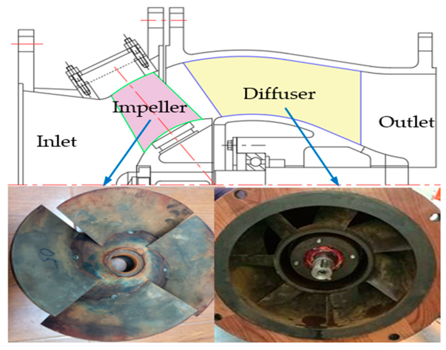
2. Mixed Flow Pump Model

The mixed flow pump as shown in Figure 1 was selected as the baseline model, which consists of an outlet elbow, a seven-blade diffuser, a four-blade impeller and a straight inlet pipe. The design flow rate Q_des is 0.4207 m³/s, the design head $H_{des}$ is 12.66 m, the rotational speed $N$ of the impeller is 1450 r/min, and the specific speed $n_s$ can be calculated by Equation (1):

$$n_{\mathrm{s}}=\frac{3.65N\sqrt{Q_{\mathrm{des}}}}{H^{0.75}}$$

(1)

The performance of the baseline model was tested by Tianjin experimental bench, China. On the test bench, an intelligent differential pressure transmitter and intelligent torque speed sensor are used to measure head and torque, respectively. These devices yielded measurement errors of <±0.1%. Also, an intelligent electromagnetic flowmeter is used to measure flow rate, and the measurement errors is <±0.2%. The random uncertainty and overall uncertainty of this test bench are less than 0.1% and 0.3%, respectively. The test results shown in Figure 2 show that the efficiency of the baseline model at the design point is 86.3%. In this figure, $Q^{*}=Q/Q_{\mathrm{des}}$ is the normalized flow rate, and $H^{*}=H/H_{\mathrm{des}}$ is the normalized head. (The same dimensionless method was used in other parts of this paper.)

3. Optimization Strategy

As shown in Figure 3, the optimization system was built by combining the IDM, CFD, optimal Latin hypercube sampling (OLHS), RSM, Multi-island genetic algorithm (MIGA) and NSGA-Ⅱ. The entire optimization process was divided into two steps. In the first step of optimization, only the impeller was optimized, and the objective function was set as the impeller weighted efficiency at 1.2Q_des, 1.0Q_des and 0.8Q_des. Thereafter, CFD analysis was performed on the optimized impeller to get the circulation and flow field distribution at the outlet of the optimized impeller. In the second step of optimization, the diffuser was optimized, and the objective functions were the levels of pump efficiency at 1.2Q_des, 1.0Q_des and 0.8Q_des. To improve the optimization effect of this step, the flow field and circulation distribution at the inlet of the diffuser were set to be the same as the optimized impeller outlet.

3.1. 3D Inverse Design Method

The parameterization of the impeller is done by the inverse design software TURBOdesign 6.4 developed by Advanced Design Technology. In this procedure, we assume that the fluid is steady, inviscid and uniform, so that the only vorticity is the bound vorticity on the blades, and its strength was determined by a specified distribution of circumferentially averaged swirl velocity $r\overline{V_{\theta }}$ (directly related to the bound circulation $2\pi r\overline{V_{\theta }}$) [11,25]:

$$r\overline{V_{\theta }}=\frac{B}{2\mathsf{\pi }}{\displaystyle {\int }_0^{\frac{2\mathsf{\pi }}{B}}r{V}_{\theta }\mathrm{d}\theta }$$

(2)

Here, $r\overline{V_{\theta }}$, $B$, and $r$ are the circumferentially averaged velocity, blade numbers, and radius, respectively.

When the meridional shape and the distribution of $r\overline{V_{\theta }}$ are given, the pressure field in the blade passage can be calculated by the meridional derivation of circulation $\partial \left(r\overline{V_{\theta }}\right)/\partial m$:

$$p^{+}-p^{-}=\frac{2\mathsf{\pi }}{B}\rho \overline{W_{\mathrm{m}}}\frac{\partial r\overline{V_{\mathsf{\theta }}}}{\partial m}$$

(3)

Here, $p^{+}-p^{-}$, $\rho$, $m$, and $\overline{W_{\mathrm{m}}}$ are pressure difference across the blade, fluid density, normalized streamline on the meridional shape, and pitch-wise averaged relative velocity, respectively.

The blade shape can be calculated by the following equation:

$$(\overline{V_z}+v_{zbl})\frac{\partial f}{\partial z}+(\overline{V_r}+v_{rbl})\frac{\partial f}{\partial r}=\frac{r\overline{V_{\theta }}}{r^2}+\frac{v_{\theta bl}}{r}-\omega$$

(4)

Here, $v$ and $\overline{V}$ are the periodic velocity and circumferential average velocity, respectively, and subscripts $r$ and $z$ represent the radial and axial components of velocity, respectively. $f$ is the blade wrap angle that is $\theta$ value at the blade between the leading edge and trailing edge.

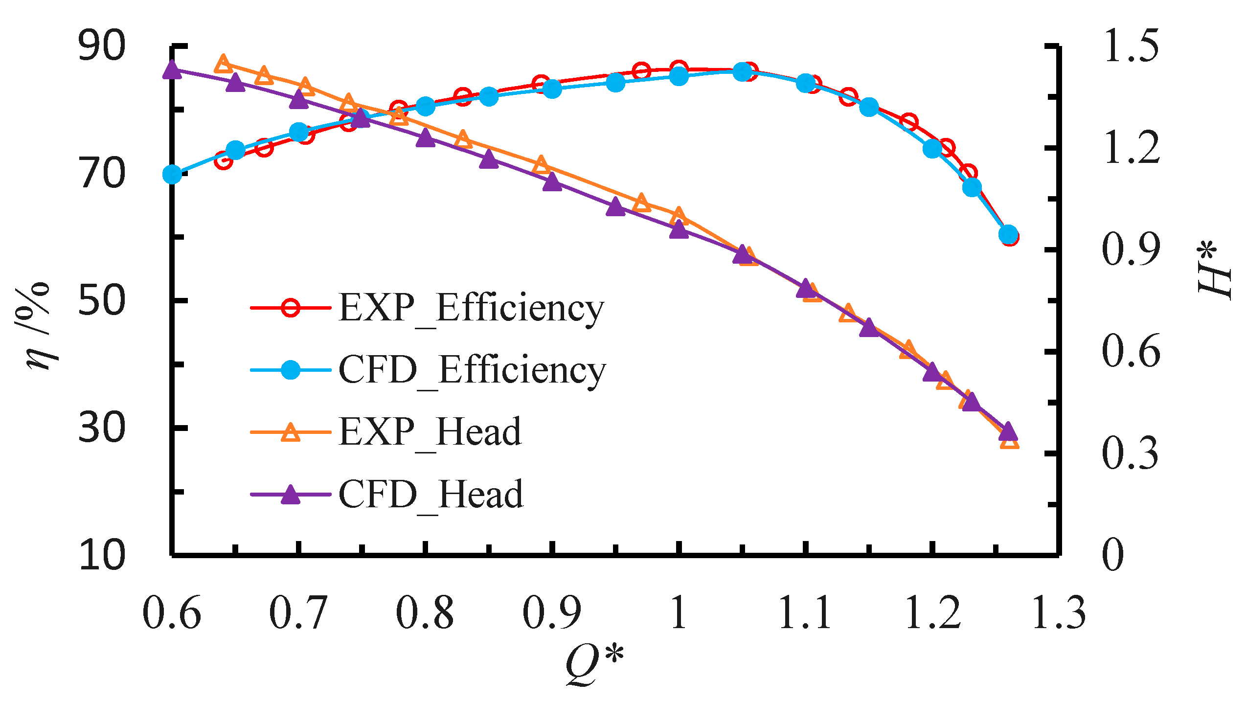
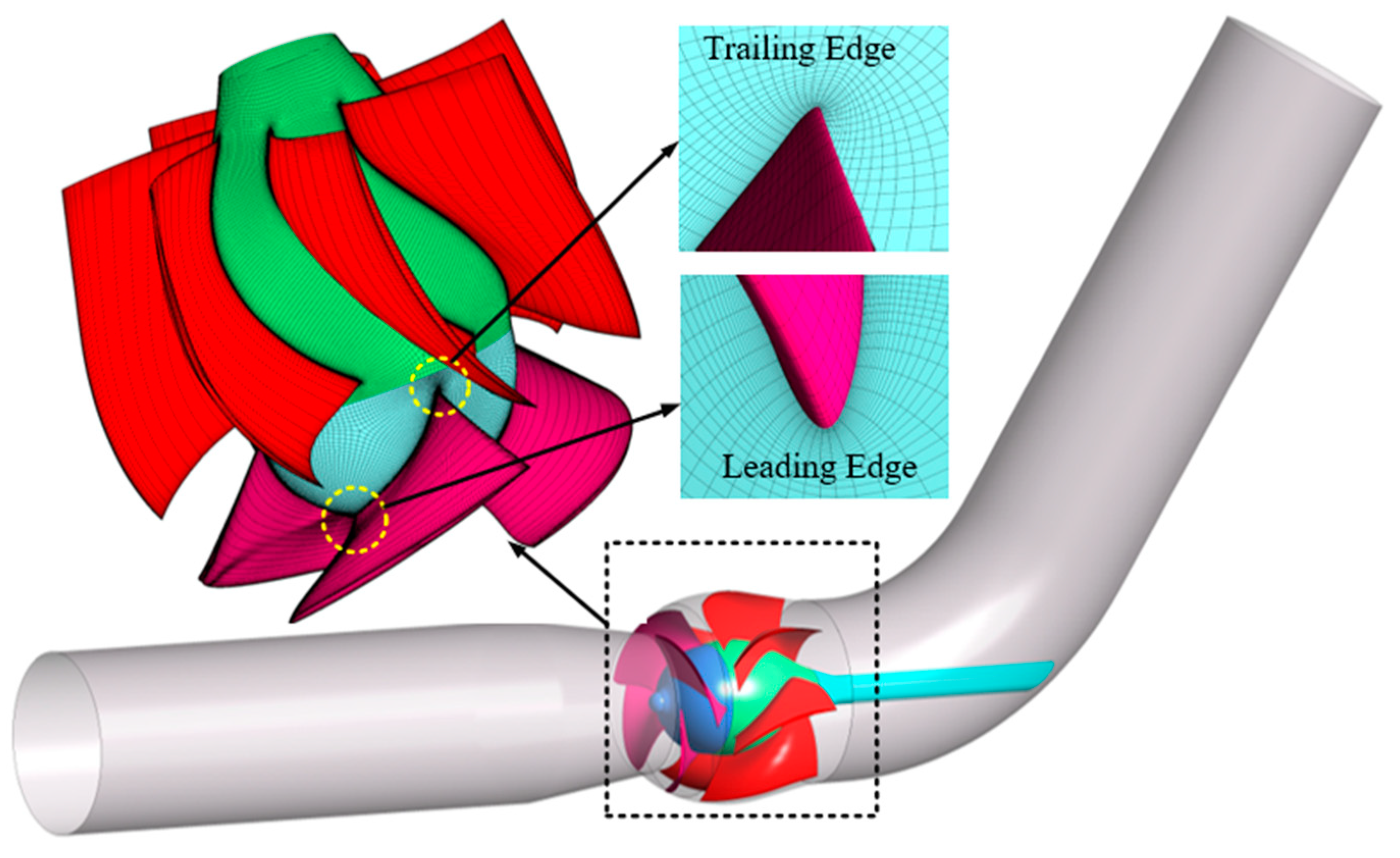
3.2. CFD Analyses and Validation

In this study, CFD analyses have the following three functions: one is to calculate the objective functions, the other is to analyze the flow field distribution of the optimized impeller and provide inlet flow field information for diffuser optimization, and the third is to verify the final optimization results. Therefore, the accuracy of CFD analyses is critical to the reliability of this work.

Thus, 3D steady incompressible Reynolds-Averaged Navier–Stokes ($\mathrm{RANS}$) equation was used in the full-passage simulation of the mixed flow pump. The $\mathrm{RANS}$ equation was solved by the shear stress transport $k-\omega$ turbulence model, because this model has the advantage of accurately calculating the internal flow pattern of the mixed flow pump [26]. A high-resolution scheme was selected to discretize the convective-diffusion terms [27]. The mass flow rate was set at the inlet, and the static pressure was set at the outlet. The frozen rotor frame of reference was adopted at the interface between the stationary and rotating domains. The convergence criteria were set to $5\times {10}^{-5}$.

The discretization of the computational domain is the basis of CFD analysis. In this study, the discretization of the computational domain is completed by structured grids, which have the advantages of controllable quality and quantity compared to unstructured grids. Mesh refinement was performed to all walls to ensure a small Y+ near the wall, O-type grids were used near the blade surface, and H/C-type grids were used near the blade edge. The meshing of the entire computational domain was completed by hexahedral grids as shown in Figure 4.

Table 1. Mesh independence analysis.

Inlet Pipe $\left(\times {10}^5\right)$	Impeller $\left(\times {10}^5\right)$	Diffuser $\left(\times {10}^5\right)$	Outlet Pipe $\left(\times {10}^5\right)$	Total Number $\left(\times {10}^5\right)$	Head (m)	Efficiency (%)
43	63	70	58	234	12.13	84.52
83	121	130	95	429	12.11	84.92
83	141	152	95	471	12.10	85.21
118	172	187	133	610	12.12	85.19
167	241	269	172	849	12.11	85.23

shows the results of the mesh independence analysis by using the same boundary conditions and governing equations. When the total number of grids is greater than 4.71 million, the head and efficiency reveal a small difference with the increase in grid numbers. Meanwhile, the maximum Y+ on the blades is no more than 65.

To verify the accuracy of the CFD analysis, the baseline model was numerically calculated using the above grid division and calculation setting, and the results are shown in Figure 2. The maximum head difference does not exceed 4% and the maximum efficiency difference does not exceed 2.5%. Therefore, the numerical simulation method adopted in this study is reliable.

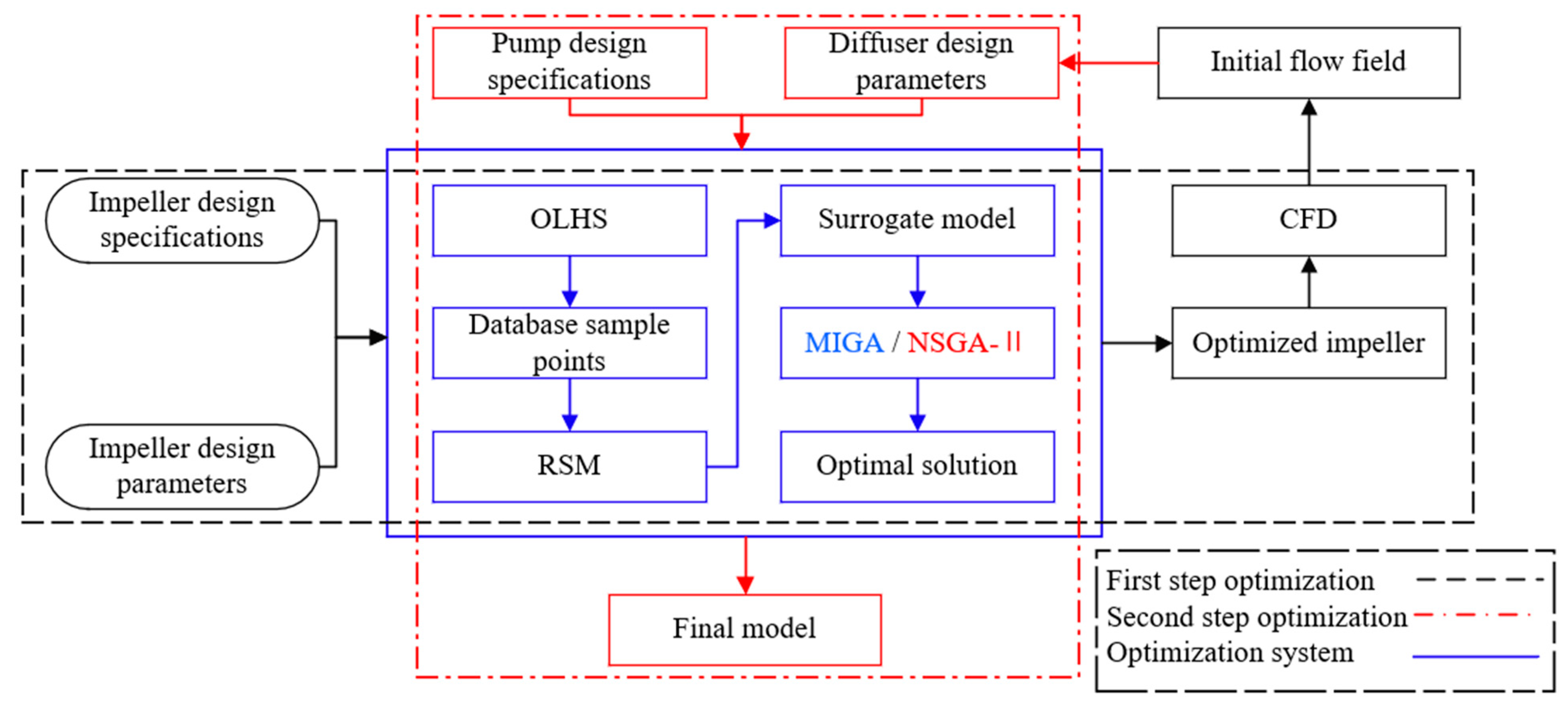
3.3. Optimization Process

The optimization process can be accelerated by constructing the approximate model between optimization objectives and design parameters. In this study, the second-order RSM was used to construct the approximate model:

$$y={\alpha }_0+{\displaystyle \sum _{i=1}^N{\alpha }_i{x}_i}+{\displaystyle \sum _{i=1}^N{\alpha }_{ii}{x}_i^2+}{\displaystyle \sum _{i\ne j}^N{\alpha }_{ij}{x}_i{x}_j}$$

(5)

Here, ${\alpha }_0$, ${\alpha }_i$, ${\alpha }_{ii}$ and ${\alpha }_{ij}$ are the undetermined coefficients and can be obtained by the least square method from the optimization objectives and design parameters.

In DOE, the optimal Latin hypercube sampling (OLHS) method was employed to generate the random, equiprobable, and orthogonally distributed sample points [28]. The structure of the sample space is consistent with the design space, which helps to reduce the number of calculation times.

A genetic algorithm (GA) was used for global optimization in the entire design space. In GA, crossover and mutation were adopted to ensure that the final result is the global optimal solution. Generally, the two main strategies for solving multi-objective optimization problems are the aggregation approach [29] and Pareto front [30]. Compared with the Pareto front, the aggregation approach has lower complexity because it converts the multi-objective optimization problem into a single-objective optimization problem through the weighted average method. However, in Pareto front, the nature of the trade-offs between optimization objectives can be more intuitively reflected.

The optimization process starts from the selection of the optimization objectives and design parameters. After determining the range of the design parameters, OLHS was used to generate different combinations of design parameters. Thereafter, IDM was used to perform 3D modeling for each parameter combination, and CFD analysis was used to calculate the model optimization objectives. Then, RSM was used to construct the approximate model between optimization objectives and design parameters. Finally, GA was used to determine the global optimal solution.

4. Redesign Setting

4.1. Design Parameters

In this study, no changes have been made to the meridional shape of the mixed flow pump; thus, the mixed flow pump can be parameterized by the parameterization of the blade. As described in Section 3.1, circulation, blade loading, and stacking have the greatest effect on blade shape in IDM. As a result, these parameters were selected as design parameters.

Generally, we assume that the circumferential distribution of the circulation is uniform. Therefore, the three-dimensional distribution of the circulation can be simplified to a two-dimensional distribution along the spanwise. Wang et al. [31,32] and Chang et al. [33] pointed out that the non-linear circulation distribution has more advantages than the linear circulation distribution in the mixed flow pump optimization design. Therefore, the curve shown in Figure 5 was used to control the circulation distribution with controlled parameters of $r{V}_{\mathrm{h}}$ and $r{V}_{\mathrm{s}}$. In this figure, $r\widetilde{V_{\theta }}=r\overline{V_{\theta }}/{\omega }^2{r}_{\mathrm{shroud}}$ is the normalized circulation, and $\tilde{r}=\left(r-r_{\mathrm{hub}}\right)/\left(r_{\mathrm{shroud}}-r_{\mathrm{hub}}\right)$ is the normalized spanwise distance.

The blade loading distribution is usually controlled by two parabolas and a connecting straight line as shown in Figure 6, where $\tilde{m}=m/m_{\mathrm{total}}$ is the normalized meridional distance. The control parameters are the loading $DRVT$ at the leading edge, the locations $NC$ and $ND$ of the connection point, and the slope $K$ of the middle straight line.

The stacking condition $\alpha$ shown in Figure 7 is usually imposed linearly along the blade trailing edge. Zangeneh [13] pointed out that it plays an important role in suppressing the flow separation in mixed flow pump. Zhu [34] also reported that it has a greater influence on the pressure pulsation in the impeller.

4.2. Optimization Setting

To determine the undetermined coefficients in Equation (5), the minimum number of sample points required is $S_{\min }=\left(N+1\right)\times \left(N+2\right)/2$, where $N$ is the number of design parameters. However, to improve the accuracy of the approximate model, the number of sample points used in this study is $2S_{\min }$. As shown in Figure 3, the impeller and diffuser of the mixed flow pump were optimized by the two-step optimization method. In

Table 2. Design parameters, constraints and optimization objectives.

	First Step of Optimization			Second Step of Optimization
	Type	Parameters	Range	Type	Parameters	Range
Design parameters	Circulation	$R{V}_{\mathrm{h}}$	0.29~0.34	Blade loading	$DRV{T}_{\mathrm{h}}$	−0.2~0.2
		$R{V}_{\mathrm{s}}$	0.29~0.34		$N{C}_{\mathrm{h}}$	0.1–0.5
	Blade loading	$DRV{T}_{\mathrm{h}}$	−0.2~0.2		$N{D}_{\mathrm{h}}$	0.5~0.9
		$N{C}_{\mathrm{h}}$	0.1~0.5		$K_{\mathrm{h}}$	−1.0~1.0
		$N{D}_{\mathrm{h}}$	0.5~0.9		$DRV{T}_{\mathrm{s}}$	−0.2~0.2
		$K_{\mathrm{h}}$	−2.0~2.0		$N{C}_{\mathrm{s}}$	0.1~0.5
		$DRV{T}_{\mathrm{s}}$	−0.2~0.2		$N{D}_{\mathrm{s}}$	0.5~0.9
		$N{C}_{\mathrm{s}}$	0.1~0.4		$K_{\mathrm{s}}$	−1.0~1.0
		$N{D}_{\mathrm{s}}$	0.4~0.9	Stacking	$\alpha$	−25.0~25.0
		$K_{\mathrm{s}}$	−2.0~2.0
	Stacking	$\alpha$	−20.0~20.0
Constraints	Impeller head at design point			Pump head at design point
Optimization objectives	Weighted efficiency of the impeller at 0.8Qdes, 1.0Qdes and 1.2Qdes			Pump efficiency at 0.8Qdes
				Pump efficiency at 1.0Qdes
				Pump efficiency at 1.2Qdes

, the design parameters (subscripts h for hub and s for shroud), constraints, and optimization objectives during the two-step optimization process were given.

In the first step of optimization, only the impeller was optimized. The design parameters are the two circulation distribution control parameters, eight blade loading distribution control parameters and stacking condition. The range of these eleven parameters is shown in Table 2. To achieve the two purposes of maximizing overall efficiency and reducing the complexity of multi-objective optimization at the same time, the aggregation approach was used in this step. The weighted efficiency of the impeller at 1.2Q_des, 1.0Q_des and 0.8Q_des was set as the optimization objective, with weights of 0.25, 0.5, and 0.25, respectively. To make the head difference between the optimized impeller and the baseline impeller fall within an acceptable range, the impeller head change at the design point of less than 3% was taken as the constraint condition. The impeller head ($H$) and efficiency ($\eta$) are calculated by Equations (6) and (7), respectively.

$$H=\frac{p_{\mathrm{out}}-p_{\mathrm{in}}}{\rho g}$$

(6)

$$\eta =\frac{(p_{\mathrm{out}}-p_{\mathrm{in}})Q}{T\omega }$$

(7)

where $p_{\mathrm{out}}$, $p_{\mathrm{in}}$, $\rho$, $g$, $\omega ,$ and $T$ are the impeller outlet total pressure, impeller inlet total pressure, fluid density, acceleration due to gravity, rotational angular velocity of the impeller, and the torque of the impeller, respectively.

After the first step of optimization, the impeller with the best performance was selected. CFD analysis was performed on the optimized impeller to extract the axial and circumferential velocity distribution at the outlet. Due to the non-uniformity of velocity distribution at the impeller outlet, directly using it as the inlet condition of the diffuser will result in the divergence of the IDM calculation, and thus the shape of the diffuser cannot be obtained. Therefore, the optimized impeller outlet velocity distribution needs to be smoothed, and the smoothed velocity will be taken as the initial condition for the second step of optimization.

In the second step of optimization, the diffuser was optimized. To reduce the hydraulic loss at the inlet of the diffuser, the circulation and flow field distribution at the diffuser inlet was set to be consistent with the optimized impeller outlet. Therefore, only the blade loading and stacking were selected as design parameters in this step. To comprehend the nature of the trade-offs made in choosing the final solution, Pareto front was used in this step, and the pump efficiencies at 1.2Q_des, 1.0Q_des, and 0.8Q_des were selected as the optimization objectives. To reduce the head change of the optimized mixed flow pump at the design point, the pump head change at the design point was restricted to less than 3%.

Therefore, in this study, to improve the accuracy of the RSM in the optimization process, the number of sample points used in the first and second steps is 156 and 110, respectively. The parameter settings for MIGA and NSGA-Ⅱ are shown in

Table 3. Parameters setting for MIGA and NSGA-Ⅱ.

MIGA		NSGA-Ⅱ
Setting	Value	Setting	Value
Population size	30	Population size	100
Number of generations	40	Number of generations	120
Number of islands	10	Crossover probability	0.9
Crossover probability	0.9	Cross distribution index	10
Mutation probability	0.05	Mutation distribution index	20
Migration probability	0.05	Initialization mode	Random

, and the number of impellers and diffusers with different configurations generated in the first and second steps are both 12,000.

4.3. Optimization Result

The iteration history of the first step optimization is shown in Figure 8, and the best impeller A is obtained after 12,000 steps of calculation. The performance predicted by RSM and CFD of optimized impeller A is shown in

Table 4. Performance comparison between computational fluid dynamics (CFD) calculation and response surface method (RSM) prediction.

	Impeller Efficiency			Pump Efficiency
	Baseline Impeller	First Step Optimization		Baseline Pump	Second Step Optimization
		RSM	CFD		RSM	CFD
${\eta }_{0.8}$	95.66		95.10	80.48	81.48	81.30
${\eta }_{1.0}$	95.05		95.84	85.21	88.55	88.89
${\eta }_{1.2}$	84.86		90.36	73.84	80.05	80.31
${\eta }_{\mathrm{w}}$	92.66	94.14	94.29
$H$	13.51	13.58	13.26	12.10	12.32	12.06

, which indicates a good consistency between the two. The weighted efficiency of the optimized impeller A is 94.29%, which is 1.63% higher than the baseline impeller. In detail, the maximum improvement of the impeller efficiency occurred at 1.2Q_des, which is 5.5%. At 1.0Q_des, the efficiency of the optimized impeller is improved by 0.79%. However, at 0.8Q_des, the efficiency of the optimized impeller is reduced by 0.56%. Moreover, the best efficiency point in the optimized impeller A is consistent with the design point, while in the baseline impeller, the best efficiency point appears at small flow conditions.

Figure 9 shows the axial and circumferential velocity distribution at the outlet of the impeller A, these values were extracted at 0.15$\tilde{r}$~0.85$\tilde{r}$ after considering the influence of the wall on the flow field. As described in Section 4.2, the velocity distribution needs to be smoothed. In this study, the widely used linear distribution assumption was used, and the results of the smoothing treatment are shown in Figure 9.

The optimization result of the second step is shown in Figure 10. In this step, the Pareto front seems separated, which means there is a trade-off relationship between the pump efficiency at 0.8Q_des (${\eta }_{0.8}$), 1.0Q_des (${\eta }_{1.0}$) and 1.2Q_des (${\eta }_{1.2}$). Figure 10a shows that ${\eta }_{0.8}$ and ${\eta }_{1.2}$ have a strong competitive relationship, while Figure 10b shows an interesting fact that ${\eta }_{1.0}$ and ${\eta }_{1.2}$ are positively correlated to some extent. After carefully considering the relationship between ${\eta }_{0.8}$, ${\eta }_{1.0}$ and ${\eta }_{1.2}$, the optimized diffuser B was selected for further study. The performance predicted by RSM and CFD of the optimized mixed flow pump is shown in Table 4. It is observed that the RSM prediction results corroborate with the CFD calculation results with the maximum error not exceeding 1%. The pump efficiency of the optimized mixed flow pump at 1.2Q_des, 1.0Q_des is 0.8Q_des is 80.31%, 88.89% and 81.30%, respectively, which is 6.47%, 3.68% and 0.82% higher than the baseline model.

Figure 11 shows the blade loading and circulation distribution of the optimized impeller and diffuser. It can be seen that the blade loading distribution at the hub and shroud of the optimized impeller A is fore-loaded and mid-loaded, respectively, while the blade loading distribution at the hub and shroud of the optimized diffuser B is fore-loaded and aft-loaded, respectively. The circulation distribution at the optimized impeller A outlet and the optimized diffuser B inlet is a second-order parabola, and the value of the circulation at the mid-span is the smallest.

5. Performance Comparison and Analysis

Figure 12 shows the performance comparison of the optimized mixed flow pump with the baseline model. When the flow rate is greater than 0.75Q_des, the pump efficiency of the optimized model is higher than the baseline model, and the location of the best efficiency point does not change. The head of the optimized model presented an interesting change compared to the baseline model. Under the design condition, the pump head of the optimized model is almost the same as the baseline model, which means that the matching optimization results meet the constraints. However, under small flow conditions, the pump head of the optimized model is lower than the baseline model, and the lower the flow rate, the greater the head difference. The decreased head and increased efficiency under small flow conditions represented the reduction of shaft power and energy-saving when the pump is operating in this area.

Table 5. Analysis of hydraulic loss.

	Baseline Model				Optimized Model
	Inlet	Impeller	Diffuser	Outlet	Inlet	Impeller	Diffuser	Outlet
0.8Qdes	0.09%	4.34%	9.72%	4.45%	0.09%	4.90%	9.18%	3.62%
0.9Qdes	0.13%	4.16%	7.56%	4.01%	0.13%	3.78%	6.33%	2.73%
1.0Qdes	0.18%	4.95%	5.32%	3.40%	0.18%	4.16%	3.85%	2.03%
1.1Qdes	0.25%	8.14%	3.52%	2.99%	0.25%	5.65%	3.33%	2.16%
1.2Qdes	0.37%	15.14%	5.13%	3.92%	0.36%	9.64%	5.04%	3.08%

shows the comparison of hydraulic losses of each flow passage component between the optimized model and baseline model under different flow rates. Compared with the baseline model, the hydraulic loss of the optimized impeller under large flow conditions is effectively suppressed, and the hydraulic loss of the optimized diffuser under the design condition is significantly reduced. Moreover, the hydraulic loss of the inlet pipe is positively related to the flow rate and independent of the impeller. However, the hydraulic loss of the outlet pipe is related to both the diffuser and flow rate. Compared with the baseline model, the hydraulic loss of the optimized model outlet pipe is reduced under all flow conditions.

To clarify the reasons for the change of hydraulic loss in detail, the internal flow field of the optimized model and the baseline model were analyzed and compared. The streamline contours and total pressure on the mid-span of the baseline model and optimized model are shown in Figure 13. At 0.8Q_des and 1.0Q_des, a large-scale flow separation occurs at the diffuser outlet of the baseline model, which not only increased the hydraulic losses at the diffuser but also at the outlet pipe. At 1.2Q_des, an obvious low-pressure region appeared on the working surface near the impeller inlet of the baseline model. Zhang [35] pointed out that this region has a great influence on the blade vibrations and pressure fluctuation. After the matching optimization, the flow separation in the optimized diffuser was effectively suppressed, especially at 1.0Q_des, and the low-pressure region at the impeller inlet at 1.2Q_des was also weakened. As Zangeneh [12,13,36] mentioned, in the optimization design of mixed flow pump, the flow separation can be effectively suppressed by fore-loading at the hub and aft-loading at the shroud. This paper verifies this point of view again.

The comparison of the total pressure distribution along the streamline between the baseline model and the optimized model is shown in Figure 14. The horizontal axis is the standardized streamline distance $\tilde{S}$, $\tilde{S}=0$ means at the impeller inlet and $\tilde{S}=2$ means at the diffuser outlet. It can be seen that the total pressure rises rapidly between 0.2$\tilde{S}$~0.8$\tilde{S}$ due to the work done by the impeller to the fluid. However, the total pressure drops rapidly between 0.8$\tilde{S}$~1.2$\tilde{S}$, because the fluid in this interval has just left the blade zone of the impeller and has not yet entered the blade zone of the diffuser. Compared with the baseline model, the hydraulic loss of the optimized model in this interval was significantly reduced, which may be related to the setting of the diffuser inlet conditions during the matching optimization. The total pressure decreases slowly between 1.2$\tilde{S}$~2$\tilde{S}$ due to the rectification effect of the diffuser.

6. Conclusions

To further improve the optimization effect of the mixed flow pump, a matching optimization strategy of impeller and diffuser was proposed in this study. The matching optimization process was divided into two steps. In the first step of optimization, only the impeller was optimized. In the second step of optimization, the diffuser was optimized. Some important conclusions are as follows:

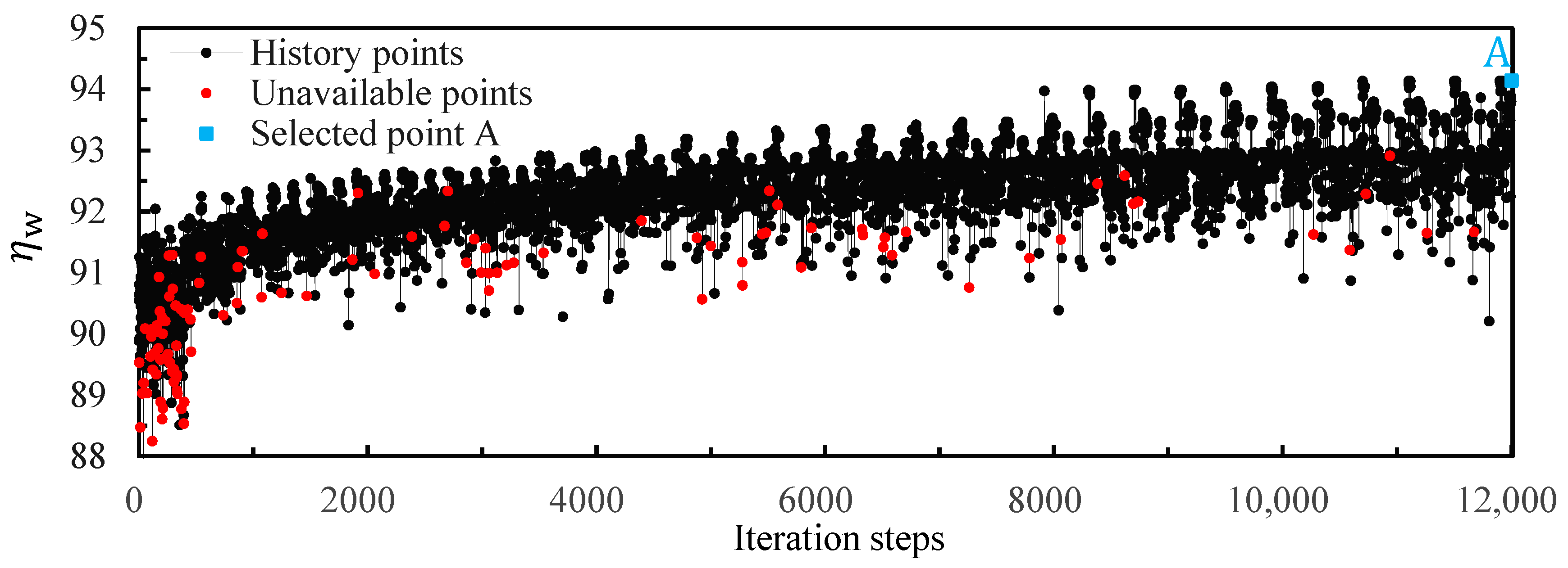
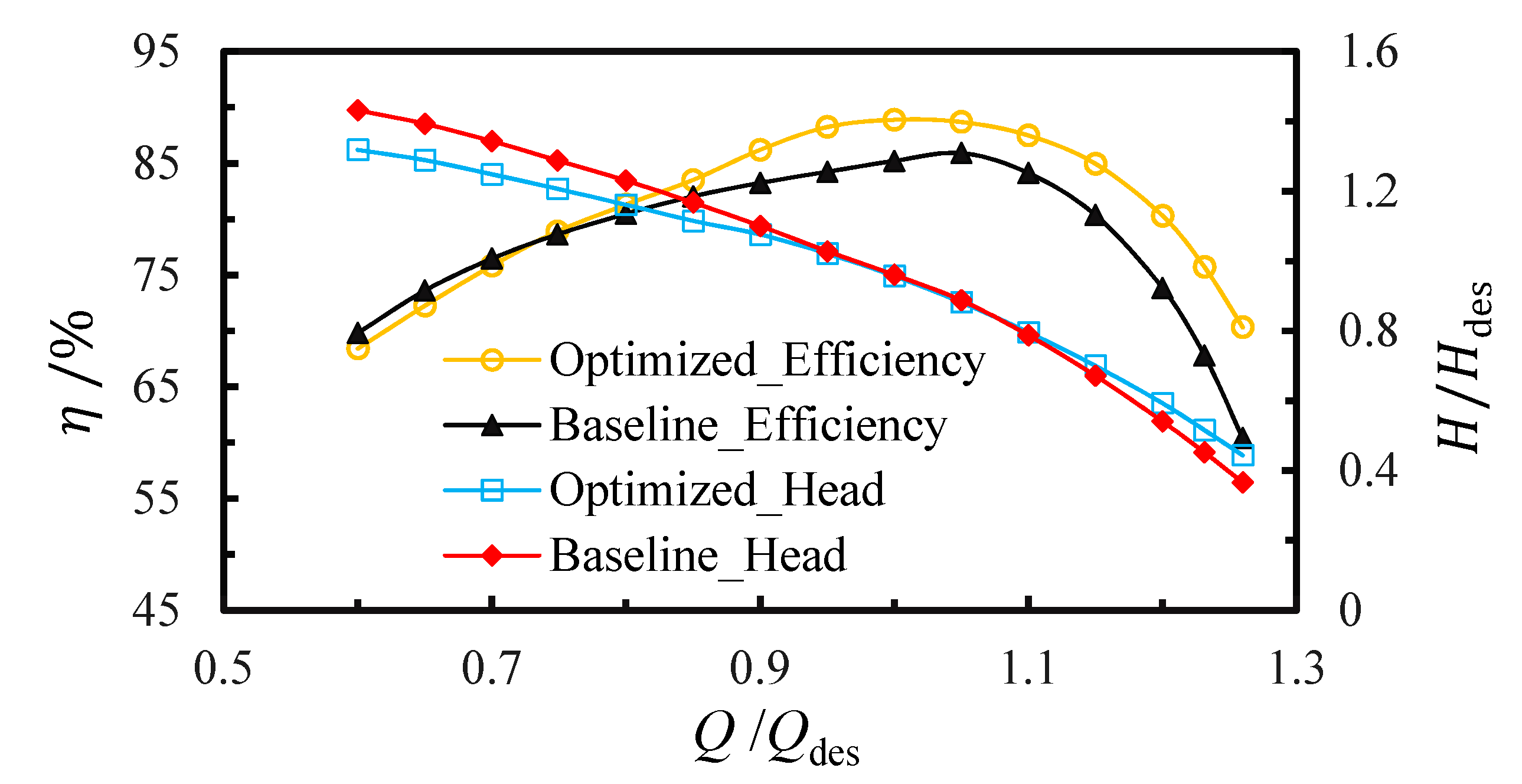
• After the first step of optimization, the weighted efficiency of the optimized impeller A is 1.63% higher than the baseline impeller. In detail, the impeller efficiency of the optimized impeller A at 1.2Q_des and 1.0Q_des is 5.5% and 0.79% higher than the baseline impeller, respectively, but 0.56% lower at 0.8Q_des. Besides, the best efficiency point in the optimized impeller A is consistent with the design point, while in the baseline impeller, the best efficiency point appears at small flow conditions.
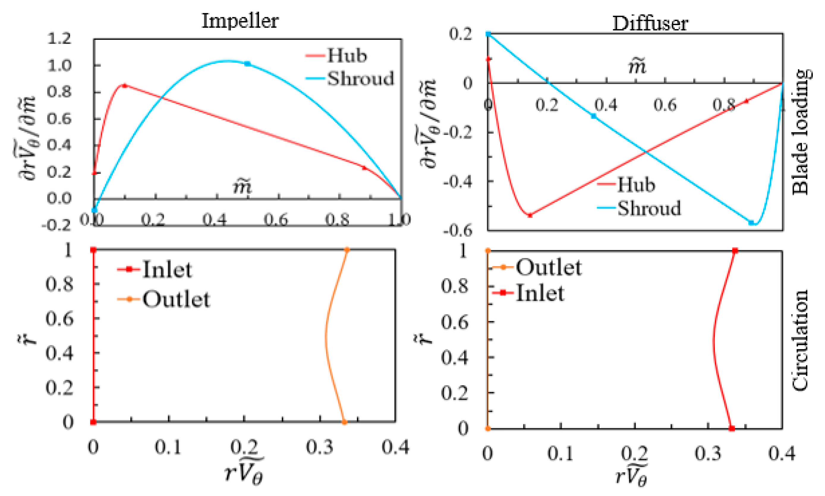
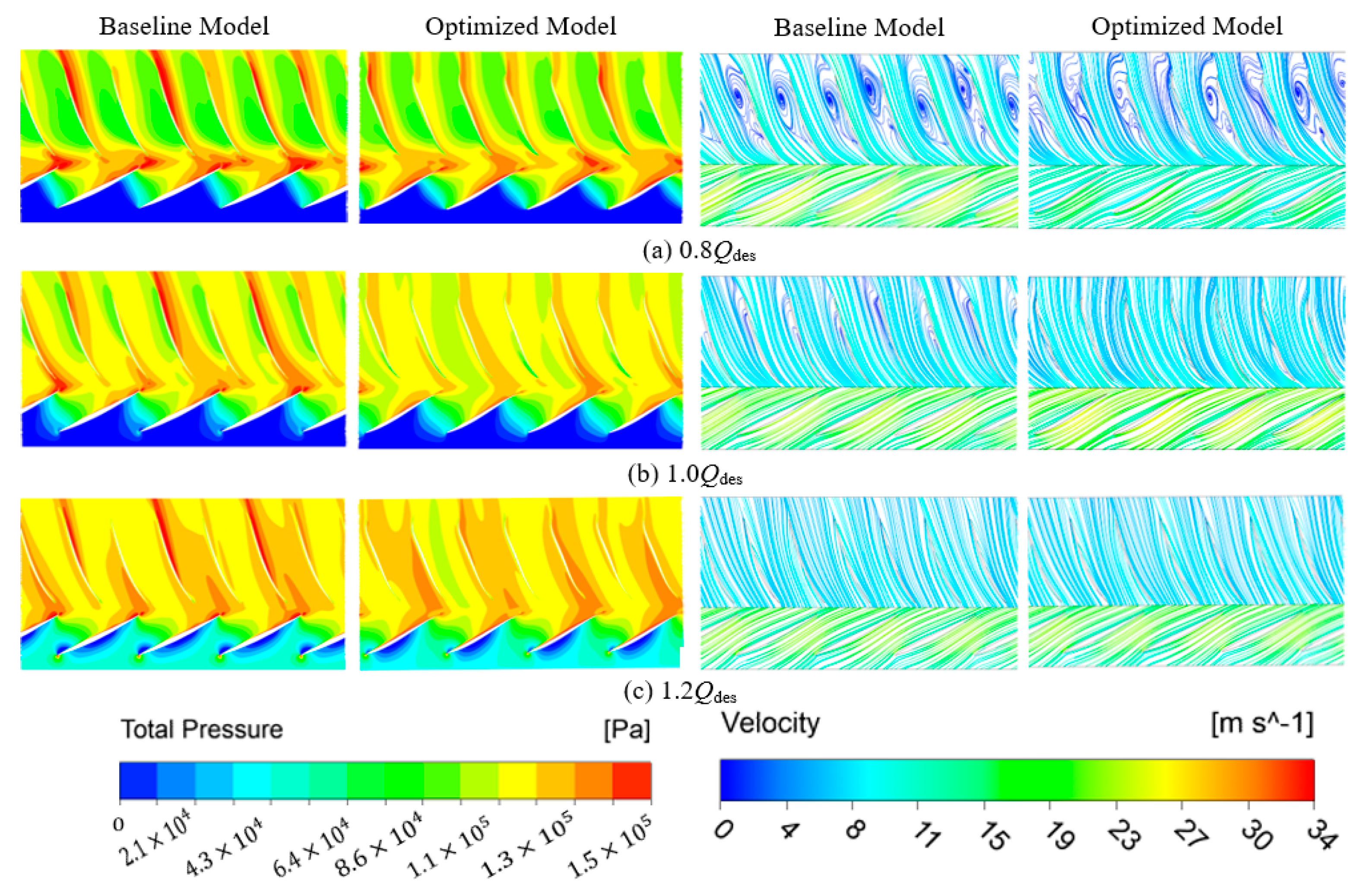
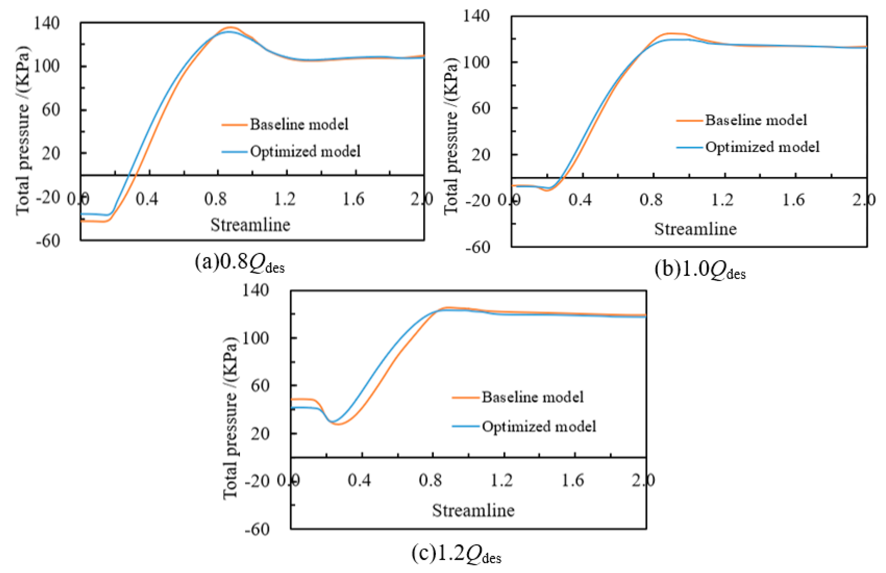
• In the matching optimization, the circulation and flow field distribution at the diffuser inlet in IDM was set to be consistent with the optimized impeller outlet, which helps to reduce the hydraulic loss at the diffuser inlet. Compared with the baseline diffuser, the hydraulic loss of the optimized diffuser B at 1.2Q_des, 1.0Q_des, and 0.8Q_des reduced by 0.09%, 1.47%, and 0.54%, respectively.
• The diffuser has a great impact on the hydraulic loss of downstream components. The hydraulic loss of the optimized model outlet pipe at 1.2Q_des, 1.0Q_des, and 0.8Q_des is 0.84%, 1.37%, and 0.83% lower than the baseline diffuser outlet pipe, respectively.
• In total, the pump efficiency of the optimized model at 1.2Q_des, 1.0Q_des, and 0.8Q_des is 80.31%, 88.89% and 81.30%, respectively. These efficiencies correspond to 6.47%, 3.68%, and 0.82% improvement over the baseline model.

In summary, the matching optimization strategy proposed in this study is effective and can overcome the shortcomings of single-component optimization and thereby further improve the overall hydraulic performance of the mixed flow pump. The results of this study can also provide guidance for the optimization of other rotating machinery.

References

1. Wu, J.; Shimmei, K.; Tani, K.; Niikura, K.; Sato, J. CFD-Based Design Optimization for Hydro Turbines. J. Fluids Eng. 2007, 129, 159–168. [Google Scholar] [CrossRef]
2. Ma, Z.; Zhu, B.S.; Rao, C.; Shangguan, Y.H. Comprehensive Hydraulic Improvement and Parametric Analysis of a Francis Turbine Runner. Energies 2019, 12, 307. [Google Scholar] [CrossRef] [Green Version]
3. Chikh, M.A.A.; Belaidi, I.; Khelladi, S.; Hamrani, A.; Bakir, F. Coupling of Inverse Method and Cuckoo Search Algorithm for Multiobjective Optimization Design of an Axial Flow Pump. Proc. Inst. Mech. Eng. Part A J. Power Energy 2019, 233, 988–1006. [Google Scholar] [CrossRef]
4. Meng, F.; Li, Y.; Yuan, S.; Wang, W.; Zheng, Y.; Osman, M.K. Multiobjective Combination Optimization of an Impeller and Diffuser in a Reversible Axial-Flow Pump Based on a Two-Layer Artificial Neural Network. Processes 2020, 8, 309. [Google Scholar] [CrossRef] [Green Version]
5. Shi, L.; Zhu, J.; Tang, F.; Wang, C. Multi-Disciplinary Optimization Design of Axial-Flow Pump Impellers Based on the Approximation Model. Energies 2020, 13, 779. [Google Scholar] [CrossRef] [Green Version]
6. Pei, J.; Gan, X.; Wang, W.; Yuan, S.; Tang, Y. Multi-objective Shape Optimization on the Inlet Pipe of a Vertical Inline Pump. J. Fluids Eng. 2019, 141, 061108. [Google Scholar] [CrossRef]
7. Wang, W.J.; Yuan, S.Q.; Pei, J.; Zhang, J.F. Optimization of the Diffuser in a Centrifugal Pump by Combining Response Surface Method with Multi-island Genetic Algorithm. Proc. Inst. Mech. Eng. Part E J. Process. Mech. Eng. 2017, 231, 191–201. [Google Scholar] [CrossRef]
8. Shim, H.S.; Afzal, A.; Kim, K.Y.; Jeong, H.S. Three-objective Optimization of a Centrifugal Pump with Double Volute to Minimize Radial Thrust at Off-design Conditions. Proc. Inst. Mech. Eng. Part A J. Power Energy 2016, 230, 598–615. [Google Scholar] [CrossRef]
9. Kim, S.; Jeong, U.-B.; Lee, K.-Y.; Kim, J.-H.; Yoon, J.-Y.; Choi, Y.-S. Multi-objective Optimization for Mixed-flow Pump with Blade Angle of Impeller Exit and Diffuser Inlet. J. Mech. Sci. Technol. 2017, 31, 5099–5106. [Google Scholar]
10. Suh, J.-W.; Yang, H.-M.; Kim, Y.-I.; Lee, K.-Y.; Kim, J.-H.; Joo, W.-G.; Choi, Y.-S. Multi-objective Optimization of a High Efficiency and Suction Performance for Mixed-flow Pump Impeller. Eng. Appl. Comput. Fluid Mech. 2019, 13, 744–762. [Google Scholar] [CrossRef] [Green Version]
11. Zangeneh, M. A Compressible 3D Design Method for Radial and Mixed Flow Turbomachinery Blades. Int. J. Numer. Methods Fluids 1991, 13, 599–624. [Google Scholar] [CrossRef]
12. Goto, A.; Takemura, T.; Zangeneh, M. Suppression of Secondary Flows in a Mixed-Flow Pump Impeller by Application of Three-Dimensional Inverse Design Method: Part 2—Experimental Validation. J. Turbomach. 1996, 118, 544–551. [Google Scholar] [CrossRef]
13. Zangeneh, M.; Goto, A.; Takemura, T. Suppression of Secondary Flows in a Mixed-Flow Pump Impeller by Application of Three-Dimensional Inverse Design Method: Part 1—Design and Numerical Validation. J. Turbomach. 1996, 118, 536–543. [Google Scholar] [CrossRef]
14. Huang, R.F.; Luo, X.W.; Ji, B.; Wang, P.; Yu, A.; Zhai, Z.H.; Zhou, J.J. Multi-objective Optimization of a Mixed-Flow Pump Impeller Using Modified NSGA-II Algorithm. Sci. China Technol. Sci. 2015, 58, 2111–2130. [Google Scholar] [CrossRef]
15. Yiu, K.F.C.; Zangeneh, M. Three-Dimensional Automatic Optimization Method for Turbomachinery Blade Design. J. Propuls. Power 2000, 16, 1174–1181. [Google Scholar] [CrossRef]
16. Zhu, Y.J.; Ju, Y.P.; Zhang, C.H. An Experience-independent Inverse Design Optimization Method of Compressor Cascade Airfoil. J. Power Energy 2018, 233, 431–442. [Google Scholar] [CrossRef]
17. Zhu, B.; Wang, X.; Tan, L.; Zhou, D.; Zhao, Y.; Cao, S. Optimization Design of a Reversible Pump–Turbine Runner with High Efficiency and Stability. Renew. Energy 2015, 81, 366–376. [Google Scholar] [CrossRef]
18. Yang, W.; Xiao, R.F. Multiobjective Optimization Design of a Pump–turbine Impeller Based on an Inverse Design using a Combination Optimization Strategy. J. Fluid. Eng. 2014, 136, 249–256. [Google Scholar] [CrossRef]
19. Zangeneh, M.; Daneshkhah, K. A Fast 3D Inverse Design Based Multi-Objective Optimization Strategy for Design of Pumps. In Proceedings of the ASME 2009 Fluids Engineering Division Summer Meeting, Vail, CO, USA, 2–6 August 2009. [Google Scholar]
20. Wang, P.; Vera-Morales, M.; Vollmer, M.; Zangeneh, M.; Zhu, B.S.; Ma, Z. Optimization of a Pump-as-turbine Runner Using a 3D Inverse Design Methodology. In Proceedings of the 29th IAHR Symposium on Hydraulic Machinery and Systems, Kyoto, Japan, 16–21 September 2018; Volume 240. [Google Scholar]
21. Bonaiuti, D.; Zangeneh, M. On the Coupling of Inverse Design and Optimization Techniques for the Multiobjective, Multipoint Design of Turbomachinery Blades. J. Turbomach. 2009, 131, 134–149. [Google Scholar]
22. Bonaiuti, D.; Zangeneh, M.; Aartojarvi, R.; Eriksson, J. Parametrical Design of a Waterjet Pump by Means of Inverse Design, CFD Calculations and Experimental Analyses. J. Fluid. Eng. 2010, 132, 201–215. [Google Scholar] [CrossRef]
23. Yang, W.; Lei, X.; Zhang, Z.; Li, H.; Wang, F. Hydraulic Design of Submersible Axial-flow Pump Based on Blade Loading Distributions. Trans. Chin. Soc. Agric. Mach. 2017, 48, 179–187. (In Chinese) [Google Scholar]
24. Yin, J.; Wang, D. Review on Applications of 3D Inverse Design Method for Pump. Chin. J. Mech. Eng. 2014, 27, 520–527. [Google Scholar] [CrossRef]
25. Hawthorne, W.R.; Wang, C.; Tan, C.S.; McCune, J.E. Theory of blade design for large deflections: Part I-Two dimensional cascades. Trans. ASME J. Eng. Gas Turb. Power 1984, 106, 346353. [Google Scholar] [CrossRef]
26. Hellsten, A.; Laine, S. Extension of the k-omega-SST Turbulence Model for Flows over Rough Surfaces. In Proceedings of the 22nd Atmospheric Flight Mechanics Conference, New Orleans, LA, USA, 11–13 August 1997. [Google Scholar]
27. Menter, F.R.; Galpin, P.F.; Esch, T.; Kuntz, M.; Berner, C. CFD Simulations of Aerodynamic Flows with a Pressure-based Method. In Proceedings of the 24th International congress of the aeronautical sciences, Yokohama, Japan, 29 August–3 September 2004. [Google Scholar]
28. Pebesma, E.J.; Heuvelink, G.B. Latin Hypercube Sampling of Gaussian Random Fields. Technometrics 1999, 41, 303–312. [Google Scholar] [CrossRef]
29. Coello, C.A.C. A Comprehensive Survey of Evolutionary-Based Multiobjective Optimization Techniques. Knowl. Inf. Syst. 1999, 1, 269–308. [Google Scholar] [CrossRef]
30. Srinivas, N.; Deb, K. Multiobjective Optimization Using Nondominated Sorting in Genetic Algorithms. Evolut. Comput. 1994, 2, 221–248. [Google Scholar] [CrossRef]
31. Wang, M.C.; Li, Y.J.; Yuan, J.P.; Meng, F.; Appiah, D.; Chen, J.Q. Comprehensive Improvement of Mixed-flow Pump Impeller Based on Multi-objective Optimization. Processes 2020, 8, 905. [Google Scholar] [CrossRef]
32. Wang, M.C.; Li, Y.J.; Yuan, J.P.; Chen, J.Q.; Zheng, Y.H.; Yang, P.H. Performance of Mixed Flow Pump under Condition of Non-linear Distribution of Impeller Exit Circulation. Chin. Soc. Agric. Mach. 2020, 51, 204–211. (In Chinese) [Google Scholar]
33. Chang, S.P.; Shi, Y.F.; Zhou, C.; Ding, J. Effect of Exit Circulation Distribution on Performances of Mixed-flow Pump. Trans. Chin. Soc. Agric. Mach. 2014, 45, 89–93. (In Chinese) [Google Scholar]
34. Zhu, B.S.; Tan, L.; Wang, X.H.; Ma, Z. Investigation on Flow Characteristics of Pump-Turbine Runners with Large Blade Lean. J. Fluids Eng. 2017, 140. [Google Scholar] [CrossRef]
35. Zhang, P.Y.; Zhu, B.S.; Zhang, L.F. Numerical Investigation on Pressure Fluctuations Induced by Interblade Vortices in a Runner of Francis Turbine. Large Electron. Mach. Hydraul. Turbine 2009, 35, 35–38. (In Chinese) [Google Scholar]
36. Zangeneh, M.; Goto, A.; Harada, H. On the Design Criteria for Suppression of Secondary Flows in Centrifugal and Mixed Flow Impellers. J. Turbomach. 1998, 120, 723. [Google Scholar] [CrossRef]
Figure 1. Baseline model.
Processes 09 00260 g001
Figure 2. Performance curves for the baseline model.
Processes 09 00260 g002
Figure 3. Flowchart of optimization strategy.
Processes 09 00260 g003
Figure 4. Mesh of computational domains.
Processes 09 00260 g004
Figure 5. Circulation distribution at the impeller outlet and diffuser inlet.
Processes 09 00260 g005
Figure 6. Blade loading distribution along the streamline.
Processes 09 00260 g006
Figure 7. Stacking condition.
Processes 09 00260 g007
Figure 8. Optimization results of the first step.
Processes 09 00260 g008
Figure 9. Velocity distribution at the impeller outlet and diffuser inlet.
Processes 09 00260 g009
Figure 10. Optimization results of second step. (a) η 0.8 vs. η 1.2 ; (b) η 1.0 vs. η 1.2 .
Processes 09 00260 g010
Figure 11. Blade loading distribution and circulation distribution of optimized impeller and diffuser.
Processes 09 00260 g011
Figure 12. Performance comparison between optimized model and baseline model.
Processes 09 00260 g012
Figure 13. Comparison of the internal flow field between the optimized model and baseline model.
Processes 09 00260 g013
Figure 14. Total pressure distribution along the streamline.
Processes 09 00260 g014