Abstract
Microwave drying of suspensions of lignocellulosic fibers has the potential to produce porous foam materials that can replace materials such as expanded polystyrene, but the design and control of this drying method are not well understood. The main objective of this study was to develop a microwave drying model capable of predicting moisture loss regardless of the shape and microwave power input. A microwave heating model was developed by coupling electromagnetic and heat transfer physics using a commercial finite element code. The modeling results predicted heating time behavior consistent with experimental results as influenced by electromagnetic fields, waveguide size and microwave power absorption. The microwave heating modeling accurately predicted average temperature increase for water domain at 360 and 840 W microwave power inputs. By dividing the energy absorption by the heat of vaporization, the amount of water evaporation in a specific time increment was predicted leading to a novel method to predict drying. Using this method, the best time increments, and other parameters were determined to predict drying. This novel method predicts the time to dry cellulose foams for a range of sample shapes, parameters, material parameters. The model was in agreement with the experimental results.
1. Introduction
Porous foam structures have been extensively used for a wide range of industrial applications including thermal insulation [1], packaging applications [2], energy storage [3] and biomedical applications [4]. Over the last few decades, petroleum-based plastics such as polyurethane, polyethylene and polystyrene became the most widely used foam materials attributed to their attractive features [5]. However, non-biodegradability of plastics poses a serious threat to the environment by creating ocean plastic pollution and landfill issues with materials that can take hundreds of years to break down into soil or incineration concerns causing severe air pollution and imparting high cost [6]. Sustainable porous cellulose nanofibrils (CNF) foams are being considered as a novel renewable product since they are environmentally friendly, sustainable, and bestow significantly improved properties over plastics [7]. CNF is a major group of cellulose nanomaterials that is mainly produced from softwood bleached pulp through a mechanical fibrillation process [8]. The binder applications of CNFs have recently attracted a lot of attention and various products such as paper laminates [9], particleboard [10], fiberboard [11] and wallboard [12] that take advantage of the impressive binder properties of CNF have been developed. These binder properties can be exploited to generate rigid foams if a method to produce them can be found.
Many groups have reported on the fabrication technique of these foams based on freeze-drying [13,14,15]. During freeze-drying, ice crystals are removed by sublimation process at low pressure to give a porous structure; the final porosity depends on the initial solids level and can be adjusted over a wide range. However, the rate of heat and mass transfer process in freeze-drying is low leading to high capital costs to produce material in this manner. Microwave drying, an alternative to freeze-drying, a rapid dehydration process has been found to be successfully applied to generate porous materials [16]. Microwaves, a form of electromagnetic radiation lies in the frequency range of 0.3–300 GHz [17], lending themselves in many interesting applications including heating, drying, sintering, vulcanizing and others. During microwave processing, volumetric heating takes place due to the penetration of microwaves into the materials. Such an approach can be dominated by material size, microwave power and dielectric properties of the material etc. that complicates the energy absorption behavior. Several researchers have studied microwave heating for a wide range of materials such as coal [17], food [18], minerals [19], and wood [20]. Pitchai et al. [18] successfully developed a microwave heating finite element (FE) model for chicken nuggets and mashed potatoes to identify cold spot locations. Rattachendo [20] developed a three-dimensional model based on a finite difference method for microwave heating of wood revealing that electromagnetic fields and temperature distributions were influenced by the sample size, frequency and irradiation time. While the modeling of heating with microwave can be simply regarded as a coupling of electromagnetic radiation and heat transfer, drying of materials is complex because of the phase change of the moisture, transport of moisture from the sample, and the potential change of the sample size and properties with moisture loss. Microwaves penetrate the sample and generate volumetric heating; this heating can generate pressure gradients inside the sample due to the formation of vapors.
Finite element (FE) methods numerically solve differential equations widely used in different fields because of the decomposition ability of a complex three-dimensional geometry into a number of elements of simple geometry, typically, tetrahedral and hexahedral in shape [21,22]. FE models for microwave heating consider Maxwell’s equation or Lambert’s law for power absorption. Lambert’s law is more appropriate for semi-infinite samples and determines the electric field bypassing the power distribution term. Most studies and models of microwave drying involve coupling physics such as electromagnetics, heat and mass transfer [23,24,25]. Feng et al. [23] employed a finite difference technique to develop heat and mass transfer model of diced apples under microwave. Gulati et al. [24] proposed a model that includes electromagnetic heating, multiphase transport and deformation of material and can be used for drying of hygroscopic porous materials. A coupled electromagnetic and heat transfer model to examine the effect of microwave heating on coal was reported by Huang et al. [25]. Salagnac et al. [26] developed a one-dimensional numerical model under infrared and microwave drying methods. Energy input in the model determined by the Lambert-Beer law and hygrothermal behavior of porous material was described by the energy conservations law. He et al. [27] reported a novel micro combustor with internal spiral fins to investigate thermal performance and exergy efficiency for a microphotovoltaic system. The results showed that micro combustor with eight fins exhibits the highest exergy efficiency. A comprehensive 3D-FE model with Lambert’s law for microwave power absorption was developed by Kadem et al. [28] to simulate free liquid, vapor and bound water movement during microwave drying of wood. Khan et al. [29] studied an intermittent convective microwave drying (IMCD) process with a computational fluid dynamics (CFD) model to accelerate evaporation. As the heat and mass transfer varied spatially throughout the sample, the IMCD model significantly affected drying kinetics.
Comparatively, a limited amount of microwave modeling has been performed on lignocellulose foams. Prior microwave drying efforts of lignocellulose foam materials have mostly been studied experimentally. In this work, a robust microwave modeling is proposed to examine drying behavior of lignocellulose foam materials and the effect of different parameters on drying. Here, a three-dimensional FE model that couples electromagnetic and heat transfer physics is proposed to predict heating and drying of foam materials based on lignocellulosic fibers and CNF. The heating and drying model considers two physics: electromagnetic fields based on the Maxwell’s equation and heat transfer determined from the energy equation. Heating predictions are compared to experimental results for water for several scenarios. The drying rate of samples was predicted with a novel iterative procedure that calculates the energy absorption by the sample, converts this energy to the amount of water evaporated using the heat of vaporization, and adjusts the water content of the domain to account for evaporation. Various sample geometries are modeled, and the model predictions are compared to experimental results.
2. Materials and Methods
2.1. Model Formulation
The coupled electromagnetic and heat transfer model for microwave heating and drying of foams was developed using finite element modeling in COMSOL Multiphysics 5.5a [30]. The simulations were carried out on a computer with Intel Core i7-6700, 3.40 GHz processor, 16 GB RAM memory and 64-bit Windows 10 operating system. An accurate heating and drying modeling requires a correct geometry model of the microwave oven cavity with waveguide for the solution of electromagnetic analysis.
The geometry model for experimental heating and drying was developed based on a microwave oven (Model number: LMC1575; LG Corporation, Seoul, Korea) of rated power equipped with a Smart Inverter that provides the opportunity to customize the power input. The geometry model includes the oven cavity, waveguide, and glass plate. The dimensions of the geometry model match the actual dimensions of the microwave used in the experiment. According to the dimensions of the microwave provided in the oven manual the geometry model was developed. Figure 1a shows the schematic of the microwave oven system used for modeling. The microwave is connected to a microwave source via a rectangular waveguide operating in the transverse electric (TE10) mode of excitation. In the TE10 mode, the electric field is perpendicular to the direction of propagation through a waveguide. The oven cavity is filled with air. The waveguide was located at the center of the left side wall. Walls of the microwave oven and waveguide are made of copper. A glass plate was placed at the center of the microwave. In this study, heating and drying were considered for different components. Microwave irradiation of water required a glass beaker placed at the center of the glass plate. The features of the microwave geometry model with dimensions and materials are listed in Table 1.
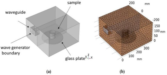
Figure 1.
Schematic of the microwave oven system (a) and meshed geometry (b).

Table 1.
Features of microwave oven system with dimensions and materials.
In this study, multiple components of different shapes and physical properties, e.g., foam and water are employed to validate the model. Lignocellulose foam preparation requires the combination of CNF, wood fiber and water, which is then dried to create a porous medium composed of CNF and wood fiber. The following assumptions were made to simulate microwave heating and drying analysis of porous materials and water.
- Microwave cavity walls and waveguides are made of copper which works as a perfect conductor and reflects microwave. Dielectric loss and thickness of the walls are negligible.
- Microwave frequency of has no electric field components or fluctuation in the direction of propagation.
- The time-dependent coupled electromagnetic and heat transfer analysis influences the temperature and dielectric properties of the sample. Electromagnetic analysis considers the wave equations under frequency domain to determine the electric field for a defined time. Heat transfer in porous media nodes were used to analyze temperature increment for heating and drying simulations. The calculated temperature and updated dielectric properties at the end of each time increment were used as input for the following time-increment.
- CNF and thermal mechanical pulp (TMP) fiber are considered as a single entity. Microwave drying of cellulose foam materials only considers water occupying the entire domain to avoid the complexity of heat transfer in the fibrous network, which is further explained in Section 2.5. Therefore, the volume fraction of the solid domain in the porous media node was zero.
- The physical properties of the materials such as permittivity, permeability, temperature, density, thermal conductivity, and specific heat capacity are isotropic and constant. The initial temperature of the materials is homogeneous.
- All materials exhibit non-magnetic behavior.
2.2. Governing Equations
The evaluation of electromagnetic heat generation of any material can be conducted by applying Maxwell’s equation. Molecular vibration generates the oscillating electric field through which microwave electromagnetic radiation is converted to thermal energy. Maxwell’s equation offers a rigorous formulation which governs the electromagnetic field distribution in space and time. This approach is accurate for various geometries ranging from spherical, cylindrical, and rectangular to hollow shapes. Electromagnetic waves lose their energy while travelling through a lossy dielectric medium. The electromagnetic field distribution was calculated by frequency domain Maxwell’s equation:
where, denotes the relative permeability, E is the electric field intensity, is the free space wave number, is the relative permittivity, is the conductivity, is the angular frequency and is the permittivity of the vacuum. The free space wave number () can be defined as [31]
where is the speed of light in vacuum (). The relative permittivity can be expressed as [32]
where is the dielectric constant which describes the ability of materials to store electromagnetic energy and is the dielectric loss factor which indicates the dissipation ability of electrical energy to heat energy.
Electromagnetic waves interact with dielectric materials and part of the electromagnetic energy is converted to thermal energy. The generated thermal energy, (), is directly proportional to the square of the electric field strength and dielectric loss factor [33]:
Once the electric field strength is known from Equation (1), the thermal energy can be calculated from Equation (4). Heat transfer during microwave irradiation can be modelled using Fourier’s law:
where, is the density of the material (), is the specific heat capacity , is the effective heat conductivity and T is the temperature (K).
2.3. Boundary Conditions
The impedance boundary condition is applied at the walls of the cavity and the waveguides where the field is known to penetrate only a short distance outside the boundary:
where, and are the relative permittivity, relative permeability, and electrical conductivity of the material, respectively and is the source electric field ().
The port boundary condition can launch and absorb specific modes, and thereby, excite the model. It is applied at the entrance of waveguide to specify wave types. In this study, electromagnetic waves are assumed to propagate through a rectangular waveguide with TE10 mode. The cutoff frequency for different modes is given by [17]:
where m and n are the mode numbers (for TE10 mode, m = 1, n = 0), a and b are the dimensions of the cross-section of rectangular waveguide, and c denotes the speed of light. The port boundary requires a propagation constant, which is given by the following expression [17]:
The perfect electric conductor boundary condition is applied on the microwave cavity and waveguide walls that considers the tangential component of the electric field is zero:
For heat transfer analysis, thermal insulation boundary condition is employed to define no heat flux across the boundaries of microwave cavity and waveguide walls:
2.4. Meshing and Simulation Techniques
The microwave geometry model was established by combining different features of different materials. The accuracy of the FE model considerably depends on the meshing scheme, i.e., element size and shape. The commercial code offers two meshing sequence types: physics-controlled mesh and user-controlled mesh. In this study, physics-controlled mesh was enabled, creating a mesh for all features automatically. Discretization of the model was generated using the default tetrahedral element. In this study, multiple samples were considered for microwave irradiation. Variation of the element sizes were observed due to mesh refinement for different domains (cylindrical sample- size: 0.08–2.28 mm, elements: 81,188; glass beaker and plate- size: 0.46–15.3 mm, elements: 18,910; cavity domain- size: 0.46–15.3 mm, elements: 79,143). The total number of elements in the entire geometry was 179,241 with averaged element quality of 0.74 as shown in Figure 1b. Liu et al. [34] stated a relation between free space wavelength () and finite element mesh size of dielectric material at 2.45 GHz to obtain reliable results and faster computational time:
were, h is the element size, is the free space wavelength and is the dielectric constant of water. Equation (11) signifies the best mesh size for the water sample should be 2.3 mm. Element size for water sample using the physics-controlled meshing is accurate enough to obtain reliable results. Huang et al. [25] also employed physics-controlled meshing for the microwave heating modeling on coal.
Microwave heating of water was analyzed using the FE model. Analyses on liquid are more challenging as they consist of fluid motion causing the interactions of electromagnetic fields, microwave field, and temperature distributions. In view of these complexities, modeling on heating of water was performed considering a solid domain or not accounting for any fluid motion. A glass beaker was considered to hold the water sample. This model provides a baseline to compare with the actual behavior. Modeling of microwave heating was performed considering a stationary glass plate. Electromagnetic field distribution for a defined time-increment under frequency domain was calculated by Maxwell’s Equation (1). The dissipated power density inside the water sample was calculated using Equation (4). An iterative solver technique named generalized minimal residual (GMRES) method was used to solve the electromagnetic analysis. Microwave power is considered as a heat source for the energy conservation equation. Time-dependent heat transfer analysis was solved using Equation (5) with a parallel sparse direct solver (PARDISO). The initial temperature of the water sample was . Time required to attain average temperature of the sample signifies the heating time. Depending on the heating time, the modeling was continued and produced a temperature distribution for the water sample. Table 2 lists the input parameters for the microwave heating modeling of water.
Table 2.
Input parameters for microwave heating of water.
2.5. Mass Transfer Modeling
Microwave drying modeling of foam materials poses a challenge as it involves simultaneous heat and mass transfer where water migrates from the materials to the microwave cavity and into the room through evaporation. As described above, previously proposed models are complex with a number of parameters and assumptions. In addition, water movement to the sample boundaries may be a combination of capillary flow, vapor-driven flow, or diffusion. A simple and novel approach is proposed here that uses an iterative procedure to reduce the complexity of the situation. The same coupled electromagnetic and heat transfer analysis explained in the previous section for microwave heating are utilized to predict the temperature distribution of the domain assuming that the water does not evaporate. The initial temperature of the solid domain was assumed to be 100 °C and the temperature was allowed to increase to values well above the boiling point of water. In reality, once water is over its boiling point, it is a vapor and will leave the structure through some mechanism. The temperature gradient of the solid domain originating from microwave irradiation for a time-increment was averaged to quantify the temperature change. The energy absorbed was calculated based on the mass of the material, specific heat and temperature change due to heating. This energy was assumed to provide the heat of vaporization of water. Therefore, the mass of water evaporated M in a given time increment is given as:
where, m is the mass of water in the sample, is specific heat of water and DT is change of temperature predicted. The heat of vaporization of water is . Therefore, for a set increment in time, the average temperature change of the sample is used to calculate the heat absorbed by the sample. It is important to note that both free and bound water are assumed to have the same heat of vaporization. Therefore, there is no difference in the drying model for the system. However, it is understood that bound water should have higher association with lignocellulosic materials and may need more energy to be evaporated, especially in the range of hard-to-remove water content. This heat is used to estimate the mass reduction of the sample in that time increment. For pure water cases, the volume of the water in the container is reduced. For the cellulose foam, the total volume is set as a constant, but the volume of water is reduced for the next step and the evaporated water volume is replaced by air.
The evaporated mass determined from Equation (12) was subtracted from the total mass to determine the initial volume/mass for the subsequent simulations. This procedure was continued until the entire volume was evaporated. The initial temperature of the reduced volume in each step was assumed to be 100 °C to be compatible with this modeling technique. The solid domain exhibits the temperature rise for a time-increment and thereby accurately predicts the evaporated mass. Notice that the microwave drying simulation was not carried out for a time-increment through which the entire water can be evaporated rather an optimum time-increment was examined first. This is further discussed in the Section 4.3. To examine the performance of microwave drying, a number of drying modeling scenarios varying different parameters were used as listed in Table 3.
Table 3.
Drying modeling scenarios used to evaluate microwave drying modeling performance.
3. Experimental
Cellulose nanofibrils (CNFs) of 3 wt.% solid content were obtained from the process development center (PDC) at the University of Maine. The processing and properties of this material are explained elsewhere [35]. The CNF was produced from bleached softwood Kraft pulp through a mechanical refining process. Thermomechanical pulp (TMP) was supplied by GO Lab, Inc. (Belfast, ME, USA).
TMP and CNF were mixed at a composition of 95 wt.% and 5 wt.%, respectively, based on their dry masses. This 5 wt.% CNF was adequate to ensure structural integrity of the foams [36]. The initial solid content of CNF was 3 wt.% and additional water was added at a ratio of 17 g for each gram of dry TMP fibers. The diluted CNF suspension was added to the TMP and mixed until a homogeneous dispersion was obtained (approximately five minutes). The total solid content of the mixture was approximately 5 wt.%. The mixture was placed into a 3D-printed acrylonitrile butadiene styrene (ABS) mold which was then placed on a wire mesh. During this step, clear water was drained due to contact dewatering [37]. The solids content prior to drying was approximately 10 wt.%. The plastic mold was removed without causing any damage to the sample shape and the formed sample was subsequently placed in the microwave for drying. It is worth noting that such a solid content (i.e., 10 wt.%) prior to drying was sufficient to prevent the sample from collapsing when the mold was removed.
Microwave heating experiments were conducted to measure the temperature rise of water. Two microwave power inputs () applied in the heating experiments with varying and constant sample volumes were 30% (360 W) and 70% (840 W) of the maximum power. The volume was varied by using cylindrical glass beakers of different volumes. Water was placed in a beaker and later allowed to irradiate in microwave until a temperature of was attained. To evaluate the effect of sample volume on temperature rise, the radius was kept constant by using same beaker but the height of water in beaker was changed. In some other experiments, different beakers with different heights of water level were utilized. The beaker was placed in the center of the turntable and carefully monitored to check the bubble formation. After bubble formation, a temperature gun was utilized to measure the temperature and confirm that the water temperature reached . The elapsed time for heating to was recorded. Table 4 lists the experimental cases considered for microwave heating conducted with varying radius and heights for varying power inputs. Heating of water under different power levels was also experimentally evaluated by varying power on a volume of
Table 4.
Microwave heating on cylindrical water samples of different volumes at two power levels.
With respect to the foam samples, the drying experiments were conducted on various shapes of samples to reach a wet-basis moisture content of approximately 0%. Of particular interest was the effect of samples shape on drying. Representative cases (I, IV, V), listed in Table 3, are cylindrical, rectangular and HCCE shapes subjected to microwave drying. Typically, drying at maximum power input compromises the structural integrity of the sample as the water vapor migrates from the core to the surface at a faster pace than the hardening of the foam structure. It is also observed that burning can be induced in the sample at high microwave power. Therefore, selected samples were allowed to dry at 30, 50 and 70% power levels. Experimental drying was conducted following the drying simulation approach for a specific time-increment. The weight of the sample was measured after each drying step to determine water loss. Figure 2 illustrates the composite samples considered for drying experiment.
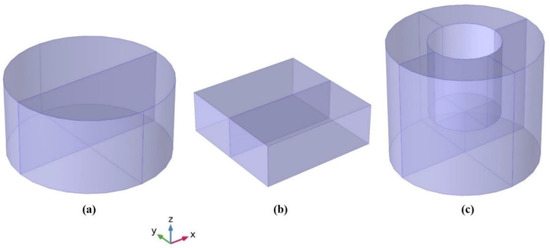
Figure 2.
Composite samples used for drying experiment: (a) cylindrical, (b) rectangular, (c) hollow cylinder with closed end.
4. Results and Discussion
This section presents the heating and drying modeling results and experimental comparison to validate the model. Baseline input parameters for heating and drying are shown in Section 2.1. Initially, simulations were carried out using two waveguide dimensions and compared with the experimental results to build the credibility on the waveguide cross-sectional dimensions. Subsequently, a comprehensive description of the influence of electromagnetic fields and microwave power absorption on heating is presented. This is followed by drying characteristics of different foam samples based on the modeling and experimental results. Parameters such as microwave power, sample size and time-increment affecting the drying behavior are also discussed.
4.1. Effect of Waveguide Dimensions
The microwave oven system used for experiments includes a rectangular waveguide through which the microwaves operate in TE10 mode at a frequency. Dimensions of the waveguide are a rough estimation depending on the microwave size. Moreover, the microwave manual lacked the information related to the waveguide size. Therefore, in this study, two waveguides were employed to develop confidence in the approximate size of the waveguide. It should be noted that energy cannot propagate in the TE10 mode if the frequency is lower than the cut-off frequency that can be determined from Equation (7), see Section 2.1. Equation (7) includes two parameters a and b which correspond to the depth and height of the waveguide. Microwave heating results of a water sample with and for two waveguides are listed in Table 5. Two waveguide dimensions and were considered. Waveguide dimensions are selected based on the microwave excitation frequency of 2.45 GHz propagating at TE10 mode. The calculated times for heating for the waveguide of showed close proximity to experimental results.
Table 5.
Calculated times (seconds) of heating for rectangular waveguides and comparison with experimental data.
4.2. Comparison of Modeling and Experimental Results for Heating
The heating models consider the cylindrical water sample at two power levels, and , with varying volume and microwave power. Figure 3 depicts the calculated time from the modeling of two power levels to attain a temperature of 100 °C. Calculated and measured data points are depicted with cross and circle markers for 30% power input. It can be seen that the calculated heating time is slightly higher than the measured time. For instance, heating 100 of water at 30% power measured approximately 174 s whereas from the model 187 s was calculated. This minor discrepancy can be attributed to the loss of the electromagnetic waves to the materials available in the microwave cavity. Besides that, rotational turntable instigating uniform heating lowered the heating time experimentally. On the contrary, non-uniform heating due to stationary turntable increased the heating time in the simulation. The average errors between the calculated and measured heating times for 30% and 70% power inputs were 9% and 13%, respectively. Liu et al. [34] developed a microwave heating simulation on food samples and showed the variations in temperature distributions for stationary and rotating turntable. Temperature of the stationary cylindrical sample increased more quickly in some specific locations, but the interior part remained low compared to the rotational sample. Higher power significantly reduced the time to reach 100 °C. For example, the measured heating time for a volume of water at was 174 s but at the elapsed time was 69 s. Overall, lowered the heating time by almost 60% compared with for water samples.
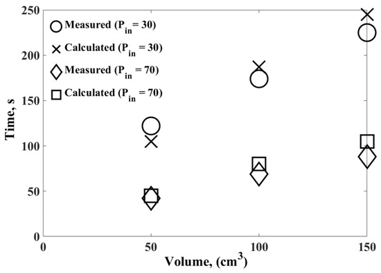
Figure 3.
Comparison of the calculated and measured results for heating 100 of water to 100 °C at 30 and 70% power levels.
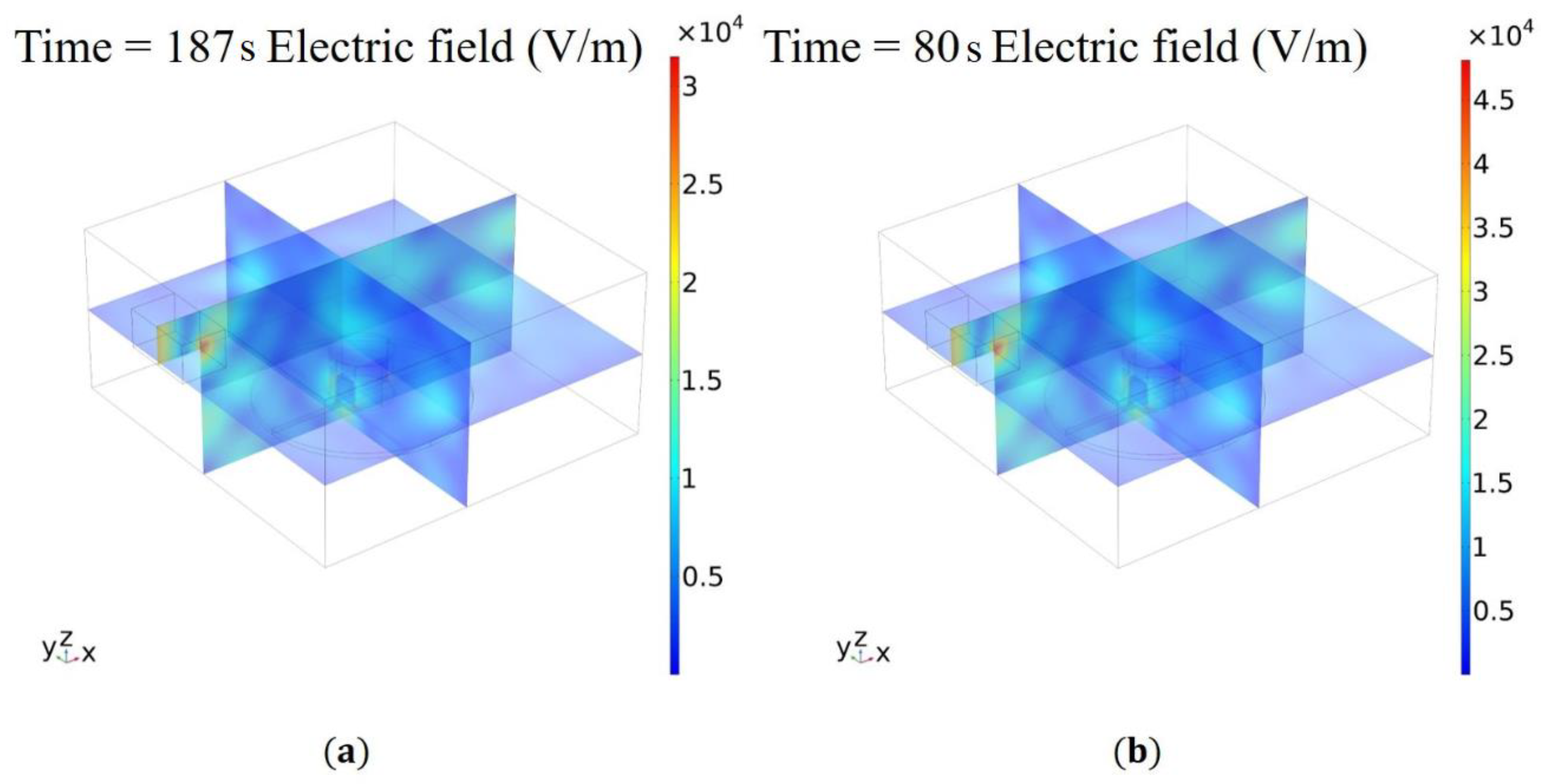
Hypothetical temperature distributions of the water sample obtained from modeling at two microwave power levels and are depicted in Figure 4a,b. Irradiation in microwave created hot and cold spot regions due to the high and low energy regions. This is caused by the superimposition of electromagnetic waves that bounced back and forth inside the oven cavity rendering a shape of resonating electric field with high and low electric field. Since modeling was carried out on stationary turntable and the water was not allowed to flow by convection, the generated heat elevated temperature quickly in the hot spot regions. It can be seen that the maximum predicted temperature generated at the bottom surface for 30% and 70% microwave power levels were and , respectively; the average temperature was, however, . These high temperatures would never exist in the real case since they are above the boiling point of water. In reality, there may be localized vapor generation that dissipates the energy and causes some flow within the volume. Figure 4 exhibits the cold spot regions remained at 320 and after microwave heating. The temperature distribution patterns indicate that the locations of cold and hot spots regions are the same for both cases. This behavior is expected because the modeling was carried out on a solid domain without any flow possible to even out hot and cold regions. Even with the model neglecting the flow and vaporization of water, it still has potential to predict drying and heating by using average temperatures.
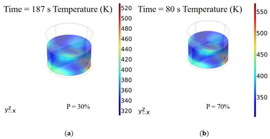
Figure 4.
Comparison of the calculated and measured results for heating 100 of water to 100 °C at 30% (a) and 70% (b) power levels.
Microwave power strongly influenced the heat generation in water sample because higher power input causes more microwave absorption. To investigate the effect of microwave power, modeling was carried out on of water with a variation of power levels of 10, 30, 50, 70, 90 and 100%. The larger absorption of microwave energy by the water sample at high power levels increased the temperature within the material. Non-uniform distribution of temperature throughout the sample is dominated by the microwave power, but the average temperature is calculated to find the heating rate. Figure 5 shows the time for heating of at various power input to reach . The predicted time at different power levels matches the experimental results within experimental error except for the 10% power case. This deviation is probably caused by heat loss of water samples experimentally that was not accounted for in the modeling. For long heating times, this loss could be significant and could explain the low predicted value in Figure 5.
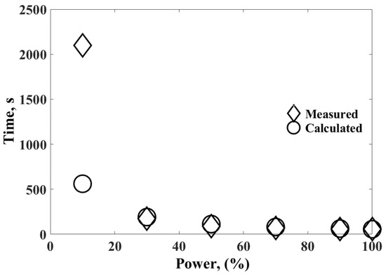
Figure 5.
Effect of microwave power on time to reach the temperature of 100 °C for a water sample of .
Heat generation in a sample varies with respect to the distribution of the electric field. Electromagnetic waves are reflected by the waveguides and cavity walls forms high and low energy regions in the microwave. As shown in Figure 6, the electric field for at power level ranged between to whereas at power it induced a range between .

Figure 6.
Electric field generated in the microwave chamber during the heating experiment of a water sample of at 30% (a) and 70% (b) power levels.
4.3. Comparison of Modeling and Experimental Results for Composite Drying
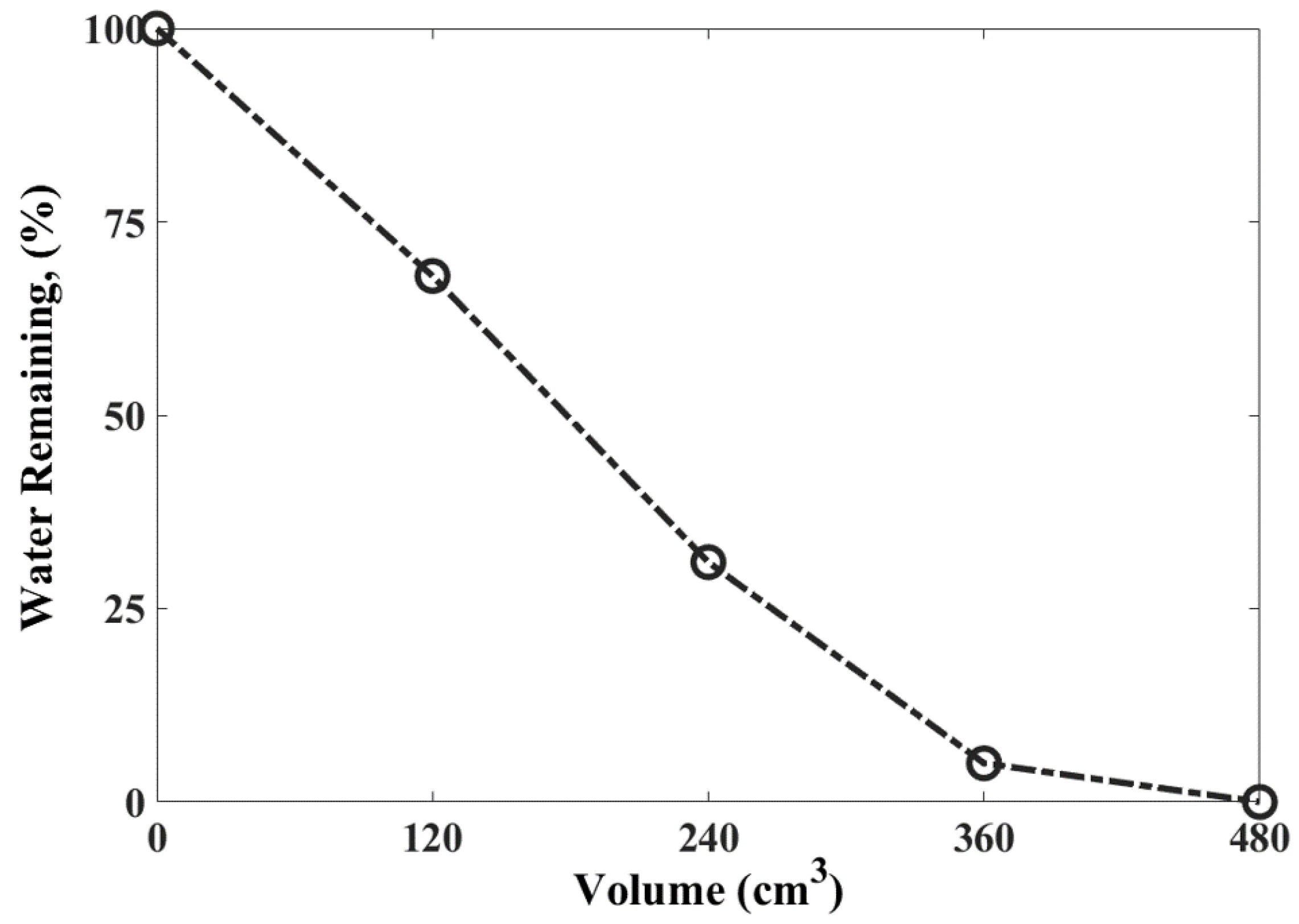
The experimental validation of modeling for foams with varying size and shape is presented. During experiments, the moisture loss due to evaporation of water reduced the weight of the samples. This phenomenon is imitated in the drying simulation by reducing the volume determined from Equation (12). Drying scenarios presented in Table 3 are considered to establish this modeling approach as a viable method. Figure 7 shows the moisture loss for the drying modeling case I of irradiated at 100% power level. The height and radius of the cylinder are 3.1 and 3.2 cm, respectively. Time-increment of 120 s was employed. At the early stage of drying, evaporation rate was quicker due to high energy generation. A gradual reduction in the evaporation rate and low energy was observed as the volume decreased. Without considering the mass transfer physics, the model is quite robust to predict moisture loss. This drying simulation technique implemented on three samples namely cylindrical, rectangular and HCCE presenting strong influence of the microwave power, sample size and time steps are discussed in the following sections.

Figure 7.
Calculated results for the implementation of stepwise drying simulation technique on 100 of water at 1200 W power.
Microwave drying predictions do not strongly depend on the time-increment used between applying Equation (12) to reset the sample temperature. In the model, the average temperature is allowed to go above the boiling point of water, but at the end of the increment, the energy gained is used to calculate the water mass loss, and the temperature of the sample is reset to 100 °C. The effect of time-increment on the rectangular sample at microwave power is shown in Figure 8 using three different time-increments. The calculated moisture loss using 120 s time-increment is in good agreement with the experimental results. The other time-increments have some deviation near the end of drying. These deviations are likely from the sample mostly being dry, but the increment time has not subtracted water from the sample at those points. The 480 s time-increment resulted in a deviation in the moisture loss prediction likely because the reduction of water content does not reflect the real case. However, the agreement of the model for the smaller time increments with the experiments are within 10%. While this modeling technique neglects the motion of water from the sample and allows water temperature to hypothetically go above the boiling point of water, the key prediction of drying time as a function of process and material parameters is good.
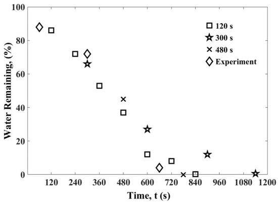
Figure 8.
Comparison of effect of time-steps for a rectangular composite sample being dried at . Total sample weight = 45 g.
To further validate the model, comparison of the calculated and measured water loss of cylindrical sample with 30 and 70% power for a time-increment of 120 s is depicted in Figure 9: the model agrees with the experimental measurements within 10%. The amount of water decreases with time as expected. Measured data points were recorded at higher intervals than calculated points. The calculated time to dry the sample to 10% water content at 30% power was 1200 s while drying at 70% power reduced the required time to 720 s. The incremental method to remove water from the sample seems to agree well with the experimental results.
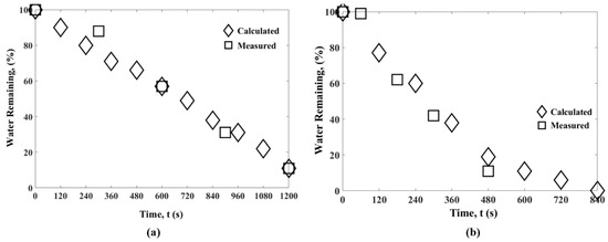
Figure 9.
Comparison of the moisture loss of cylindrical foam with a dried at and .
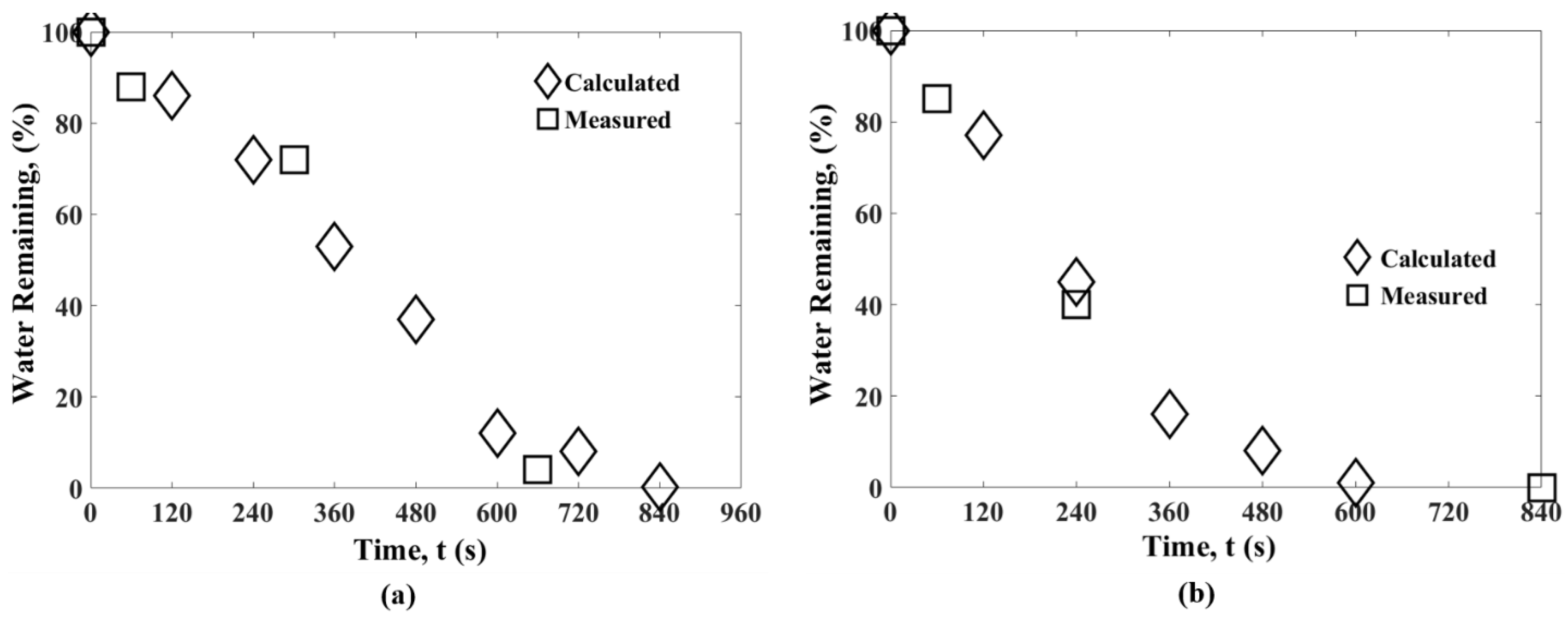
The evolution of moisture loss for the rectangular sample that includes CNF and TMP fibers with a volume of at power levels of and is illustrated in Figure 10. Calculated results showed strong agreement with the measured data points. It is evident from the calculated results that the evaporated water in each time-increment was consistent until the sample reached a moisture content less than 15%. This behavior can be characterized by the slightly flattened region of the plummeting trend at the end. Analysis of the results imply that drying prediction is accurate with the variation of drying time for the influence of power. Analysis of the results imply that drying prediction is accurate for the variation of power on the rectangular sample. It is important to note that the calculated time to dry the sample at was 840 s which is lower than the time elapsed at (600 s). It means that reduced the drying time by 21%. Measured values showed a similar behavior.
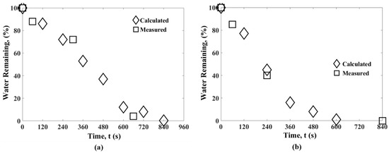
Figure 10.
Comparison of the moisture loss of rectangular foam sample with a at (a) and (b).
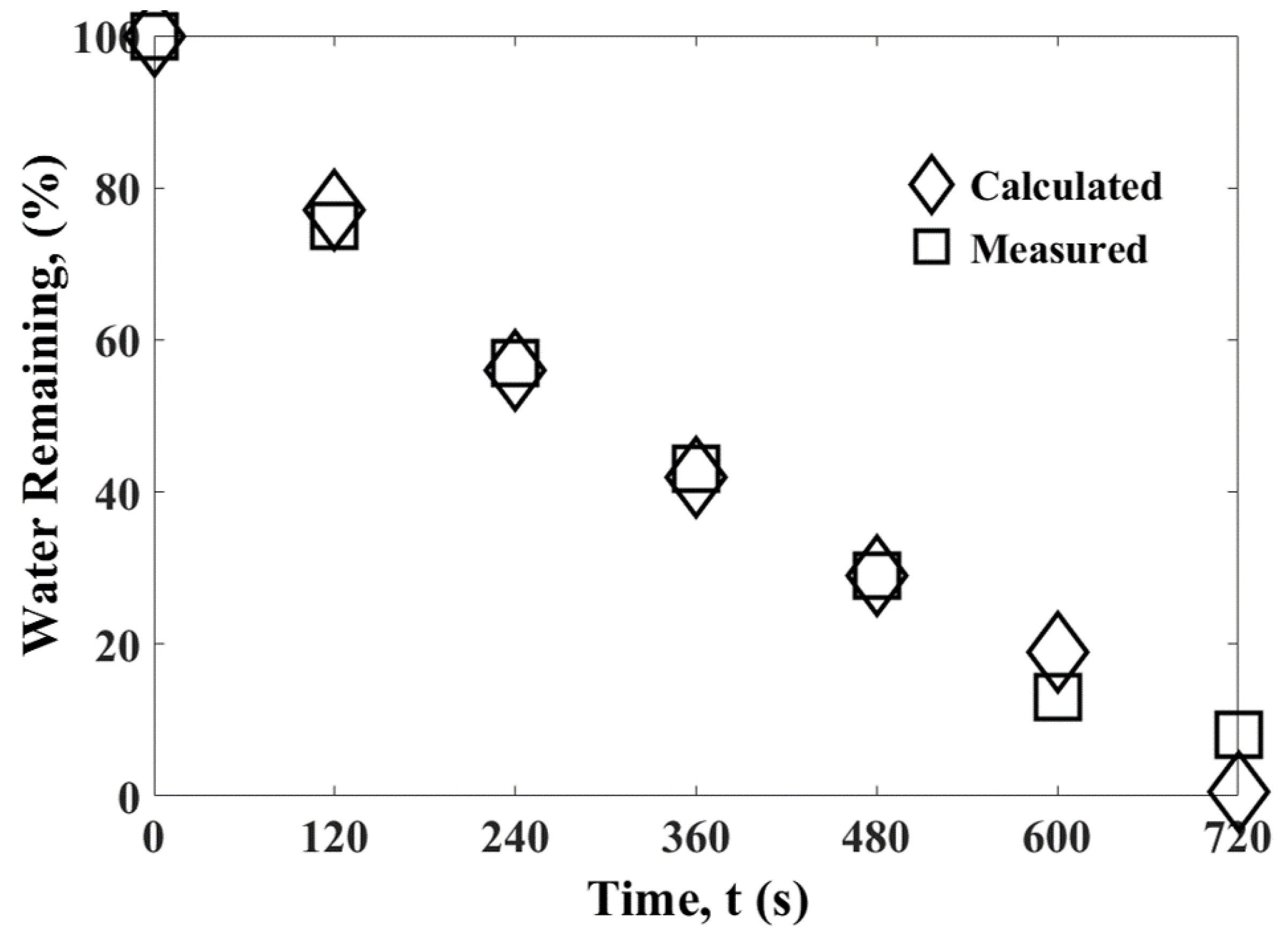
Microwave drying modeling was implemented on a hollow cylindrical sample with a closed end at . The evolution of moisture loss for this sample is shown in Figure 11. Experimental data points were recorded at every 2 min time intervals consistent with the simulation time-increment. It is important to note that the hollow cylinder with closed end (HCCE) sample had a relatively complex shape and the quantification of the moisture loss using the same time-step in experiments and modeling provided more confidence in the drying simulation technique. The calculated and measured data points for HCCE sample, as shown in Figure 11, are in strong agreement. Total time elapsed to fully dry the sample was 720 s.

Figure 11.
Evolution of moisture loss for hollow cylindrical closed end foam at .
The effects of the sample size on moisture loss during microwave drying were studied based on the calculated time predicted following the modeling approach explained earlier. With the increment of the size of the sample, drying time is expected to be longer. In order to investigate the effects of the sample size on drying, two cylindrical foam samples with a volume of and were studied. The samples are the same in radius with the variation of height. Figure 12 shows the calculated drying time for the two cylindrical samples. Elapsed time to fully dry the 500 sample was 1200 s, much higher than that for the 100 sample. However, the available data points show the amount of water loss for the two samples shows a slight deviation. Although both samples were irradiated at the same power level, the evaporated mass was different. With the higher volume, even though the evaporated mass was higher, the associated energy due to the microwave absorption was relatively lower.
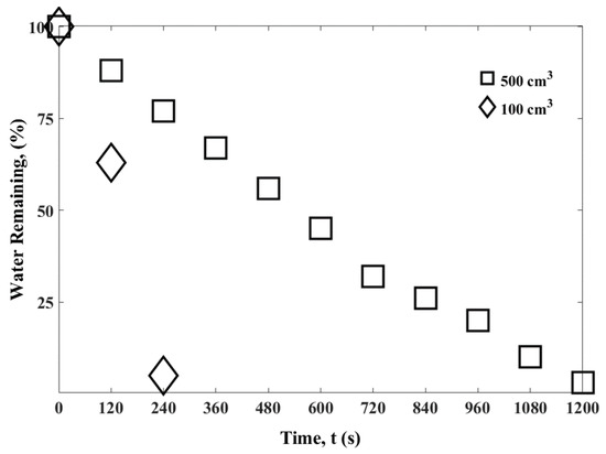
Figure 12.
Water loss of foams as a function of drying time and sample size at .
As discussed, the predictions on the microwave drying from models compared well with the experimental values for the variation of power, sample geometry and sample size for the range of parameters studied. This indicates that the simple time-increment method picks up the key physics of the situation and is able to help predict the drying time of these samples based on various material and operating parameters. There is not a need to account for mass transfer inside the sample or outside the sample and fluid motion. These assumptions and the time-increment method greatly reduce the complexity of the situation.
5. Modeling and Experimental Limitations
Microwave radiation and heating is a complex phenomenon that requires integration of multiple physics to produce viable solutions. A simplified model that assumes different characteristics can still accurately predict the heating and drying times. The modeling approach adopted in this study is based on the following assumptions: (1) turntable rotation on heating and drying modeling was disregarded, (2) microwave heating was performed on the solid domain to estimate time for water boiling, and (3) CNF and TMP fibers are treated as a single entity when microwave drying the lignocelluloisic foam. Drying through porous structures poses more challenges as it requires to determine mass transfer using Darcy’s law and (4) microwave drying modeling assumes that the entire sample undergoing microwave irradiation is water, not a porous structure. A major contribution of this study is the development of a microwave drying framework for predicting drying times of lignocellulosic foam materials. Modeling and experimental results were compared, and both offered reasonable estimates of drying time. Experimental limitations are: (1) Microwave power and geometry is one of the major limitations. Due to limited size and maximum 1200 W power, it was not possible to conduct an experiment on the huge volume of water. Hence, Figure 12 only includes modeling results, (2) it was not possible to measure the weight of the sample continuously so that increment size is large in the measured values, and (3) another limitation could be the rotation of the glass plate where we have no control. A stationary glass plate may have improved the slight error between the experimental and measured values.
6. Conclusions
This study focused on developing a modeling approach to predict the microwave drying for porous foam structures made from wood fibers and CNF. A 3D-FE coupled electromagnetic and heat transfer analysis was developed for microwave heating of water for varying volumes under different power inputs. Correct estimation of the waveguide size led to accurate prediction of heating time of water for varying volumes presenting temperature distributions of high and low energy regions for an average temperature of 100 °C. Variation of microwave input power for a constant volume of water also demonstrated good agreement with experiments. Water evaporation was implemented in the FE model by equating energy absorption to the mass loss due to evaporation over a fixed time-increment. Microwave drying predictions were compared to experimental results for cylindrical, rectangular and HCCE samples for varying power inputs and sample sizes for 120 s time increment. This modeling technique showed strong agreement of drying predictions with the experimental results. Cylindrical foams revealed that moisture loss and energy absorption substantially depend on the sample size. Overall, this novel concept FE modeling approach can be used to predict microwave drying time for porous foam structures as well as save time and reduce cost to manufacture the materials industrially.
Author Contributions
Conceptualization, M.T. (Mohammad Tauhiduzzaman), I.H., D.B. and M.T. (Mehdi Tajvidi); methodology, M.T. (Mohammad Tauhiduzzaman), I.H., D.B. and M.T. (Mehdi Tajvidi); validation, M.T. (Mohammad Tauhiduzzaman) and I.H.; formal analysis, M.T. (Mohammad Tauhiduzzaman) and I.H.; investigation, M.T. (Mohammad Tauhiduzzaman) and I.H.; resources, D.B. and M.T. (Mehdi Tajvidi); writing—original draft preparation, M.T. (Mohammad Tauhiduzzaman); writing—review and editing, M.T. (Mohammad Tauhiduzzaman), I.H., D.B. and M.T. (Mehdi Tajvidi); supervision, M.T. (Mehdi Tajvidi); project administration, M.T. (Mehdi Tajvidi); funding acquisition, M.T. (Mehdi Tajvidi). All authors have read and agreed to the published version of the manuscript.
Funding
This project was funded by USDA/ARS Cooperative Agreement Number 58-0204-0-100 awarded to the University of Maine. This project was also supported by the USDA National Institute of Food and Agriculture, McIntire-Stennis. Project #042120. Maine Agricultural and Forest Experiment Station Publication Number 3861.
Institutional Review Board Statement
Not applicable.
Informed Consent Statement
Not applicable.
Data Availability Statement
I choose to exclude this statement.
Acknowledgments
The authors thank the above-mentioned funding agencies for the financial support of this research.
Conflicts of Interest
The authors declare no conflict of interest.
References
- Wicklein, B.; Kocjan, A.; Salazar-Alvarez, G.; Carosio, F.; Camino, G.; Antonietti, M.; Bergström, L. Thermally insulating and fire-retardant lightweight anisotropic foams based on nanocellulose and graphene oxide. Nat. Nanotechnol. 2015, 10, 277–283. [Google Scholar] [CrossRef] [PubMed]
- Lavoine, N.; Guillard, V.; Desloges, I.; Gontard, N.; Bras, J. Active bio-based food-packaging: Diffusion and release of active substances through and from cellulose nanofiber coating toward food-packaging design. Carbohydr. Polym. 2016, 149, 40–50. [Google Scholar] [CrossRef] [PubMed]
- Hamedi, M.; Karabulut, E.; Marais, A.; Herland, A.; Nyström, G. Nanocellulose aerogels functionalized by rapid layer-by-layer assembly for high charge storage and beyond. Angew. Chem.Int. Ed. 2013, 125, 12260–12264. [Google Scholar] [CrossRef]
- Martoïa, F.; Cochereau, T.; Dumont, P.J.J.; Orgéas, L.; Terrien, M.; Belgacem, M.N. Cellulose nanofibril foams: Links between ice-templating conditions, microstructures and mechanical properties. Mater. Des. 2016, 104, 376–391. [Google Scholar] [CrossRef]
- Hossen, M.R.; Talbot, M.W.; Kennard, R.; Bousfield, D.W.; Mason, M.D. A comparative study of methods for porosity determination of cellulose based porous materials. Cellulose 2020, 27, 6849–6860. [Google Scholar] [CrossRef]
- Ding, W.; Jahani, D.; Chang, E.; Alemdar, A.; Park, C.B.; Sain, M. Development of PLA/cellulosic fiber composite foams using injection molding: Crystallization and foaming behaviors. Compos. Part A Appl. Sci. Manuf. 2016, 83, 130–139. [Google Scholar] [CrossRef]
- Lavoine, N.; Bergström, L. Nanocellulose-based foams and aerogels: Processing, properties, and applications. J. Mater. Chem. A 2017, 5, 16105–16117. [Google Scholar] [CrossRef] [Green Version]
- Nechyporchuk, O.; Belgacem, M.N.; Bras, J. Production of cellulose nanofibrils: A review of recent advances. Ind. Crop. Prod. 2016, 93, 2–25. [Google Scholar] [CrossRef]
- Yousefi Shivyari, N.; Tajvidi, M.; Bousfield, D.W.; Gardner, D.J. Production and Characterization of Laminates of Paper and Cellulose Nanofibrils. ACS Appl. Mater. Interfaces 2016, 8, 25520–25528. [Google Scholar] [CrossRef]
- Amini, E.; Tajvidi, M.; Gardner, D.J.; Bousfield, D.W. Utilization of cellulose nanofibrils as a binder for particleboard manufacture. BioResources 2017, 12, 4093–4110. [Google Scholar] [CrossRef] [Green Version]
- Diop, C.I.K.; Tajvidi, M.; Bilodeau, M.A.; Bousfield, D.W.; Hunt, J.F. Evaluation of the incorporation of lignocellulose nanofibrils as sustainable adhesive replacement in medium density fiberboards. Ind. Crops Prod. 2017, 109, 27–36. [Google Scholar] [CrossRef]
- Hafez, I.; Tajvidi, M. Laminated wallboard panels made with cellulose nanofibrils as a binder: Production and properties. Materials 2020, 13, 1303. [Google Scholar] [CrossRef] [PubMed] [Green Version]
- Yildirim, N.; Shaler, S.M.; Gardner, D.J.; Rice, R.; Bousfield, D.W. Cellulose nanofibril (CNF) reinforced starch insulating foams. Cellulose 2014, 21, 4337–4347. [Google Scholar] [CrossRef]
- Dash, R.; Li, Y.; Ragauskas, A.J. Cellulose nanowhisker foams by freeze casting. Carbohydr. Polym. 2012, 88, 789–792. [Google Scholar] [CrossRef]
- Svagan, A.J.; Jensen, P.; Dvinskikh, S.V.; Furó, I.; Berglund, L.A. Towards tailored hierarchical structures in cellulose nanocomposite biofoams prepared by freezing/freeze-drying. J. Mater. Chem. 2010, 20, 6646–6654. [Google Scholar] [CrossRef]
- Schiffmann, R.F. Microwave and Dielectric Drying. In Handbook of Industrial Drying; CRC Press: Boca Raton, FL, USA, 2020. [Google Scholar]
- Li, H.; Shi, S.; Lin, B.; Lu, J.; Lu, Y.; Ye, Q.; Wang, Z.; Hong, Y.; Zhu, X. A fully coupled electromagnetic, heat transfer and multiphase porous media model for microwave heating of coal. Fuel Process. Technol. 2019, 189, 49–61. [Google Scholar] [CrossRef]
- Pitchai, K.; Chen, J.; Birla, S.; Gonzalez, R.; Jones, D.; Subbiah, J. A microwave heat transfer model for a rotating multi-component meal in a domestic oven: Development and validation. J. Food Eng. 2014, 128, 60–71. [Google Scholar] [CrossRef]
- Irannajad, M.; Mehdilo, A.; Salmani Nuri, O. Influence of microwave irradiation on ilmenite flotation behavior in the presence of different gangue minerals. Sep. Purif. Technol. 2014, 132, 401–412. [Google Scholar] [CrossRef]
- Rattanadecho, P. The simulation of microwave heating of wood using a rectangular wave guide: Influence of frequency and sample size. Chem. Eng. Sci. 2006, 61, 4798–4881. [Google Scholar] [CrossRef]
- Tauhiduzzaman, M.; Carlsson, L.A. Finite element modeling of face/core interface fracture in homogenized honeycomb core sandwich SCB specimens. J. Sandw. Struct. Mater. 2020, 23, 1099636219896859. [Google Scholar] [CrossRef]
- Reddy, J.N.; Gartling, D.K. The Finite Element Method in Heat Transfer and Fluid Dynamics, 3rd ed.; CRC Press: Boca Raton, FL, USA, 2010; ISBN 9781439882573. [Google Scholar]
- Feng, H.; Tang, J.; Cavalieri, R.P.; Plumb, O.A. Heat and mass transport in microwave drying of porous materials in a spouted bed. AIChE J. 2001, 47, 1499–1512. [Google Scholar] [CrossRef]
- Gulati, T.; Zhu, H.; Datta, A.K. Coupled electromagnetics, multiphase transport and large deformation model for microwave drying. Chem. Eng. Sci. 2016, 156, 206–228. [Google Scholar] [CrossRef] [Green Version]
- Huang, J.; Xu, G.; Hu, G.; Kizil, M.; Chen, Z. A coupled electromagnetic irradiation, heat and mass transfer model for microwave heating and its numerical simulation on coal. Fuel Process. Technol. 2018, 177, 237–245. [Google Scholar] [CrossRef]
- Salagnac, P.; Glouannec, P.; Lecharpentier, D. Numerical modeling of heat and mass transfer in porous medium during combined hot air, infrared and microwaves drying. Int. J. Heat Mass Transf. 2004, 47, 4479–4489. [Google Scholar] [CrossRef]
- He, Z.; Yan, Y.; Zhao, T.; Feng, S.; Li, X.; Zhang, L.; Zhang, Z. Heat transfer enhancement and exergy efficiency improvement of a micro combustor with internal spiral fins for thermophotovoltaic systems. Appl. Therm. Eng. 2021, 189, 116723. [Google Scholar] [CrossRef]
- Kadem, S.; Younsi, R.; Lachemet, A. Computational analysis of heat and mass transfer during microwave drying of timber. Therm. Sci. 2016. [Google Scholar] [CrossRef] [Green Version]
- Khan, M.I.H.; Welsh, Z.; Gu, Y.; Karim, M.A.; Bhandari, B. Modelling of simultaneous heat and mass transfer considering the spatial distribution of air velocity during intermittent microwave convective drying. Int. J. Heat Mass Transf. 2020, 153. [Google Scholar] [CrossRef]
- COMSOL. COMSOL Multiphysics® v.5.5a; COMSOL, Inc.: Burlington, MA, USA, 2020. [Google Scholar]
- Lin, B.; Li, H.; Chen, Z.; Zheng, C.; Hong, Y.; Wang, Z. Sensitivity analysis on the microwave heating of coal: A coupled electromagnetic and heat transfer model. Appl. Therm. Eng. 2017, 126, 949–962. [Google Scholar] [CrossRef]
- Buttress, A.; Jones, A.; Kingman, S. Microwave processing of cement and concrete materials—Towards an industrial reality? Cem. Concr. Res. 2015, 68, 112–113. [Google Scholar] [CrossRef]
- Datta, A.K. Fundamentals of Heat and Moisture Transport for Microwaveable Food Product and Process Development. In Handbook of Microwave Technology for Food Application; CRC Press: Boca Raton, FL, USA, 2020. [Google Scholar]
- Liu, S.; Fukuoka, M.; Sakai, N. A finite element model for simulating temperature distributions in rotating food during microwave heating. J. Food Eng. 2013, 115, 49–62. [Google Scholar] [CrossRef]
- Amini, E.; Hafez, I.; Tajvidi, M.; Bousfield, D.W. Cellulose and lignocellulose nanofibril suspensions and films: A comparison. Carbohydr. Polym. 2020, 250, 117011. [Google Scholar] [CrossRef] [PubMed]
- Hafez, I.; Tajvidi, M. Comprehensive Insight into Foams Made of Thermomechanical Pulp Fibers and Cellulose Nanofibrils via Microwave Radiation. ACS Sustain. Chem. Eng. 2021, 9, 10113–10122. [Google Scholar] [CrossRef]
- Amini, E.N.; Tajvidi, M.; Bousfield, D.W.; Gardner, D.J.; Shaler, S.M. Dewatering Behavior of a Wood-Cellulose Nanofibril Particulate System. Sci. Rep. 2019, 9, 14584. [Google Scholar] [CrossRef] [PubMed] [Green Version]


Publisher’s Note: MDPI stays neutral with regard to jurisdictional claims in published maps and institutional affiliations. |
© 2021 by the authors. Licensee MDPI, Basel, Switzerland. This article is an open access article distributed under the terms and conditions of the Creative Commons Attribution (CC BY) license (https://creativecommons.org/licenses/by/4.0/).