
Research of Flow Stability of Non-Newtonian Magnetorheological Fluid Flow in the Gap between Two Cylinders †


Abstract
:1. Introduction
2. Experiment, Reynolds and Taylor Number
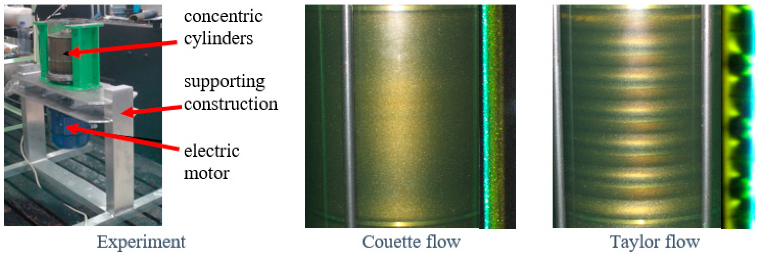
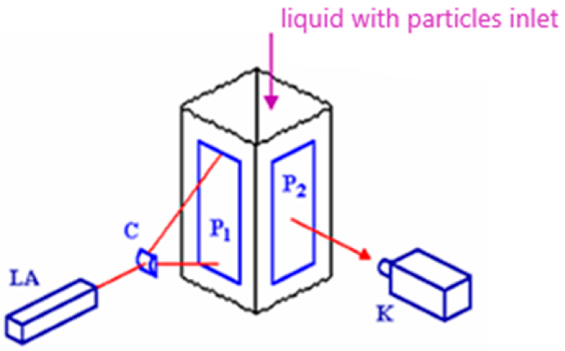
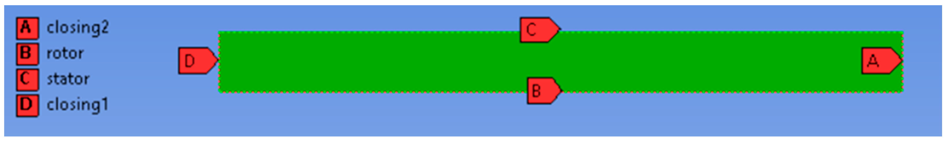
2.1. Experimental Equipment
| R1 = 65 mm | radius of the inner cylinder |
| R2 = 80 mm | radius of the outer cylinder |
| s = 15 mm | thickness of the annulus (R2 − R1) |
| L = 170 mm | length of the inner cylinder |
2.2. Physical Properties of Liquids
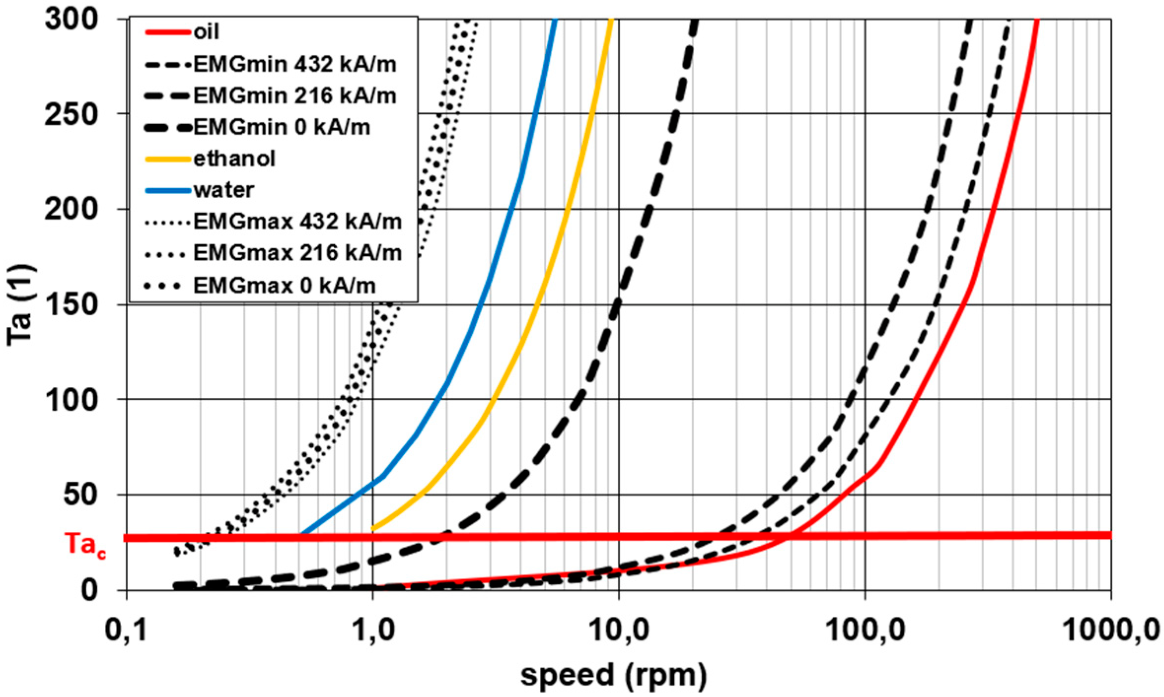
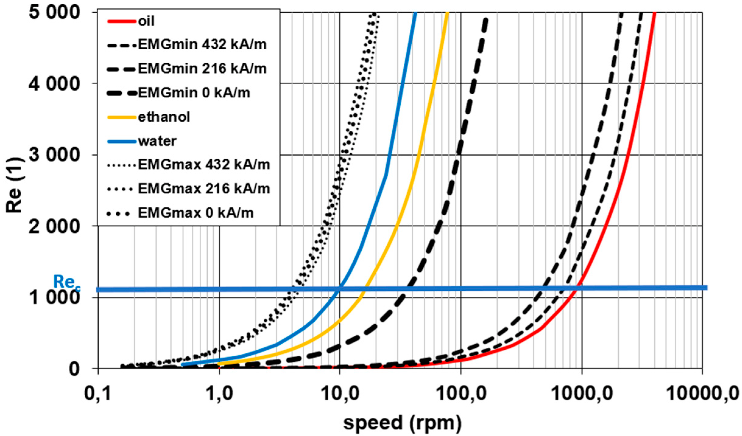
2.3. Ta, a Re Number
3. Mathematical Model
4. Experimental Results
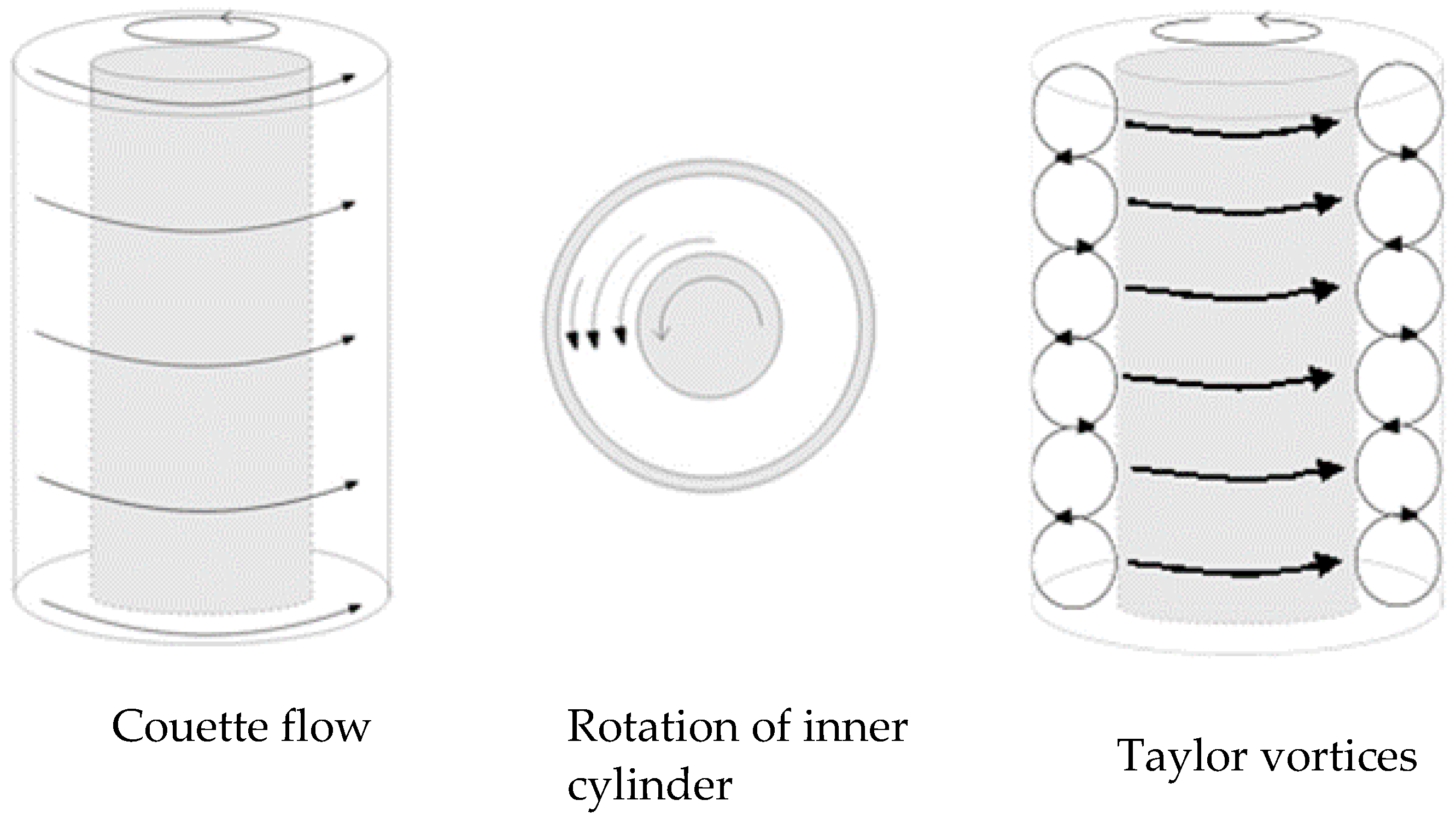
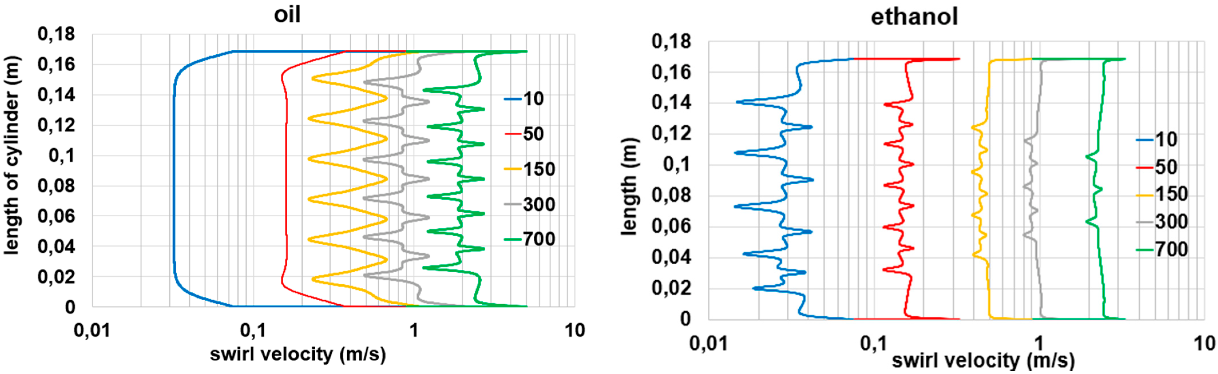
- Taylor vortices can be observed mainly in the area of laminar flow, so, in ethanol, they appear at a lower speed, while vortex structures in oil are formed at the speed of 130 rpm;
- the wave mode has not yet manifested;
- turbulence in ethanol causes vortex structures to be illegible;
- the experiment with the EMG 900 fluid was not performed. It was not possible to ensure the flow in the annulus and, at the same time, to influence it by means of a magnetic field acting perpendicular to the direction of load.
5. Numerical Simulation
5.1. Numerical Simulation—Oil, Ethanol and EMG 900
- swirl velocity in logarithmic coordinates <0.001; 5>
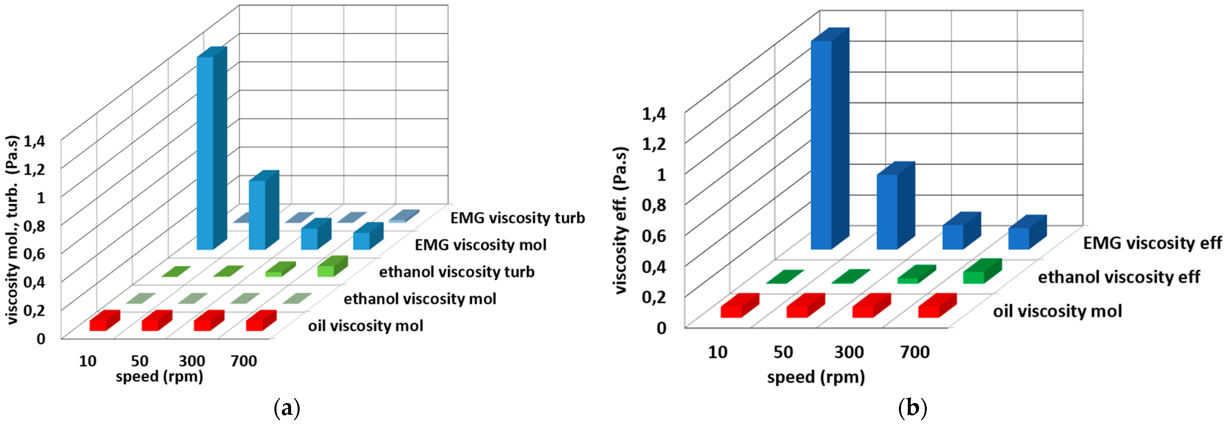
- molecular viscosity <0; 1.4>
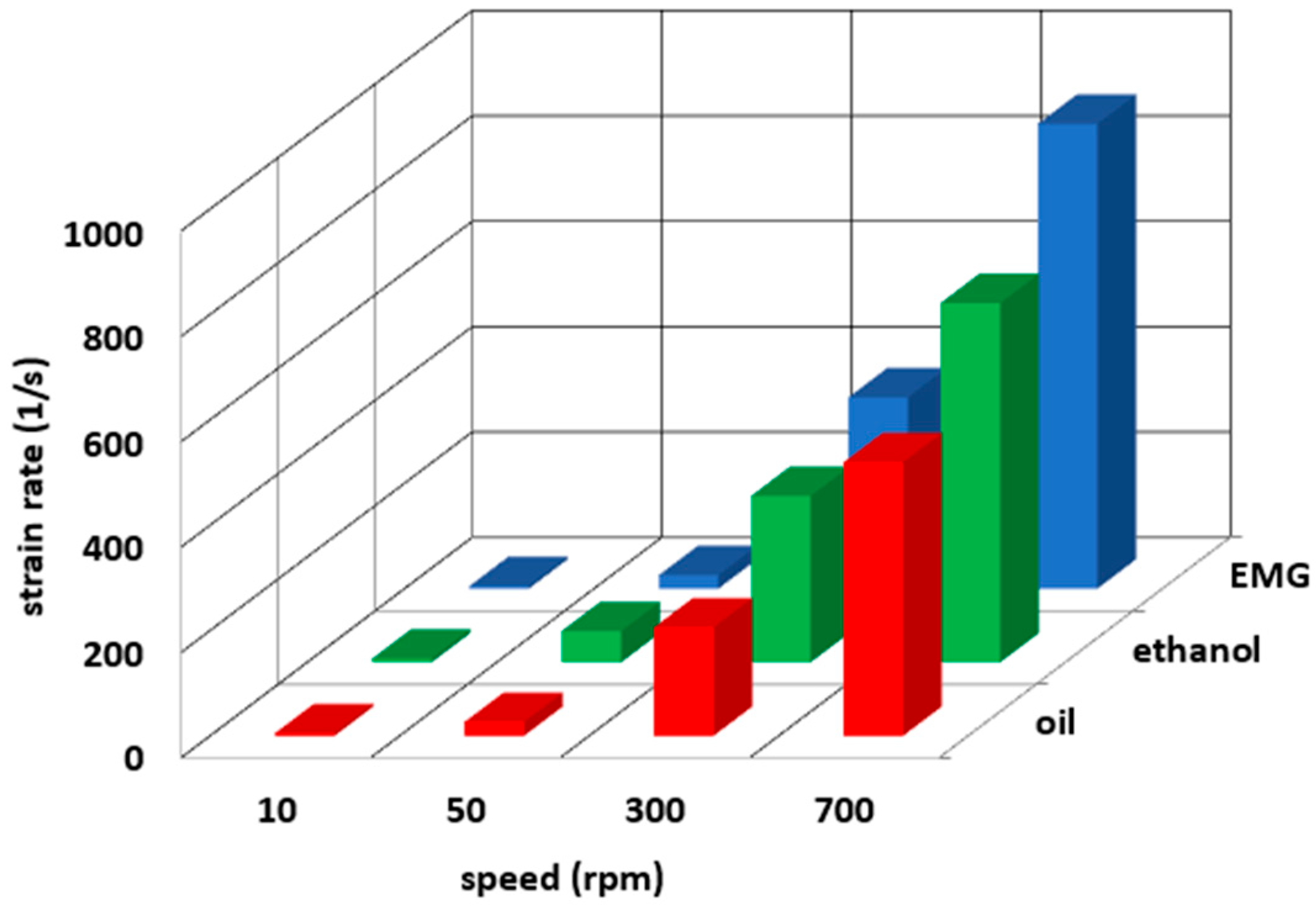
- strain rate in logarithmic coordinates <1; 100,000>
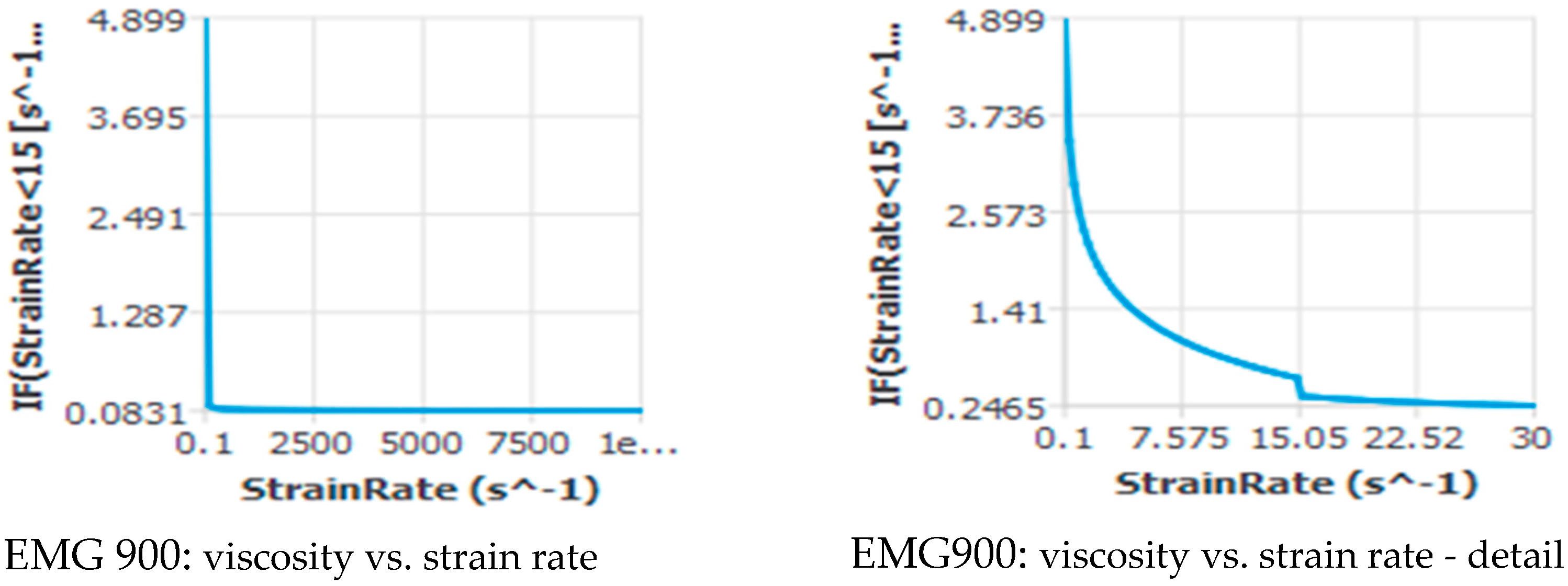
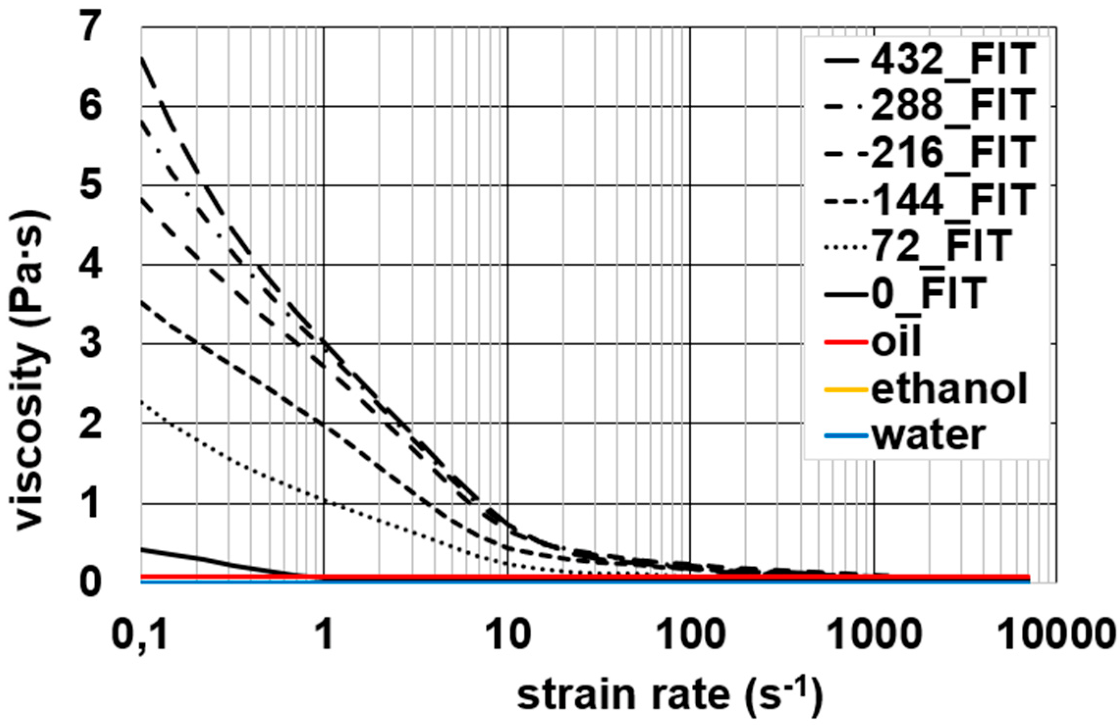
5.2. Evaluation of Viscosity of Non-Newtonian Fluid EMG 900
- laminar flow: values of the molecular viscosity and strain rate are written in black;
- turbulent flow: values of the molecular, turbulent and effective viscosities and strain rate are written in red.
6. Discussion
- single-phase flow and the formation of vortex structures (Taylor vortices) can be characterized by Taylor and Reynolds numbers;
- The mathematical model was as follows:
- −
- oil—laminar flow model;
- −
- ethanol—for speeds of 10 and 30 rpm, a model of laminar flow was used; for higher speeds, the model was turbulent.
- The flow of magnetorheological fluid was characterized by the Taylor and Reynolds numbers, depending on the shear stress, respectively, the viscosity and intensity of the magnetorheological field. An analytical evaluation of the Taylor and Reynolds numbers was difficult, so these values were determined for the minimum and maximum viscosity values at a given intensity in the magnetorheological field. For given speeds and electromagnetic field values, it was possible to estimate whether the flow was laminar or turbulent and, in addition, whether Taylor vortices would appear.
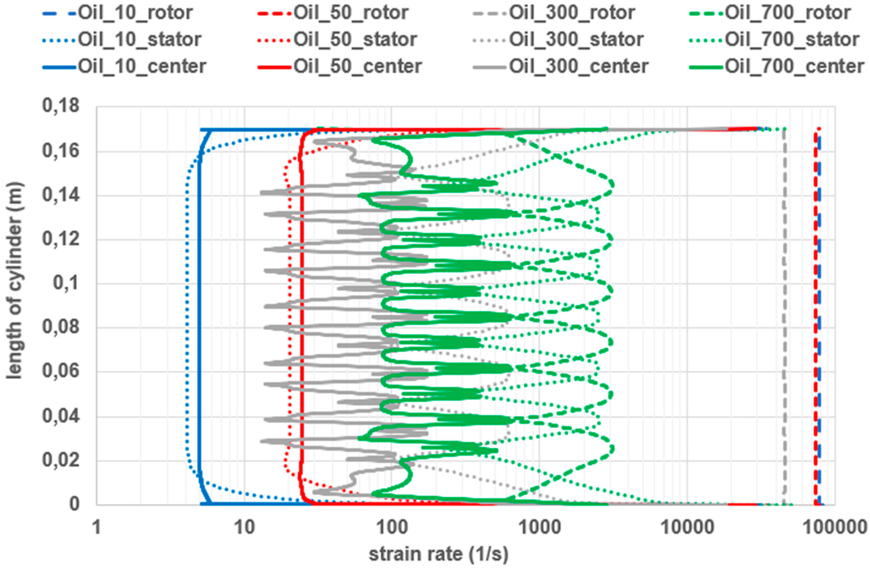
- The strain rate and viscosity were not constant within the range; the mean values of these quantities could be determined.
- The mathematical model was as follows:
- −
- EMG 900—if the speeds were 10 and 30 rpm, the mathematical model used was laminar; for higher speeds, it was turbulent.
Author Contributions
Funding
Institutional Review Board Statement
Informed Consent Statement
Data Availability Statement
Conflicts of Interest
References
- Blums, E.; Cebers, A.; Maiorov, M. Magnetic Fluids; Walter de Gruyter: Berlin, Germany; New York, NY, USA, 1997; 416p, ISBN 3-11-014390-0. DM 378. [Google Scholar]
- Odenbach, S. Ferrofluids Lecture Notes in Physics; Springer: Berlin/Heidelberg, Germany. Available online: http:/www.springer.de/phys/ (accessed on 26 November 2002).
- Fialová, S.; Kozubková, M.; Jablonská, J.; Havlásek, M.; Pochylý, F.; Šedivý, D. Journal bearing with non-Newtonian fluid in the area of Taylor vortices. IOP Conf. Ser. Earth Environ. Sci. 2019, 240, 062013. [Google Scholar] [CrossRef]
- ANSYS Fluent Theory Guide; ANSYS Inc: Canonsburg, PA, USA, 2019.
- Experimental Measurement of the Viscous Reply of the Ferrofluids in Magnetic Field; Grant Agency Project: GA101/19-06666S; Internal Research Report; Grant Agency of Czech Republic: Ostrava, Czech Republic, 2020.
- Odenbach, S.; Thurrn, S. Magnetoviscous Eflects in Ferrofluids. Technical Report; Springer: Heidelberg, Germany, 2002; ISBN 354-0430687. [Google Scholar]
- Guru, B.S.; Hiziroglu, H.R. Electromagnetic Field Theory Fundamentals; Cambridge University Press: Cambridge MA, USA, 2004; ISBN 0-521-830168. [Google Scholar]
- Chari, M.V.K.; Salon, S.J. Numerical Methods in Electromagnetism; Academic Press: San Diego, CA, USA; London, UK, 2000; ISBN 0-12-615760-X. [Google Scholar]
- Jiles, D. Introduction to Magnetism and Magnetic Materials; CRC Press: New York, NY, USA, 2016. [Google Scholar]
- Lenci, A.; Chiapponi, L. An Experimental Setup to Investigate Non-Newtonian Fluid Flow in Variable Aperture Channels. Water 2020, 12, 1284. [Google Scholar] [CrossRef]
- Tong, T.A.; Yu, M.; Ozbayoglu, E.; Takach, N. Numerical simulation of non-Newtonian fluid flow in partially blocked eccentric annuli. J. Pet. Sci. Eng. 2020, 193, 107368. [Google Scholar] [CrossRef]
- Lacassagne, T.; Cagney, N.; Balabani, S. Shear-thinning mediation of elasto-inertial Taylor–Couette flow. J. Fluid Mech. 2021, 915, A91. [Google Scholar] [CrossRef]
- Kaushik, V.; Wu, S.; Jang, H.; Kang, J.; Kim, K.; Suk, J.W. Scalable Exfoliation of Bulk MoS2 to Single- and Few-Layers Using Toroidal Taylor Vortices. Nanomaterials 2018, 8, 587. [Google Scholar] [CrossRef] [PubMed] [Green Version]
- Davey, A. The growth of Taylor vortices in flow between rotating cylinders, 1962. J. Fluid Mech. 1962, 14, 336–368. [Google Scholar] [CrossRef]
- Farník, J. Investigation of the Instabilities in between Two Rotating Coaxial Cylinders. Ph.D. Thesis, VSB-TU Ostrava, Czech Republic, 2006. [Google Scholar]
- Altmeyer, S.; Do, Y.; Lai, Y.-C. Dynamics of ferrofluidic flow in the Taylor-Couette system with a small aspect ratio. Sci. Rep. 2017, 7, 40012. [Google Scholar] [CrossRef] [PubMed] [Green Version]
- Dong, S. Direct numerical simulation of turbulent Taylor–Couette flow. J. Fluid Mech. 2007, 587, 373–393. [Google Scholar] [CrossRef] [Green Version]
- Teng, H.; Liu, N.; Lu, X.; Khomami, B. Direct numerical simulation of Taylor-Couette flow subjected to a radial temperature gradient. Phys. Fluids 2015, 27, 125101. [Google Scholar] [CrossRef]
- Maksimov, F.A. Numerical Simulation of Taylor Vortex Flows Under the Periodicity Conditions. In Applied Mathematics and Computational Mechanics for Smart Applications. Smart Innovation, Systems and Technologies; Jain, L.C., Favorskaya, M.N., Nikitin, I.S., Reviznikov, D.L., Eds.; Springer: Singapore, 2021; Volume 217. [Google Scholar] [CrossRef]
- Wang, H. Experimental and Numerical Study of Taylor-Couette Flow. PhD Theses, Iowa State University, Ames, IA, USA, 2015; p. 14462. [Google Scholar] [CrossRef]
- Baek, S.I.; Ahn, J. Large Eddy Simulation of Film Cooling Involving Compound Angle Holes: Comparative Study of LES and RANS. Processes 2021, 9, 198. [Google Scholar] [CrossRef]
- Fialová, S.; Pochylý, F.; Volkov, A.V.; Ryzhenkov, A.V.; Druzhinin, A.A. The Mathematical Model Simplification Methods for Caculating Flows in the Hydraulic Turbines Flow Path. Teploenergetika 2021, 12, 1–11. (In Russian) [Google Scholar]
- Pochylý, F.; Fialová, S.; Krausová, H. Variants of Navier-Stokes Equations. In Engineering Mechanics 2012; Book of Extended Abstracts; AV CR: Prague, Czech Republic, 2012; pp. 1011–1016. ISBN 978-80-86246-40-6. [Google Scholar]
- Kozubková, M.; Jablonská, J.; Bojko, M.; Pochylý, F.; Fialová, S. Multiphase Flow in the Gap between Two Rotating Cylinders. MATEC Web Conf. 2020, 328, 02017. [Google Scholar] [CrossRef]
- Bird, R.B.; Stewart, W.E.; Lightfoot, E.N. Transport Phenomena; John Wiley & Sons: Hoboken, NJ, USA, 2002; ISBN 0-471-41077-2. [Google Scholar]
- Fialová, S.; Pochylý, F.; Malenovský, E. Numerical analysis and simulations of the magnetic field and hydrophobicity effect on the journal bearing dynamics. Proc. Inst. Mech. Eng. Part J J. Eng. Tribol. 2017, 231, 561–571. [Google Scholar] [CrossRef]
- Šedivý, D.; Ferfecki, P.; Fialová, S. Influence of Eccentricity and Angular Velocity on Force Effects on Rotor of Magnetorheological Damper. EPJ Web Conf. 2018, 180, 555–559. [Google Scholar]
- Tuma, J.; Kozubkova, M.; Pawlenka, M.; Mahdal, M.; Simek, J. Theoretical and Experimental Analysis of the Bearing Journal Motion Due to Fluid Force Caused by the Oil Film. MM Sci. J. 2018, 2018, 2466–2472. [Google Scholar] [CrossRef]


| Unit | Water | Ethanol | Oil | |
|---|---|---|---|---|
| Density | kg/m3 | 998 | 790 | 876 |
| Kinematic viscosity | m2/s | 1.002 × 10⁻⁶ | 1.5209 × 10⁻⁶ | 8.2182 × 10⁻⁵ |
| Dynamic viscosity | Pa.s | 0.001 | 0.0012 | 0.072 |
| Unit | EMG 900 | EMG 905 | |
|---|---|---|---|
| Concentration of nanoparticles | % vol. | 17.7 | 7.8 |
| Saturation magnetization | mT | 99 | 44 |
| Density | kg/m3 | 1.74∙× 103 | 1.2∙× 103 |
| Dynamic viscosity | mPa.s | 60 | 3 |
| Melting point (at pn) | °C | −94 | −94 |
| Flash point (at pn) | °C | 89 | 89 |
| Initial magnetic susceptibility | 18.6 | 3.52 |
| Speed/Liquid | Ethanol | Oil |
|---|---|---|
| 10 |  |  |
| KERRYPNX | Ethanol | Oil | EMG 900 | ||||||||
|---|---|---|---|---|---|---|---|---|---|---|---|
| Speed | Experiment | Swirl Velocity | Molecular Viscosity | Strain Rate | Experiment | Swirl Velocity | Molecular Viscosity | Strain Rate | Swirl Velocity | Molecular Viscosity | Strain Rate |
| 10 |     |     |    | ||||||||
| 50 |     |     |    | ||||||||
| 300 |     |     |    | ||||||||
| 700 |     |     |    | ||||||||
| Speed | (rpm) | 10 | 50 | 300 | 700 | |
|---|---|---|---|---|---|---|
| oil | oil viscosity mol. | (Pa.s) | 0.0726 | 0.0726 | 0.0726 | 0.0726 |
| oil viscosity turb. | (Pa.s) | _ | _ | _ | _ | |
| oil viscosity eff. | (Pa.s) | _ | _ | _ | _ | |
| oil strain rate | (s−1) | 5.27 | 26.47 | 205.99 | 519.31 | |
| ethanol | ethanol viscosity mol. | (Pa.s) | 0.00120 | 0.00120 | 0.00120 | 0.00120 |
| ethanol viscosity turb. | (Pa.s) | _ | 0.00416 | 0.03361 | 0.07512 | |
| ethanol viscosity eff. | (Pa.s) | _ | 0.00536 | 0.03481 | 0.07632 | |
| ethanol strain rate | (s−1) | 7.13 | 59.40 | 315.88 | 682.16 | |
| EMG | EMG viscosity mol. | (Pa.s) | 1.35660 | 0.48630 | 0.14999 | 0.12029 |
| EMG viscosity turb. | (Pa.s) | _ | _ | 0.00110 | 0.01843 | |
| EMG viscosity eff. | (Pa.s) | _ | _ | 0.15816 | 0.13872 | |
| EMG strain rate | (s−1) | 5.21 | 25.94 | 363.47 | 882.62 |
Publisher’s Note: MDPI stays neutral with regard to jurisdictional claims in published maps and institutional affiliations. |
© 2021 by the authors. Licensee MDPI, Basel, Switzerland. This article is an open access article distributed under the terms and conditions of the Creative Commons Attribution (CC BY) license (https://creativecommons.org/licenses/by/4.0/).
Share and Cite
Kozubková, M.; Jablonská, J.; Bojko, M.; Pochylý, F.; Fialová, S. Research of Flow Stability of Non-Newtonian Magnetorheological Fluid Flow in the Gap between Two Cylinders. Processes 2021, 9, 1832. https://doi.org/10.3390/pr9101832
Kozubková M, Jablonská J, Bojko M, Pochylý F, Fialová S. Research of Flow Stability of Non-Newtonian Magnetorheological Fluid Flow in the Gap between Two Cylinders. Processes. 2021; 9(10):1832. https://doi.org/10.3390/pr9101832
Chicago/Turabian StyleKozubková, Milada, Jana Jablonská, Marian Bojko, František Pochylý, and Simona Fialová. 2021. "Research of Flow Stability of Non-Newtonian Magnetorheological Fluid Flow in the Gap between Two Cylinders" Processes 9, no. 10: 1832. https://doi.org/10.3390/pr9101832
APA StyleKozubková, M., Jablonská, J., Bojko, M., Pochylý, F., & Fialová, S. (2021). Research of Flow Stability of Non-Newtonian Magnetorheological Fluid Flow in the Gap between Two Cylinders. Processes, 9(10), 1832. https://doi.org/10.3390/pr9101832